
\underline{\textbf{Introduction}}
In order to understand the results of a simulation and put them into a format that everybody can see we need a method that is called post-processing. Simulation data produces many types of data, and these should be understood to be able to properly manipulate, describe and present the data in a format that is obvious to the observer.
\underline{\textbf{Cell and Point Data Types}}
There are two types of Data, cell data and point data. Cell data is the ‘raw’ data produced by the solver and ParaView correctly displays this by showing each cell filed with this scalar value. Point data, however, is interpolated data based upon cell data, this allows ParaView to display a more visually pleasing gradient.
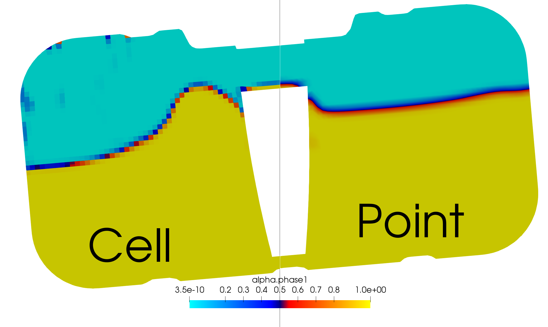
Figure 1: Visualisation shows the difference between cell and point data for scalar Phase Fraction
\underline{\textbf{Vector and Scalar Fields}}
There are two types of fields, vector and scalar. Scalar has a single value in the cell whilst vectors have 3 values for each component in the x, y and z-direction. An example of vector fields would typically be velocity in CFD or Displacement in FEA.
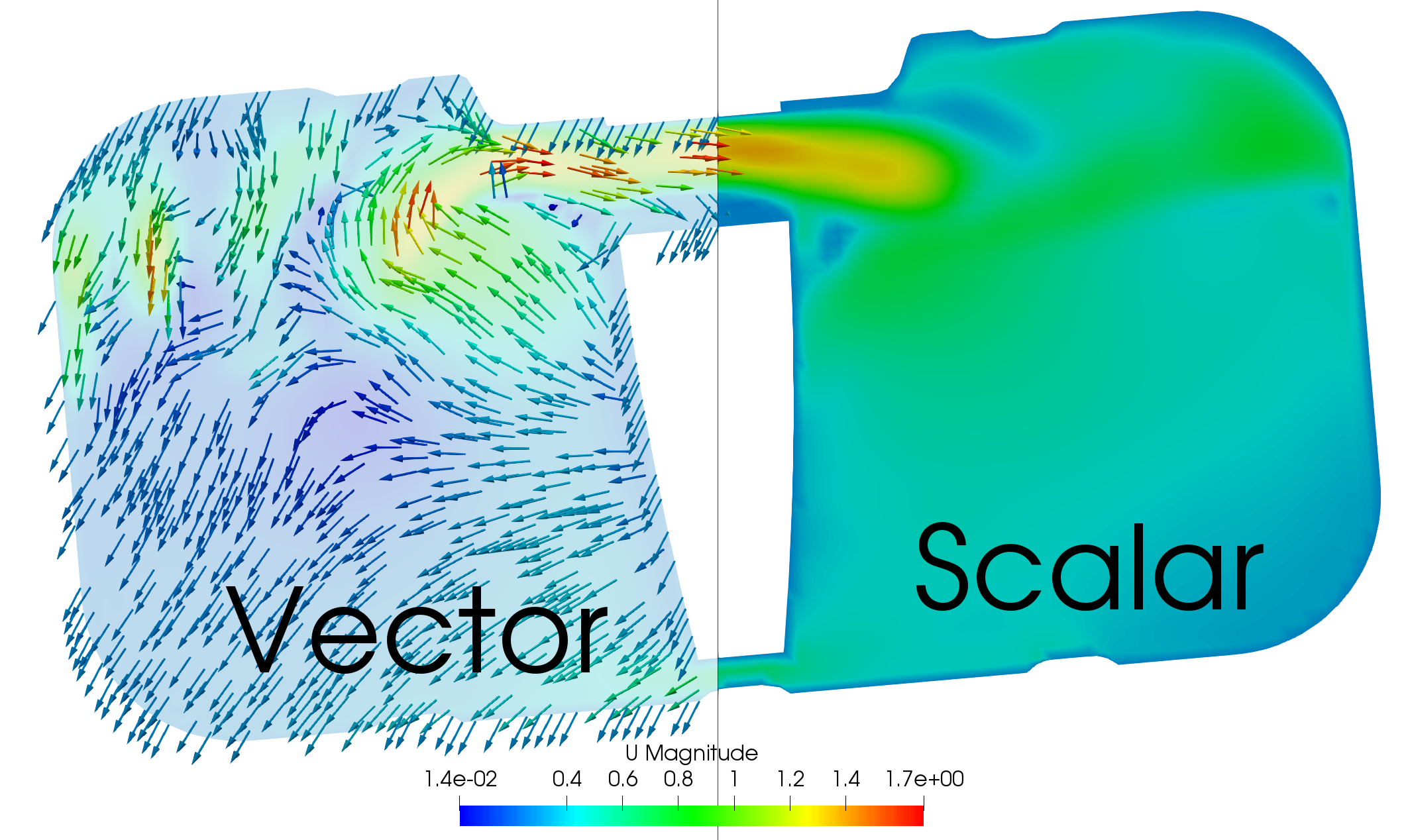
Figure 2: Velocity as a scalar (magnitude) in the cell and vector as Glyph.
ParaView will automatically display a vector type field in scalar form by magnitude if it is asked to colour by a vector, however, will use it component form if asked to display a vector type filter such as Stream Trace or Glyph.
\underline{\textbf{Field Data Manipulation}}
ParaView makes creating fields from the solver fields very easy in the form of the calculator filter, this provides methods of manipulating data to observe results in a certain way or using a unique quantity, Examples being viewing velocity in a certain plane only or creating a thermal comfort scalar respectively.
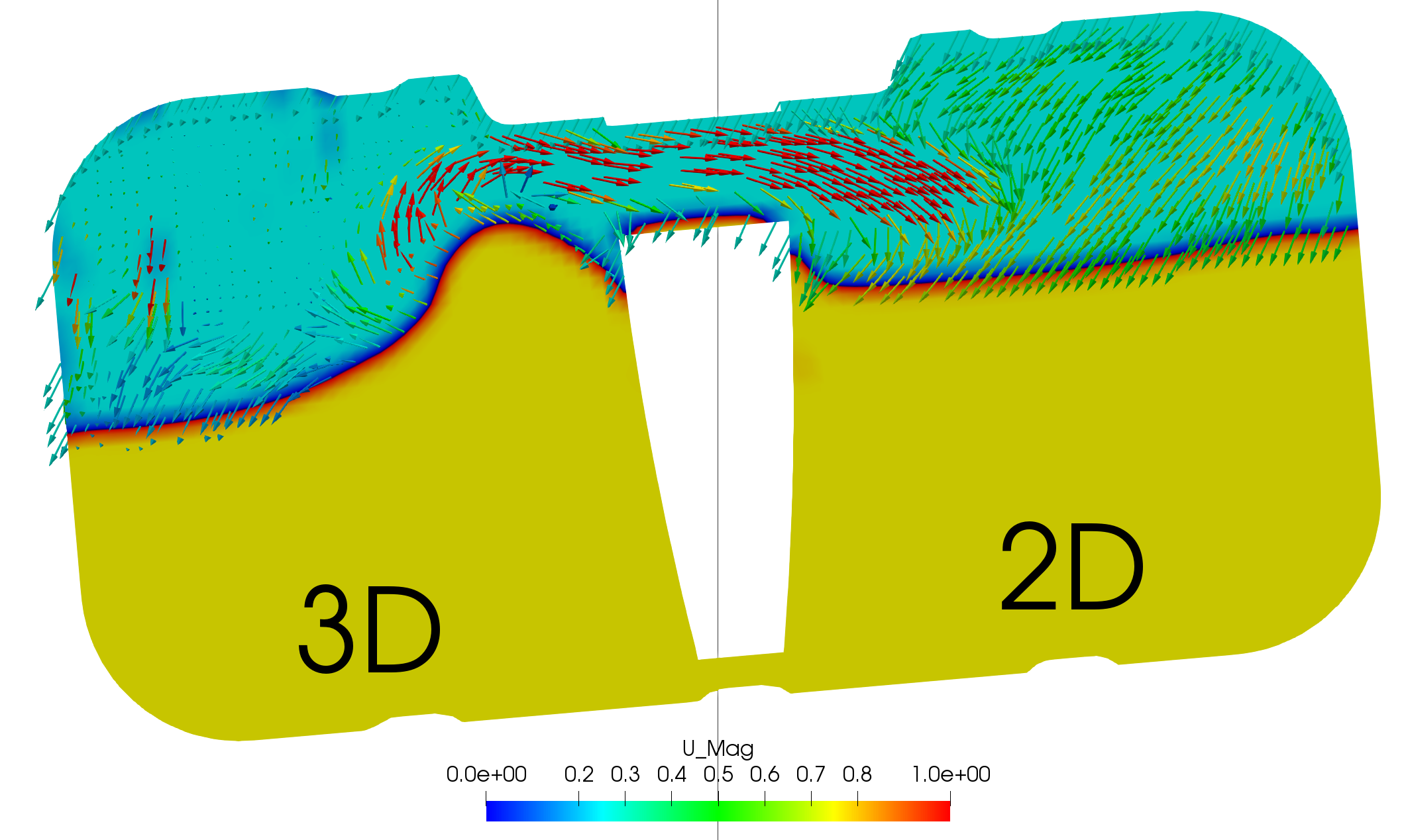
Figure 3: Velocity in 2D vs Velocity in 3D when demonstrating direction of flow on a plane
In the above Post Processing image, 3D vectors are compared to those of planar vectors, showing how much clearer planar vectors are in this example. Looking at the 3D vectors they disappear behind the slice making them only useful if they are pointing in a positive direction. The calculator was used with the formula: U_XiHat+U_ZkHat.
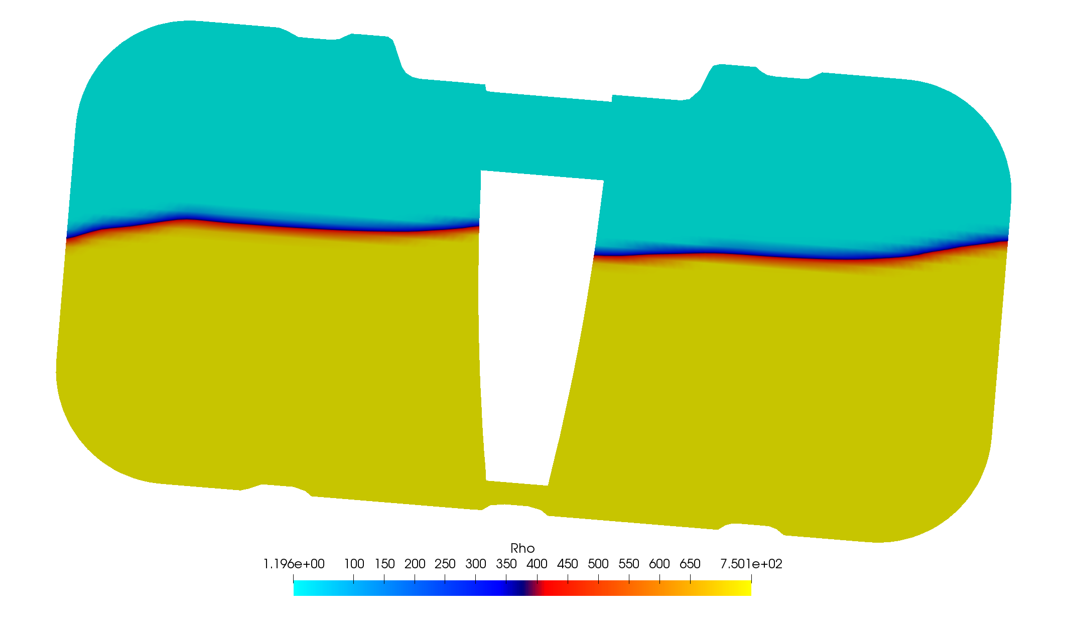
Figure 4: Demonstration of how calculator can be used to make additional scalars from raw data.
The above Post Processing image demonstrates how scalar fields can be manipulated to create new fields, the example uses phase fraction to determine density. The calculator used again with the formula: alpha.phase1 \times (750-1.1965)+1.1965, which basically uses a normalised value (phase fraction) to scale density between that of air and petrol.
\underline{\textbf{Want to read more about Post Processing in ParaView?}}
Basic filters
Layering filters (Coming soon)
Exporting your data (Coming soon)
Contributions and suggestions for improving this page are welcome, please private message @1318980