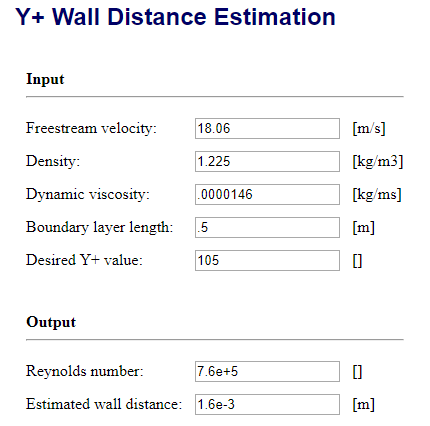
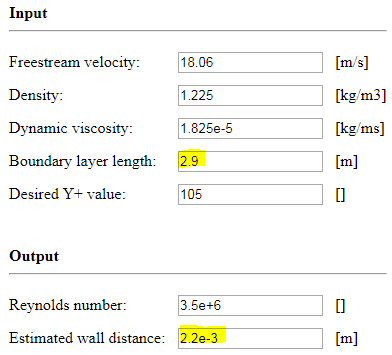
Since this is a calculator that shows centroid distance as ‘Estimated Wall Thickness’, we need to double its output of 1.6mm to get 3.2mm 1st layer thickness… That is pretty close to the 3.4mm 1st layer that got us to yPlus area average of 105
yes im up for that, the least i can do when you have helped me so much !
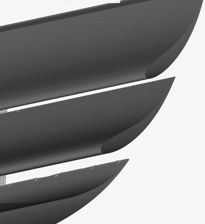
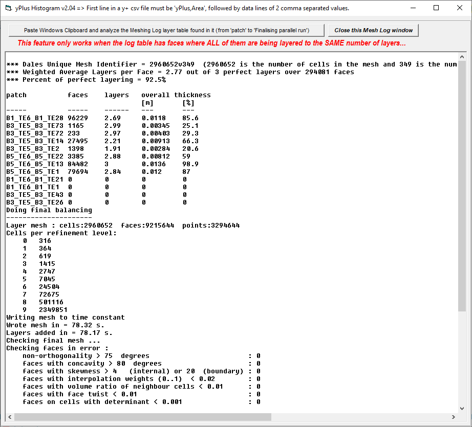
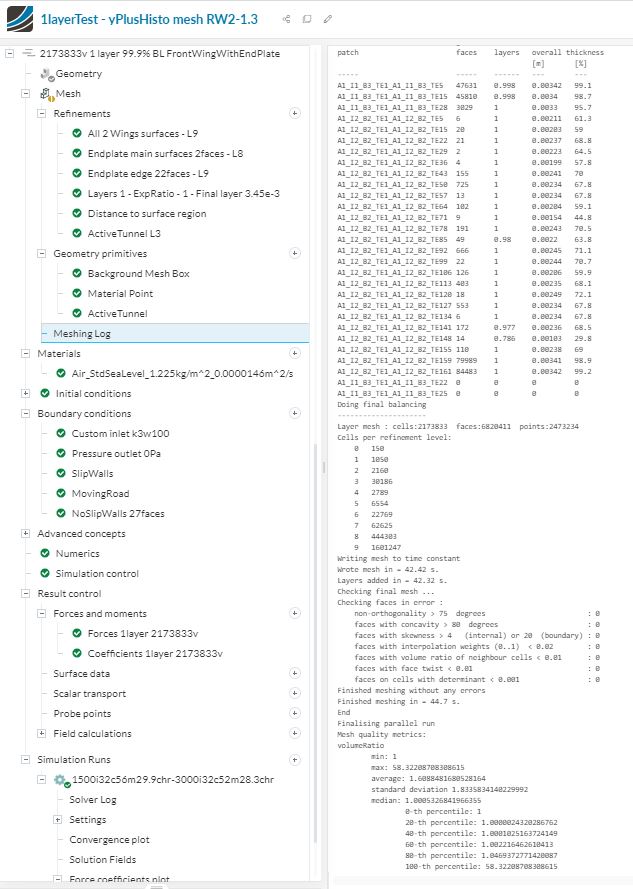
Here are the results, although i dont think this will be do - able because a half wing mesh is already at 6.6 million cells. I still have a whole car to mesh haha
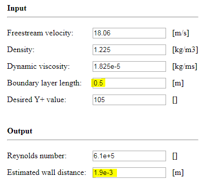
I am using different values for dynamic viscosity and boundary layer length. Any reason you are using 0.5 m for length? is it because this is the width of the rear wing? I am still using 2.9m even though its a stand alone model because eventually it will be based on the whole model length. Or do you suggest to use the actual wing sizing because there will be multiple boundary layer refinements anyways?
The Y+ changes quite a bit based on reference length
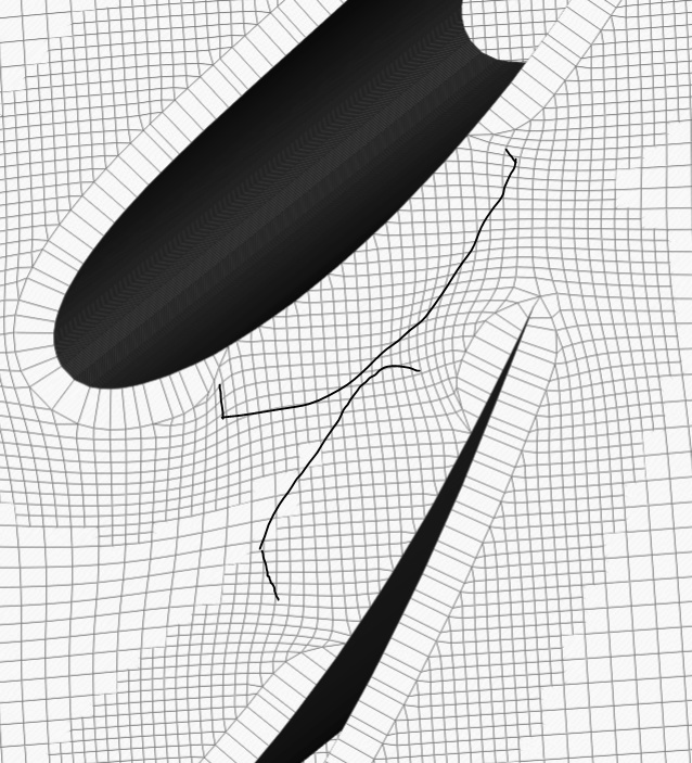
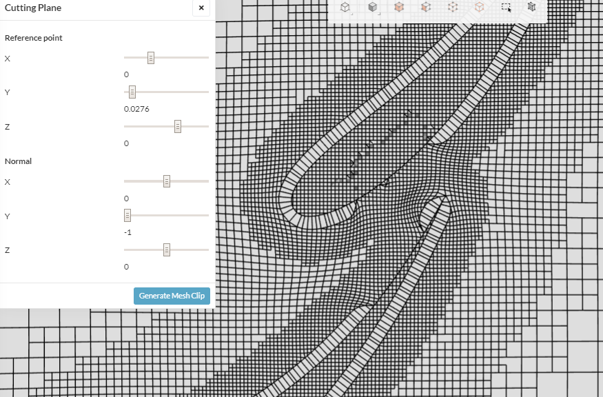
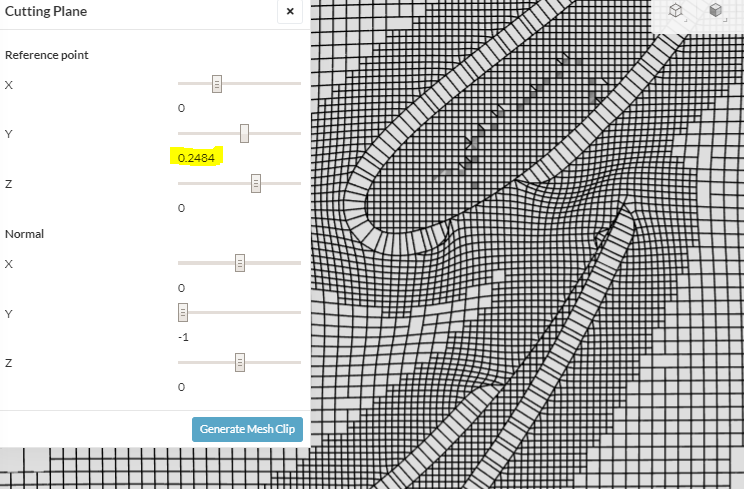
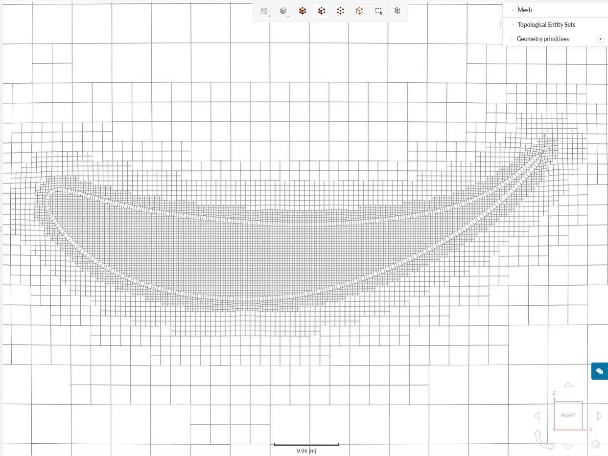
Is that at y=0, if so try meshclip at y about 0.25…
I think with some effort you can reduce that to a couple million range, you have the tools…
Yep, I still get bumps on my tire treads, I am working on that. Try feature refinement maybe. Sharp TEs are difficult sometimes. Those single cell glitches probably are not deal breakers tho…
I used the approximate length of your endplates (I think normally for cars you use length of vehicle, but here all geometry is max 0.5m, who knows what length the solvers use when they generate the yPlus values (I have not figured that out yet). I would like to assume my assumption matches what the solvers use since the results match so well…
I use the values for STD atmosphere at sea level, I have not figured where on earth the air matches the defaults in SimScale
I think it is time for a step backwards, try again with distance ref and ‘wake box high’ with no assigned faces/primitive… Perhaps set cells between levels lower too???
Once you get full coverage, then add more refinements as needed, trying to keep full coverage…
EDIT: also shouldn’t need such small cells just outside prism layer…
yea i noticed that both my wake boxes arent meshing. I originally though this was because of the lower levels in the distance to geometry refinement. Not sure. I will come back to this after i complete the sims you asked for
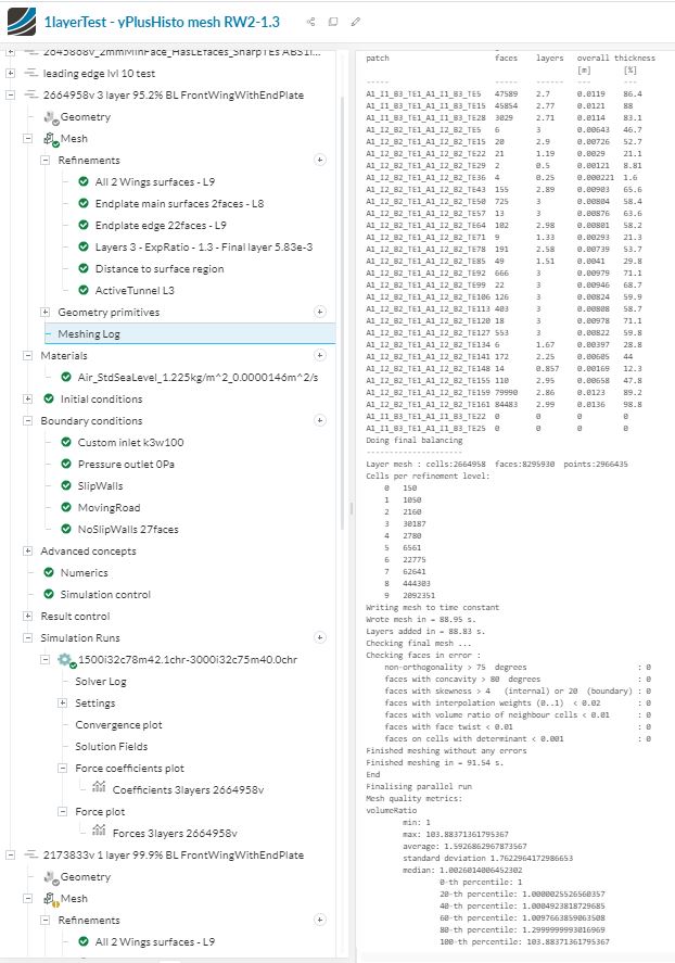
i assume your goal with this test is to compare the 3 layer BL and 1 layer BL in how well they cover Y+ surface area. I understand your concern that a 1 layer BL wont be able to measure the turbulent region that starts above the BL total thickness.
There are two main reasons for the gurney flap
described below - it moves the flow upwards increasing downforce.
2 shown in my colored lines. The red is the camber line is without gurney flap, blue is with gurney flap. It essential creates a new camber line without changing profile shape. It is used as a quick and easy way to add down force once the aero package is built
But very inefficient in terms of drag, in my opinion a better option is to modify airfoil of rear wing and get rid of that vortex drag behind the flap…
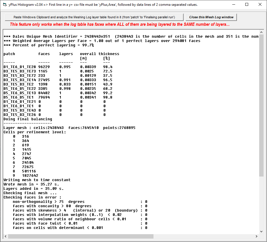
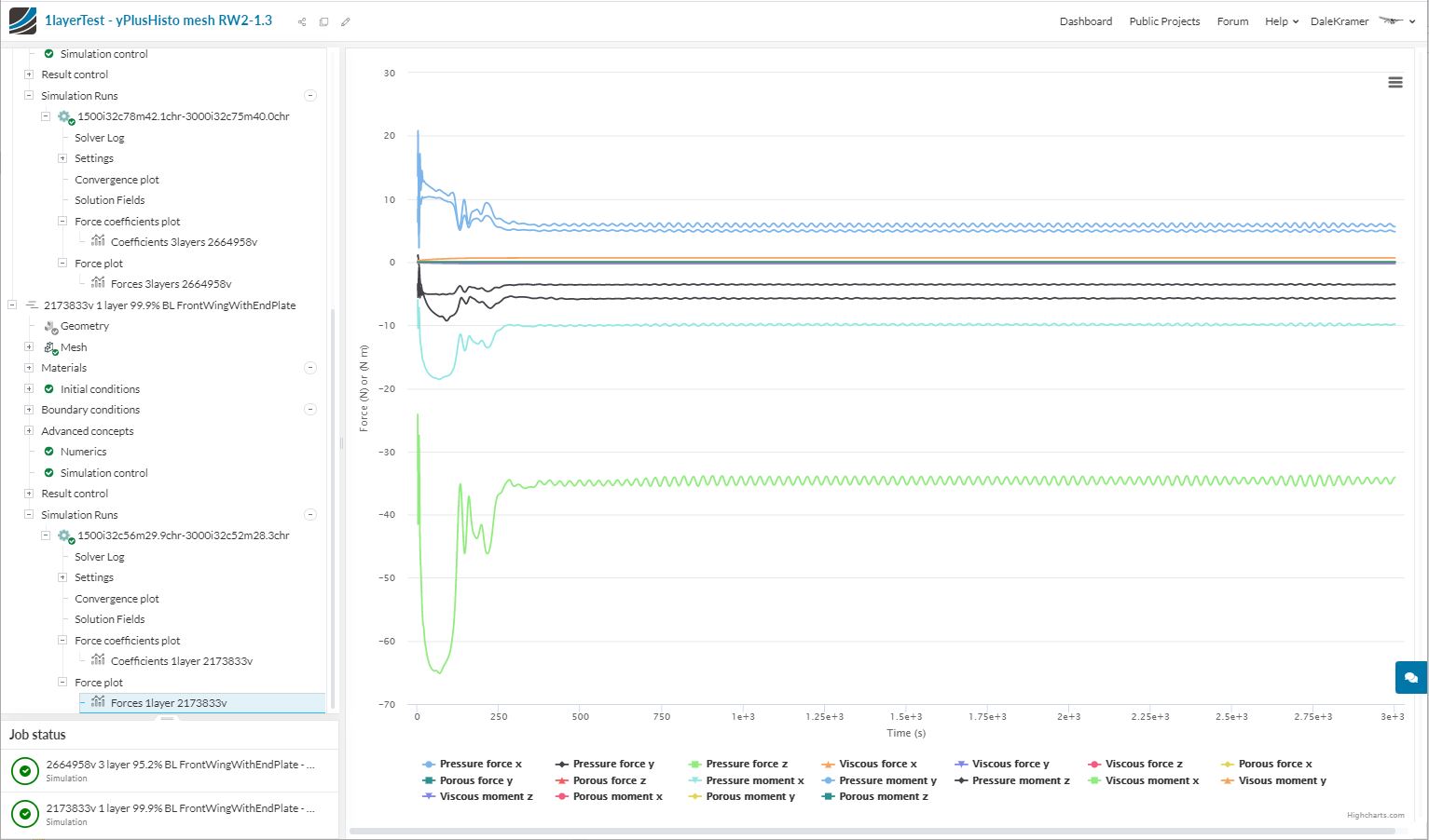
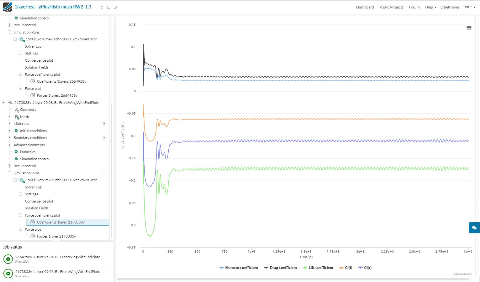
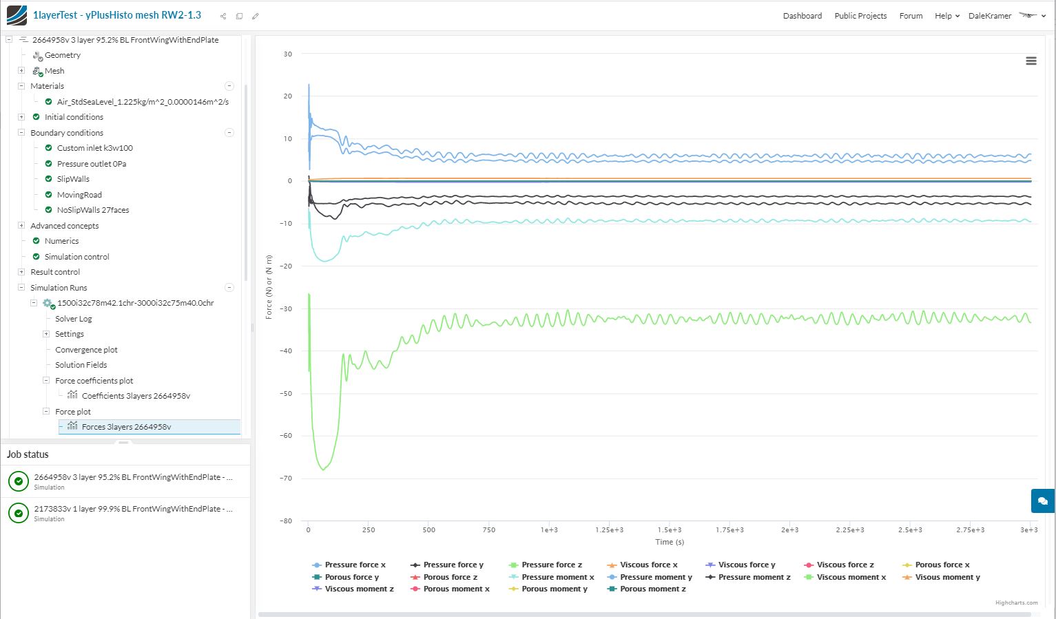
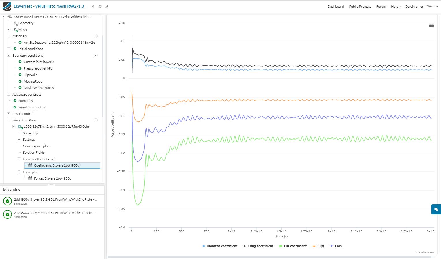
No the reason for the test is to see how much difference in pressure and viscous drag between them. If little difference the I feel fairly comfortable using 1 layer… But for the test to be valid we need same area % layered in both.
.
.
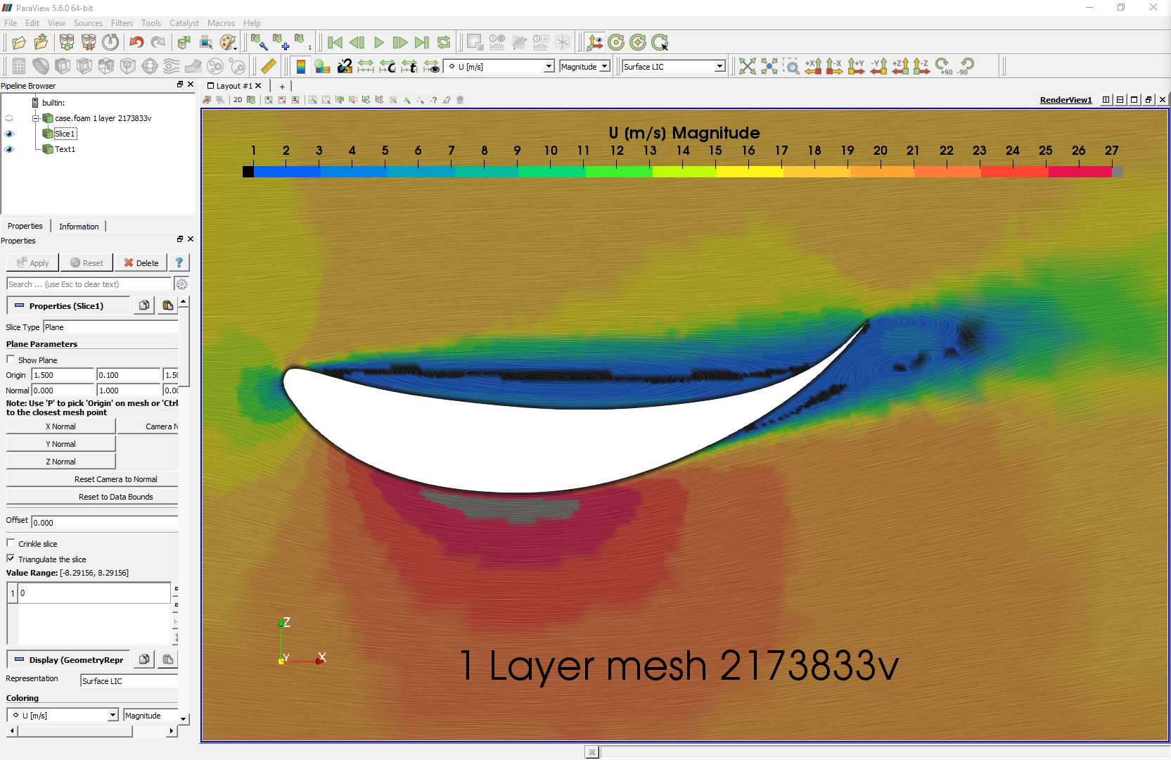
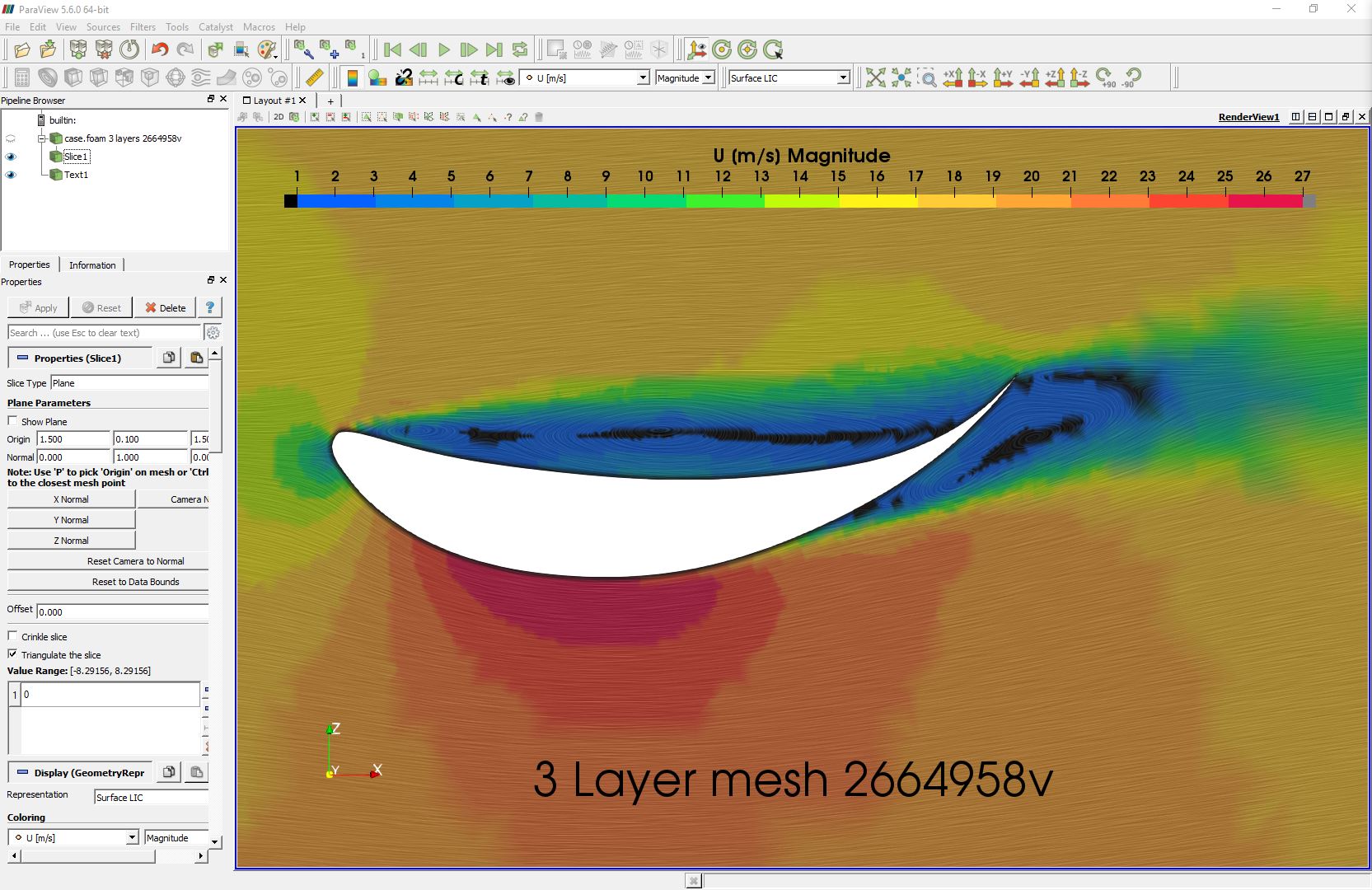
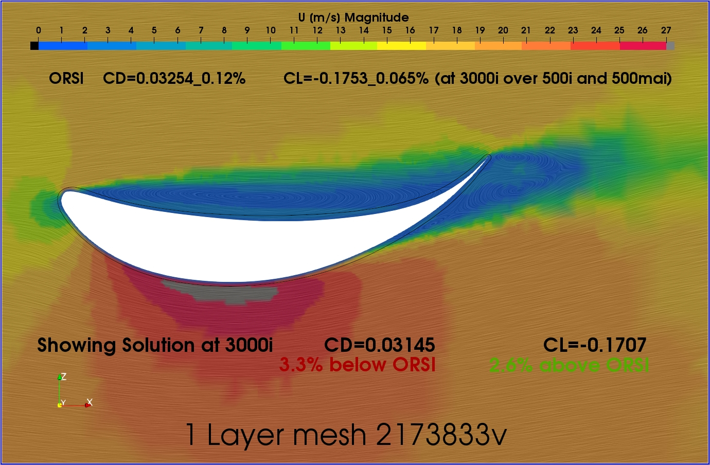
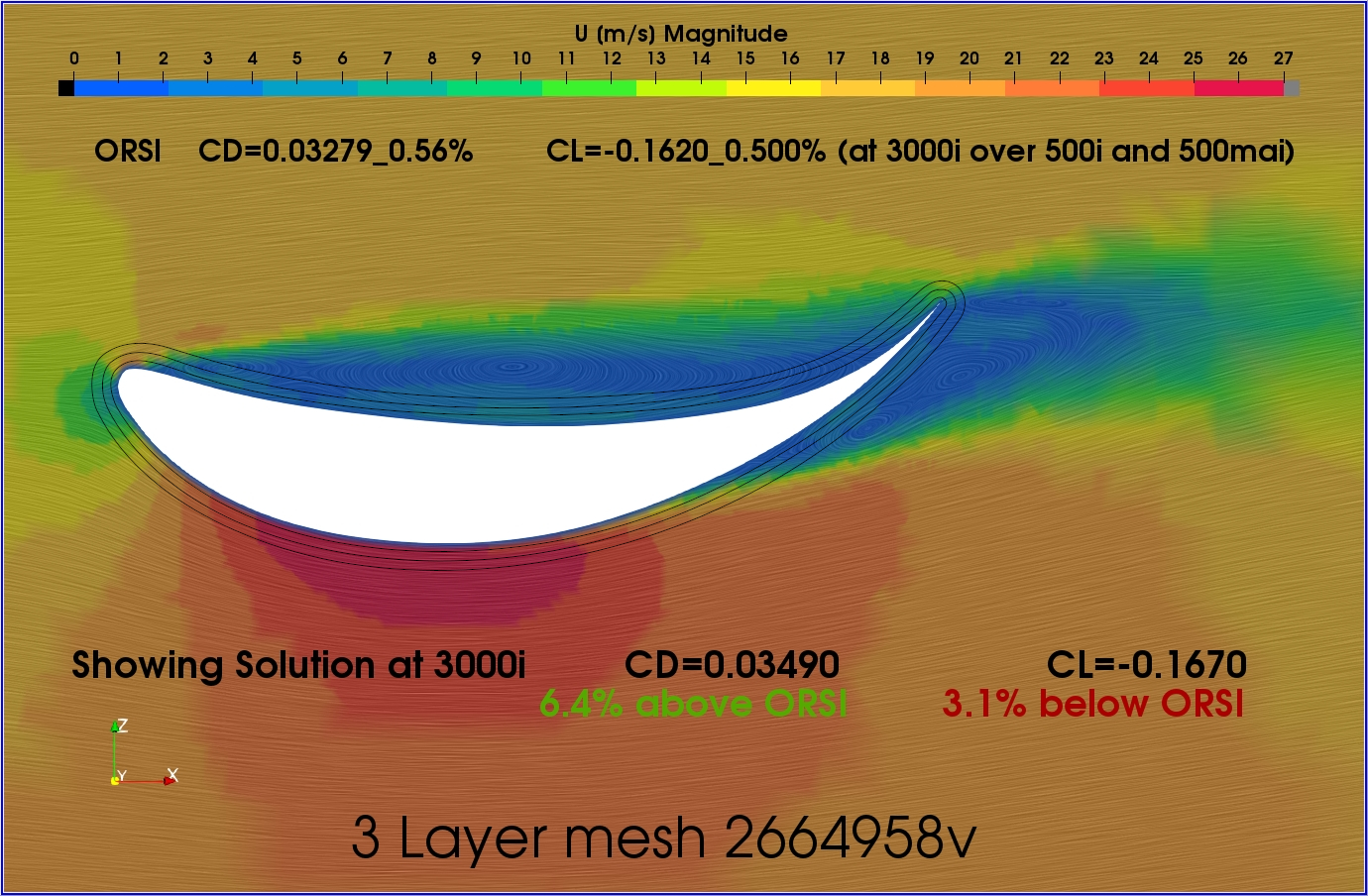
. This is really cool, you have to try it… Below are 2 images of the U magnitude ParaView plots of the results from each meshes sim run… Click on the bottom on and then use you Left and Right arrow keys to swicth between the two images… This is the only way to EASILY see the minor difference between these U magnitude plots
Congratulation Dale! Obvious winner is 1 layer mesh: you provided the proof. I discovered it (on TET mesh, when checking NACAD0012 profile on a series of endless simulations I did not want to run, but Ric, you and I, were in a kind of competition). So it does extend to HEX mesh and the proof is an elegant advance in CFD practice.
But until we can determine that ‘blindfolded best practices’ meshes and sim setups using TET cells can closely match valid experimental wind tunnel results for NACA0012 airfoil, Ahmed 3D body and Drivaer Car , I will still think that all TET CFD sims as just eye candy… (I even still have some doubts about Hex meshes )
Once again Dale you have outdone yourself. These results are extremely useful, not only for a “best practice” methodology, but also for our design report when we present the car. I think this will give us some great feedback from the judges.
The U magnitude plots look awesome! Its crazy how much of a difference this makes. I made a nifty little GIF out of your pictures too.
I think at this point I am ready to go back to the full car simulations using the 1 layer approach. Im interested to see if we can apply this BL strategy to the rest of the car. I also want to do a simulation of the car using the old method and compare the results of those. Should be interesting
Cool, but I like the arrow keys better since I can change the image at the rate I want to
.
.
.
.
.
Sooo, with much more thinking about how to use ORSI, I have come up with a realization
The ORSI moving average filter does a GREAT job at predicting a single result value of interest if the result values are oscillating about a stable value
The problem lies in the fact that simulations currently do not stop when all the results values are nearest to their current ORSI value… This means that when your simulation ends (however triggered), you could be saving the full solution set of result values at any stage of their oscillations…
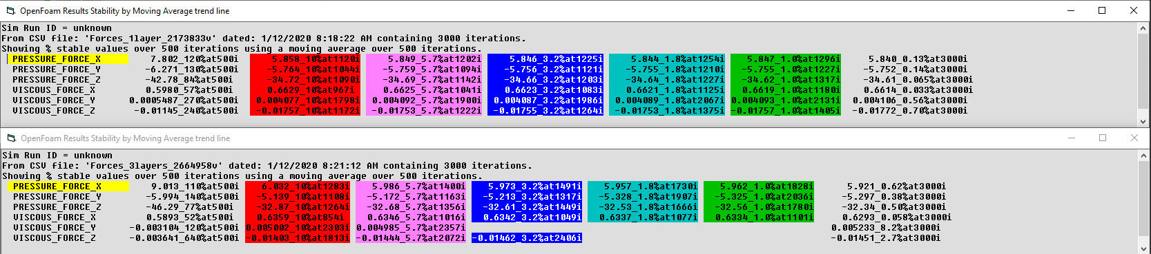
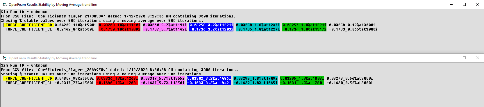
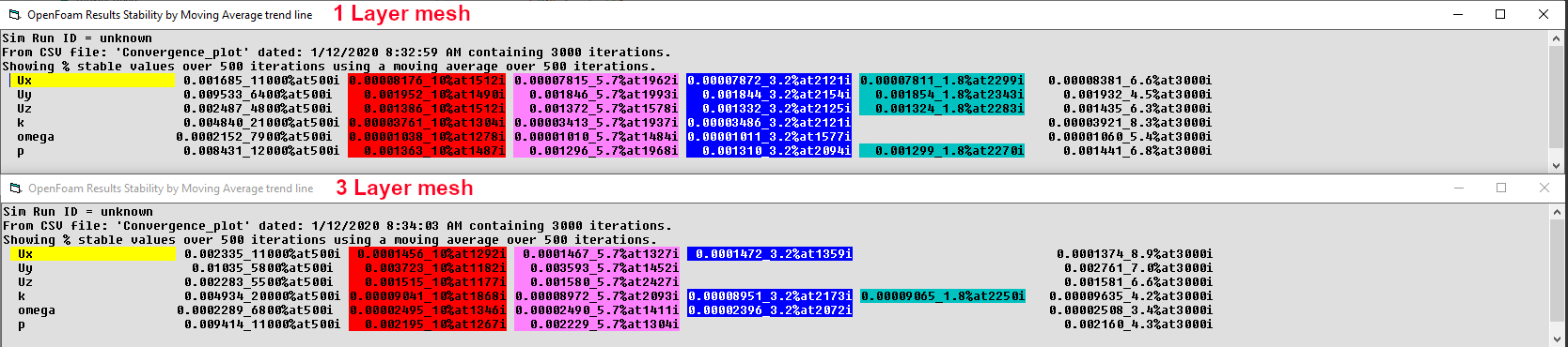
Even at 3000 iterations, both of these meshes’ sim runs have result values oscillating over about a 10% range…
So while we can predict a good single filtered value with ORSI, the solution sets will not represent data that represents those ORSI values… This means that my U magnitude images (based on solution set values at exactly 3000 iterations) WILL NOT SHOW WHAT WE EXPECT and in this case perhaps only within ±5%
Here are those U magntude images at iteration 3000 (with the ORSI values at 3000i shown AND the percent variation from ORSI of the solution set data values at 3000 iterations…
This is just a caution post for when images from solution set data is presented…
.
.
.
. EDIT: And even more importantly, this justifies the need to have ORSI… By that I mean, in the past people are generally just using the result values from the last iteration in their solver log when they say for instance that the CD of my sim results was 0.5 (or whatever). They likely even say that the results were stable without really knowing whether they were or not… They do not realize that if they stopped their 3000 iteration run just 15 iterations earlier the solver log could report at CD of 0.45 from the same run… (not so good is it)…