Introduction
The Moving Reference Frame (MRF) approach is a steady-state method employed in industrial Computational Fluid Dynamics (CFD) to model problems with rotating parts. It is considered to be less computationally expensive and yet accurate enough for most industrial problems.
The underlying physics behind this approach is simple, yet elegant. A thin volumetric region of mesh cells is created around the rotating body during the meshing phase. This region is known as the MRF zone.
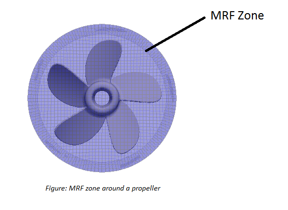
During the simulation phase, the MRF zone is rotated about the axis of the body and the body is kept stationary. In order to preserve the direction of Coriolis Forces on the body, the rotational velocity of the ball is reversed in the MRF zone.
Example Exercise: Golf Ball with an MRF zone
When a gold ball is hit off the tee, it flies through the air with a trajectory controlled by gravity and aerodynamics. Most golf balls have dimples which create a thin turbulent boundary layer of air that clings to the ball’s surface, decreasing the drag on the ball by half compared to a smooth ball.
The dimples also affect lift which is created by the spinning action of the ball. A spinning ball has a higher air pressure on the bottom than on the top which creates the upward force on the ball.
A high fidelity computational study of a spinning golf ball moving through the air requires a quick and robust approach. This is where the Moving Reference Frame (MRF) method comes into play. Rather than “moving” the mesh which would create a high computational effort, we directly add the rotation of the air by adding a secondary volume (the MRF zone).
In the case of the gold ball simulation, the ball is considered to be stationary and an additional volume around the ball is assigned a constant speed of rotation to represent the air domain. You can read more about Rotating Zones in the SimScale Documentation.
In this exercise, you have been provided with the the geometry of a golf ball with an MRF Zone. Your task is to create the mesh, setup the simulation, and view the results.
This project is the starting point for your simulation. Please copy it to your browser:
Mesh Generation
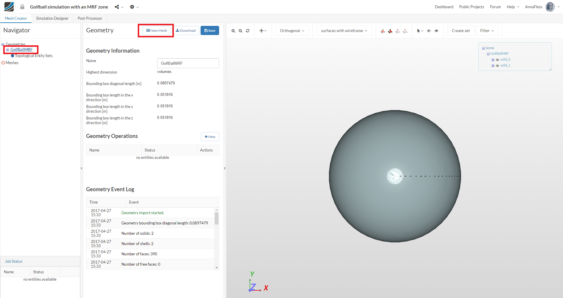
You will notice in the viewer that the geometry consists of 2 solids:
Solid_0 is the MRF zone surrounding the golf ball
Solid_1 is the golf ball
Click on the geometry GolfBallMRF and click New Mesh to create the mesh.
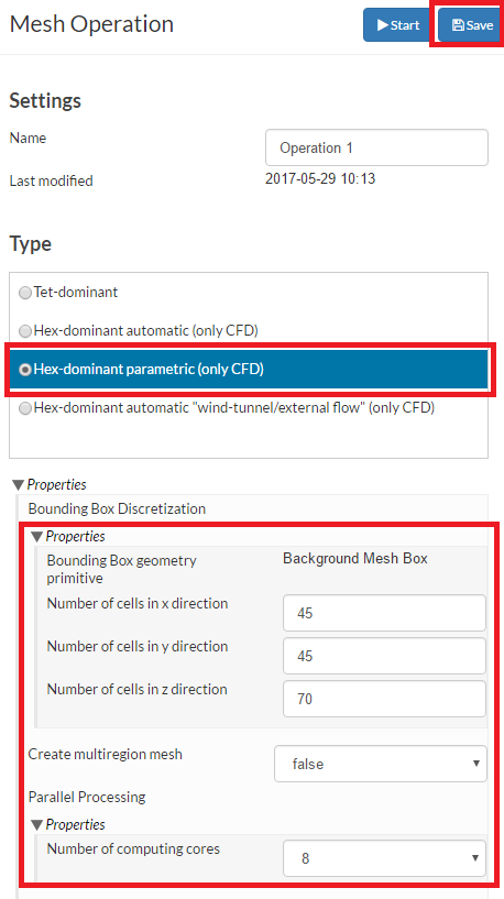
In the middle column select the mesh type Hex-Dominant parametric (only CFD) and set the following parameters:
- Number of cells in x direction = 45
- Number of cells in y direction = 45
- Number of cells in z direction = 70
- Create multiregion mesh = false
- Number of computing core = 8
Press Save
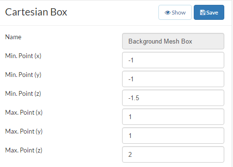
Since we are not able to simulate an infinitely large domain, we must define the air domain around the golf ball. Click on Background Mesh Box and set the following parameters:
- Min. Point (x) = -1
- Min. Point (y) = -1
- Min. Point (z) = -1.5
- Max. Point (x) = 1
- Max. Point (y) = 1
- Max. Point (z) = 2
Press Save
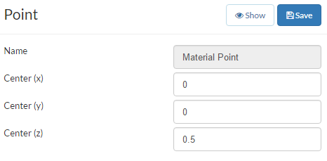
Next go to the Material Point and set the coordinates accordingly:
- Center (x) = 0
- Center (y) = 0
- Center (z) = .5
Press Save
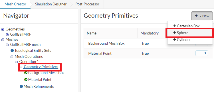
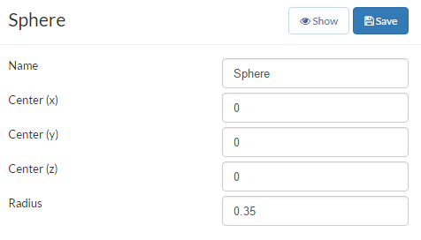
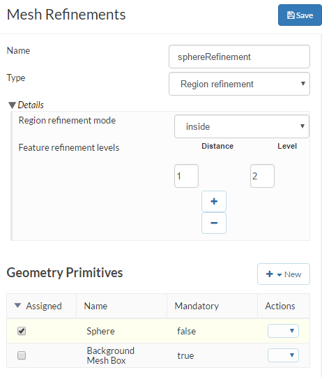
Now, we will add a spherical geometry primitive which will be used later to define a region refinement. Click on the Geometry Primitive item and then +New
Set the coordinates accordingly:
To get a good quality mesh, we will add mesh refinements
Mesh Refinement 1
Click on the Mesh Refinements in the Navigator and then +New
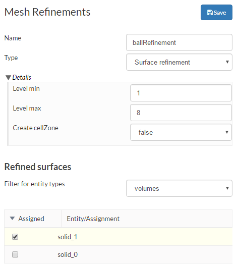
Mesh Refinement 2
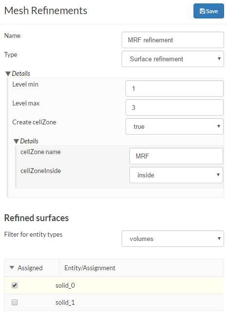
Mesh Refinement 3
To enable the creation of the MRF Zone, we must add a surface refinement to solid_0 and set Create cellZone to true
Navigate to the Operation 1 in the Navigator and Start the meshing operation. The meshing operation will take ~ 10 minutes
Simulation
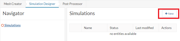
Once the meshing operation is finished, the mesh will automatically load in the viewer. To set up the simulation, move to the Simulation Designer tab
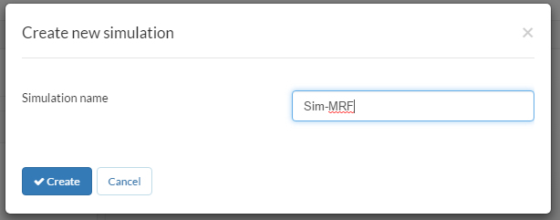
Click +New to create a simulation
Name the simulation setup to Sim-MRF and click Create
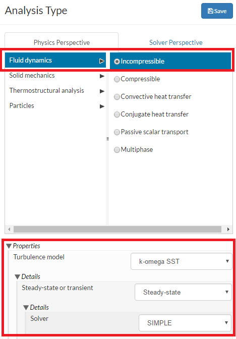
Set the Analysis Type to Fluid Dynamics → Incompressible with the following properties:
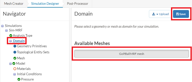
Set the Domain to GolfBallMRF mesh and click Save
Next, go to Materials in the Navigator and +New.
Click on Import from material library and select Air
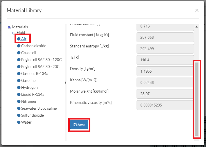
Assign the material Air to both volumes region0 and MRF_solid_0

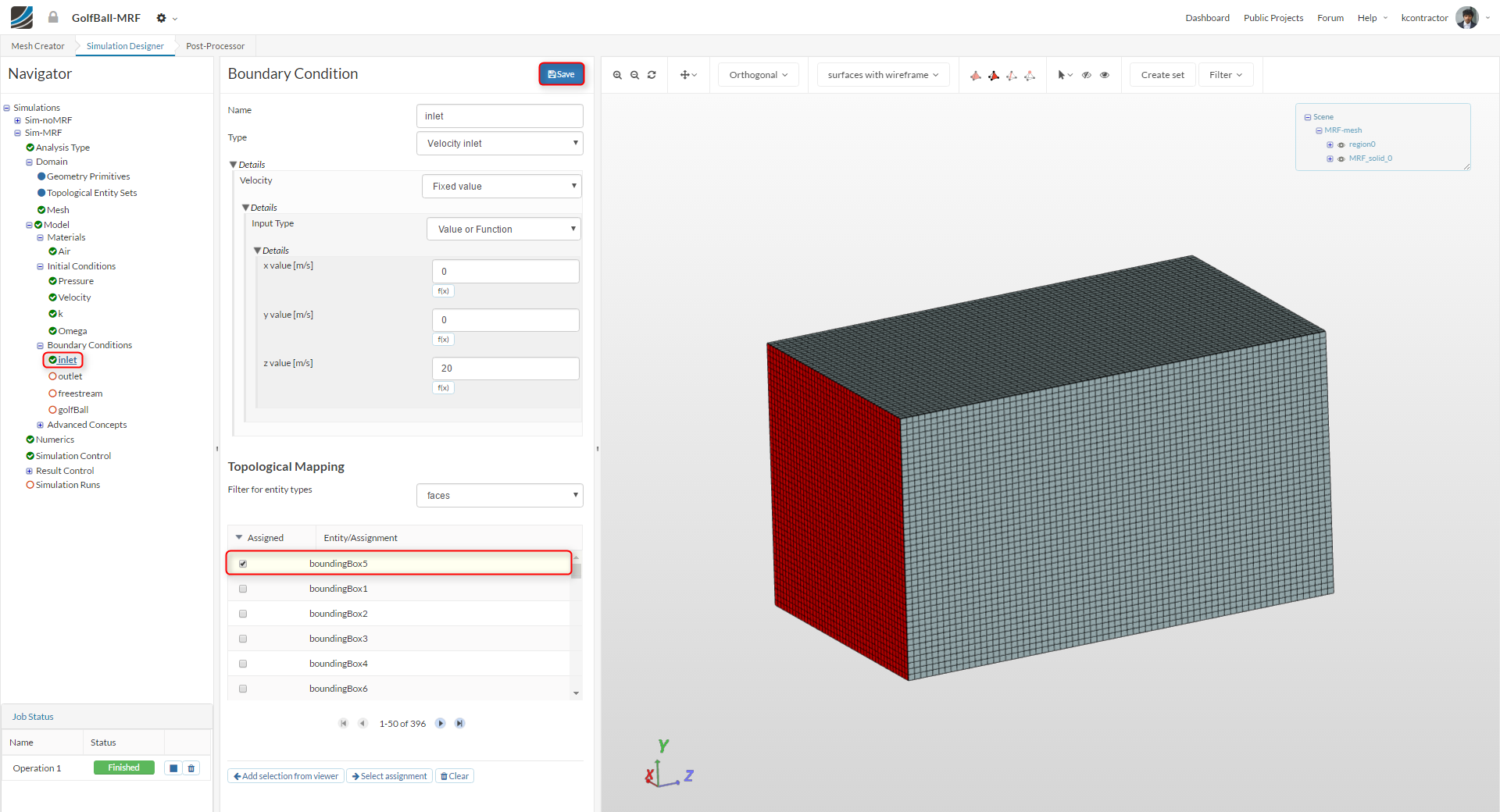
Next, we will set up the Boundary Conditions. Click on Boundary Conditions in the Navigator and then +New
inlet
outlet

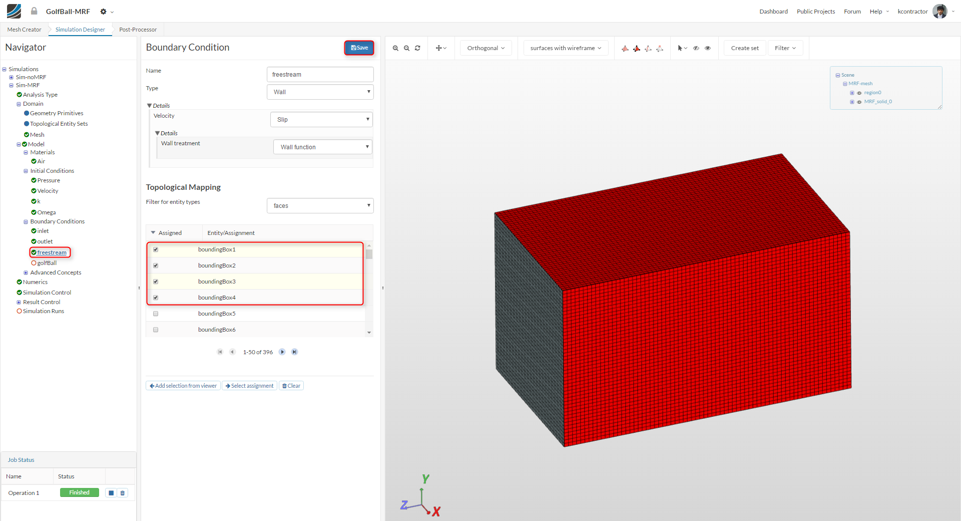
freestream
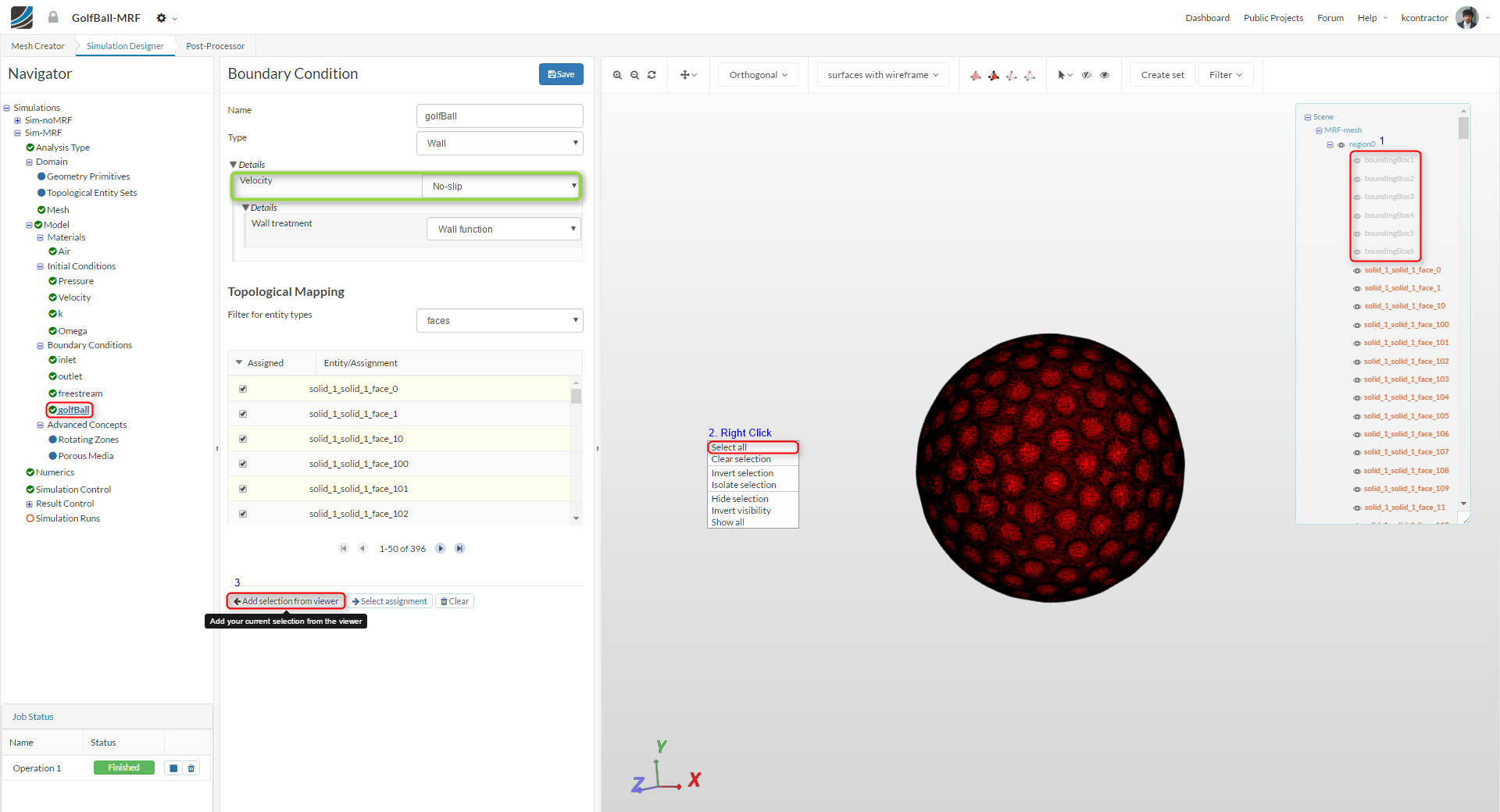
golfBall (walls)
Set the wall to No-Slip. Assign it to the ball by toggling off the visibility of the MRF zone and the bounding boxes followed by selecting all surfaces of the ball and Add selection from viewer.
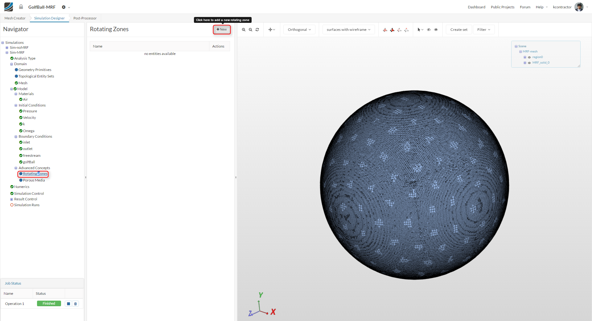
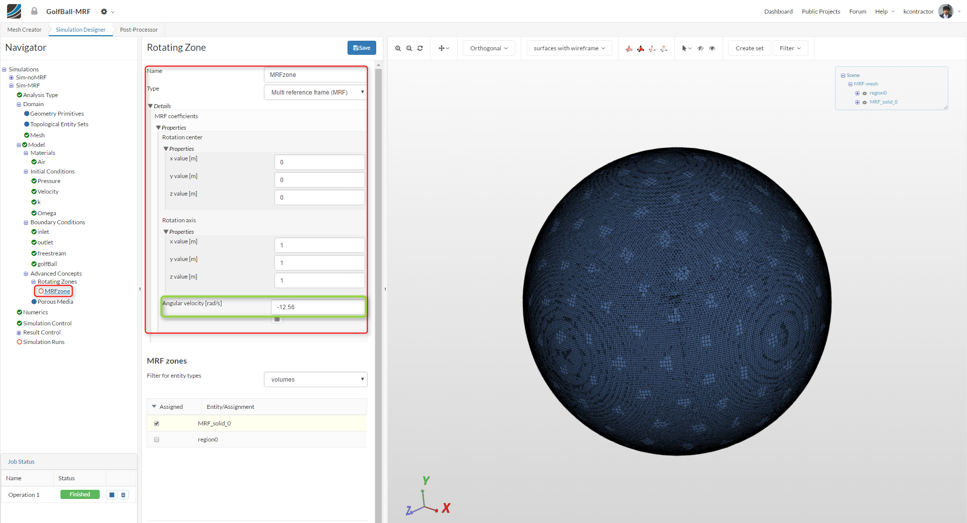
Rotating Zone
Now create a Rotating Zone under Advanced Concepts by clicking on +New :
Since we treat the ball as being stationary in air and the MRF zone around it as a rotating one, the angular velocity assigned should be opposite of that of the spinning ball. Assign an Angular Velocity of -12.56 rad/s to the MRF zone.
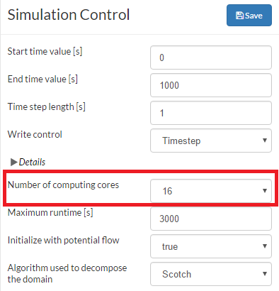
Next, go to Simulation control and increase the number of computing cores to 16
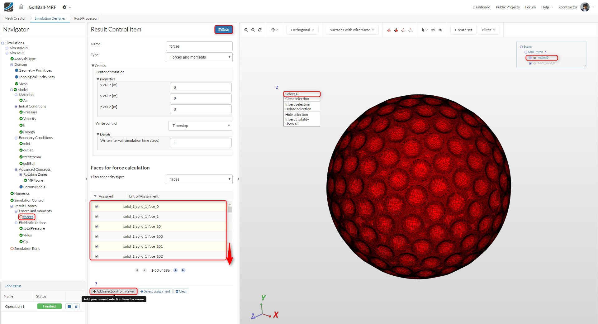
Finally, we can add a Forces and Moments item under Result Control to obtain the lift force acting on the Ball.
Finally,
Create a New run and Start:
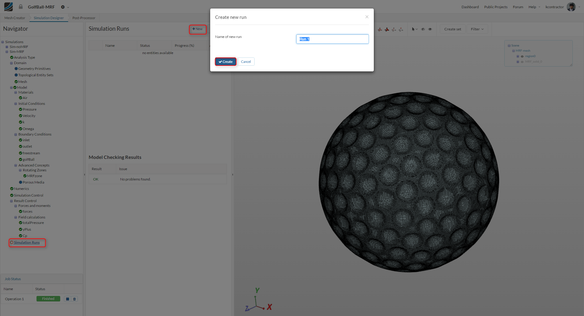
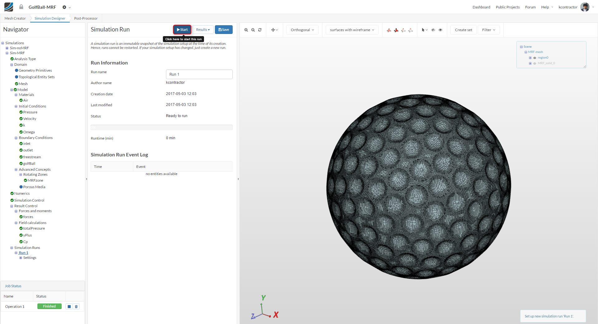
The simulation will take ~15 minutes to complete
Post-Processing
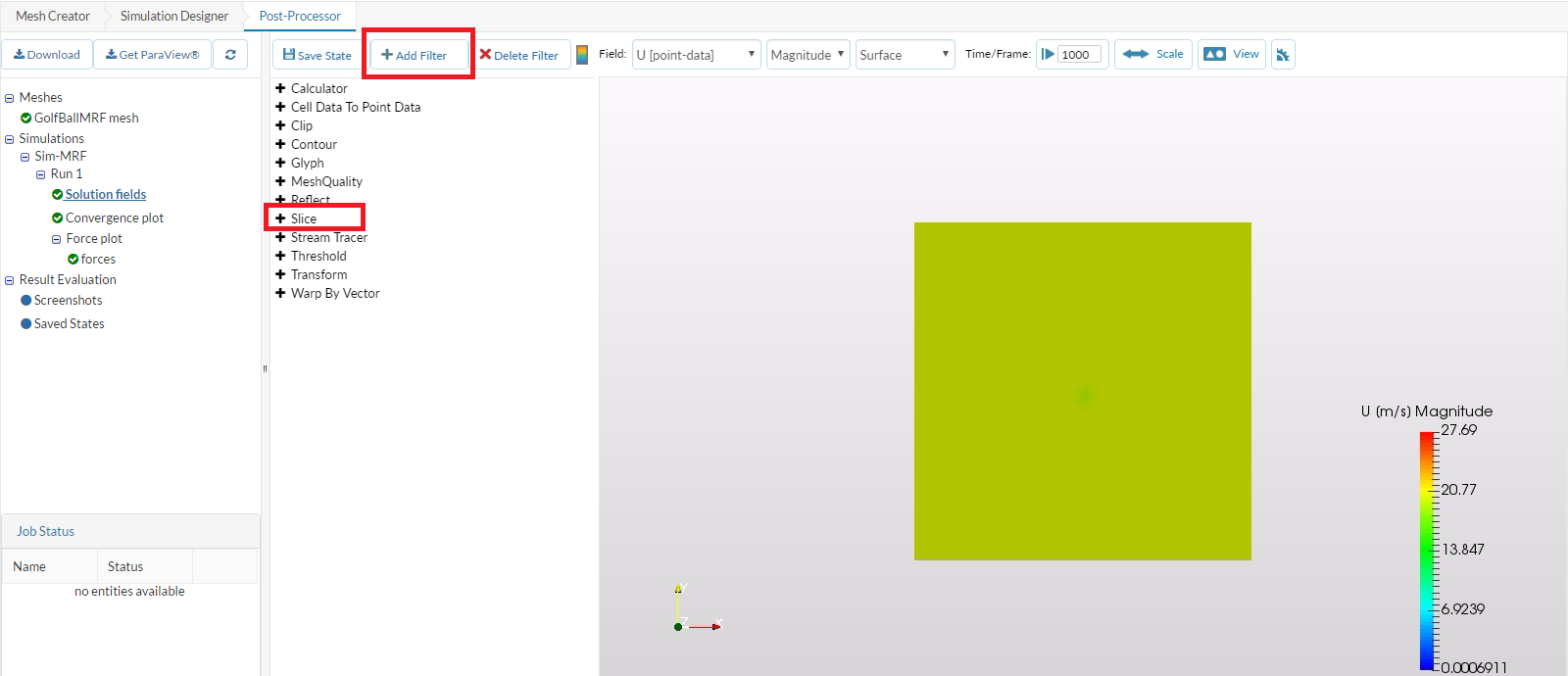
To view the results of the simulation, go to the Post-Processor tab and click on the Solution fields item in the Navigator.
Go to +Filter and select Slice to insert a domain slice to the viewer. The internal mesh is automatically hidden when the slice is added.
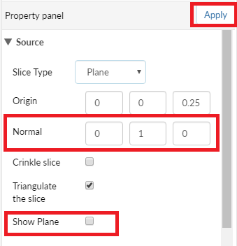
In the Property panel, change the following settings and click Apply
Rotate the slice in Viewer so you can visualize the velocity fields (U [point data])
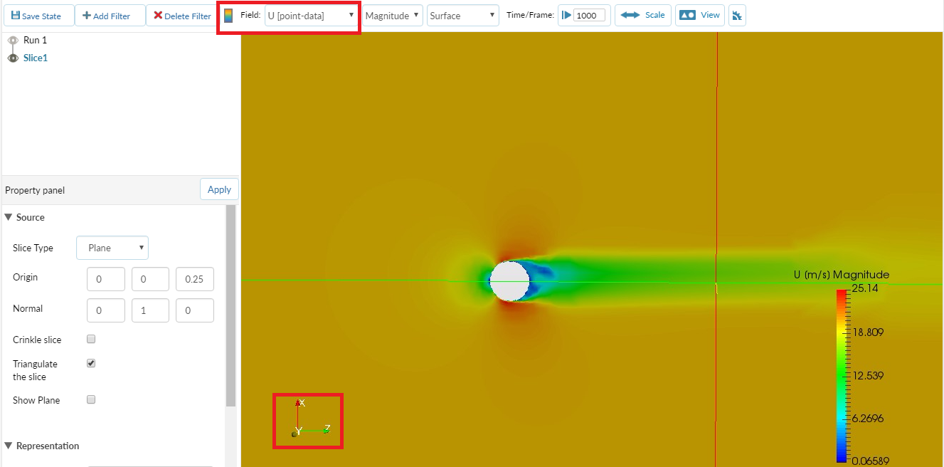
What are your observations about the results?