Fine Tuning Boundary Layer Thickness
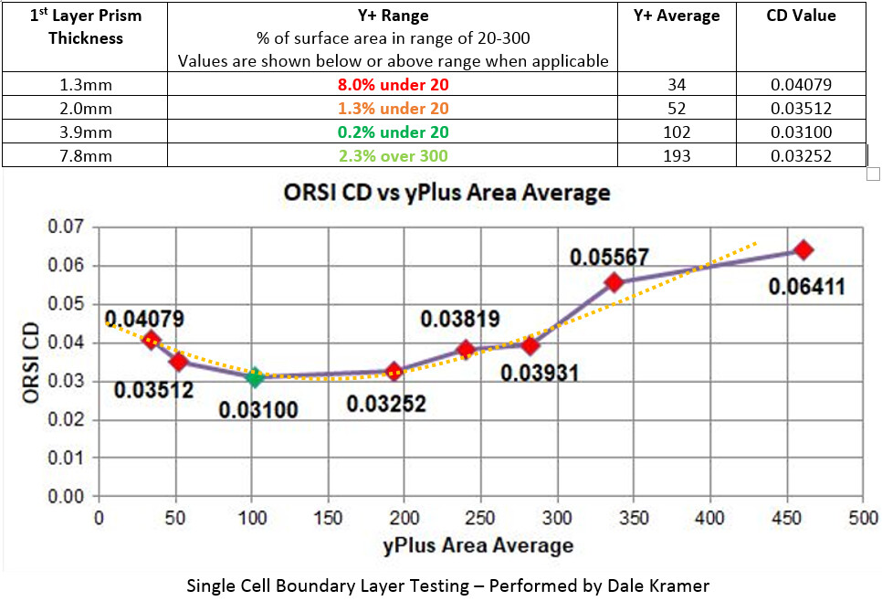
With the success of the short Non-Orthogonality study, the next round of testing was done to confirm that lowering the single cell thickness would have acceptable Y+ values. Through the validation of the single cell boundary layer method, a range of first cell thicknesses were found where Y+ values would fall into the Log-Law region, in addition to cell sizes that would cause Y+ values outside this region. The testing done by Dale Kramer inspected a single cell thickness of 1,3mm up until 31,3mm.
Concentrating on the lower range of his tests at 1,3 – 2,0 – 3,9 – and 7,8mm, a clear trend results where Y+ values were falling in, or out of, the Log-Law region. This can be more clearly seen in the following table.
Using this data, it is clear that the optimal range seems to be between Y+ average area values of 50 to 200. This means that there will be a range of cell thicknesses that will be acceptable for use and will allow a modification of the first cell size in order to solve the layer deflation problem described in the first section. Up until this point, I have only used 3.2mm as my boundary layer thickness for almost all of my FULL CAR simulations, as layer deflation was never a problem in combination with a level 8 - (0,001953m) surface refinement cell size. However, the layer deflation problem started with the level 9 – (0,0009765m) local cell size described above. Now I believe that the single cell thickness can be optimized to further improve mesh and simulation quality. The next set of tests were then conducted to verify the reduction of the single cell thickness for useable Y+ values and to investigate the effect on quality results.
Finding Initial Y+ Values
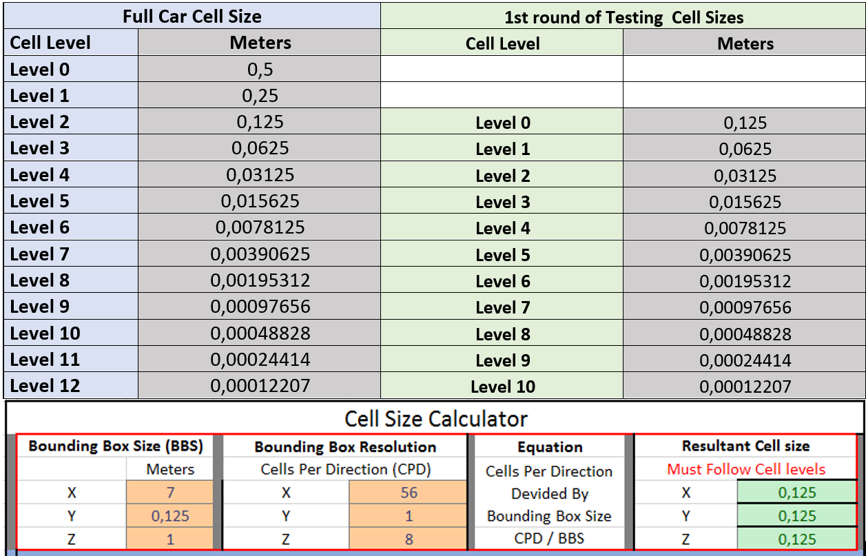
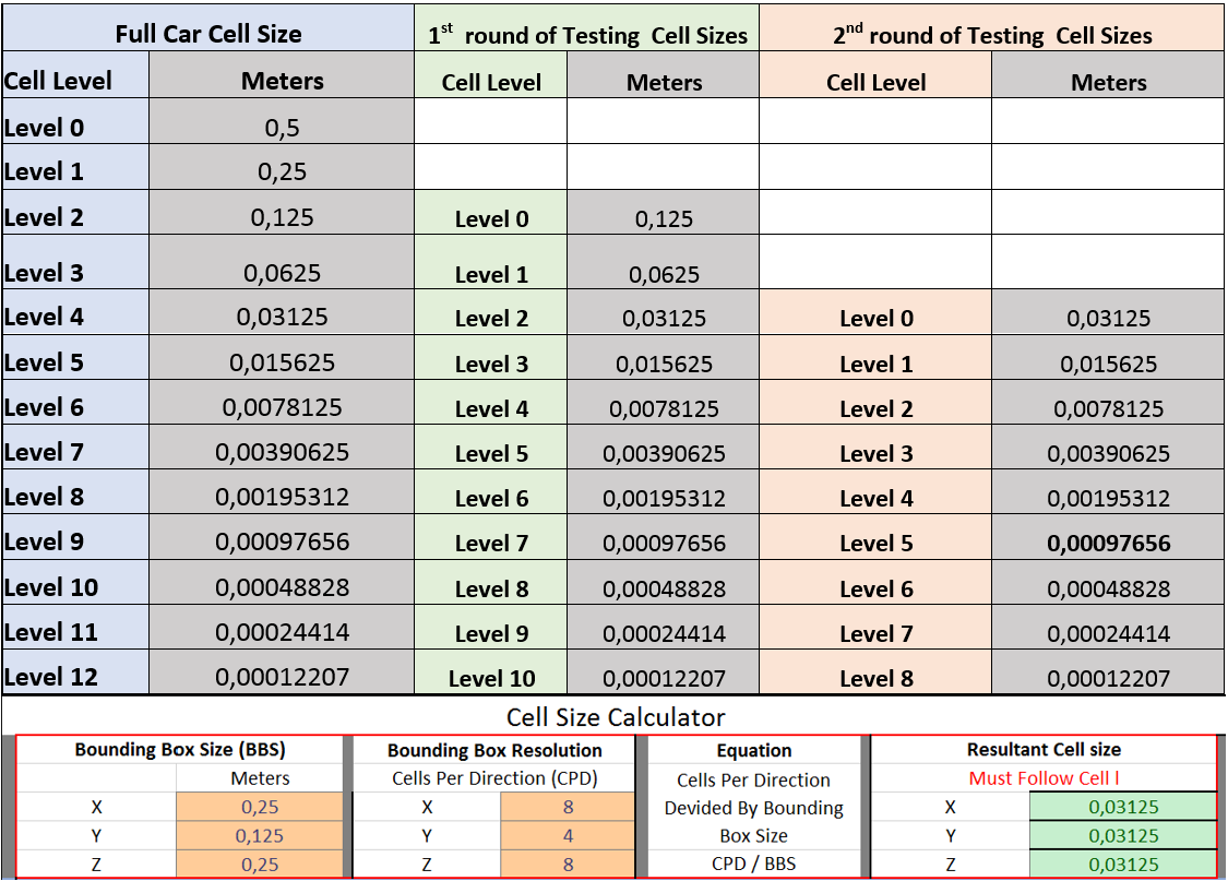
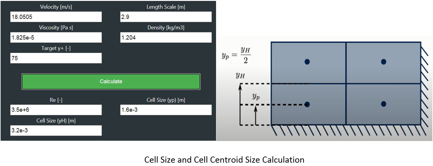
The first step is to use a Y+ calculator to get an initial estimate of the needed first cell size. It is very important at this point to understand that most calculators will output the CELL CENTROID SIZE . This means that the cell size used in the boundary layer refinement must be DOUBLED in order to get the Y+ value calculated. The absolute best description into finding initial Y+ values is from the Fluid Mechanics 101 Video here: https://www.youtube.com/watch?v=60fDz2cVdy8 by Aidan Wimshurst. If you are interested in learning CFD, his channel is a MUST. Using the following settings in his calculator we get an initial cell size (yH) of 0.0032m based off a desired Y+ of 75. The settings are based off of a sea level condition at 20° C.
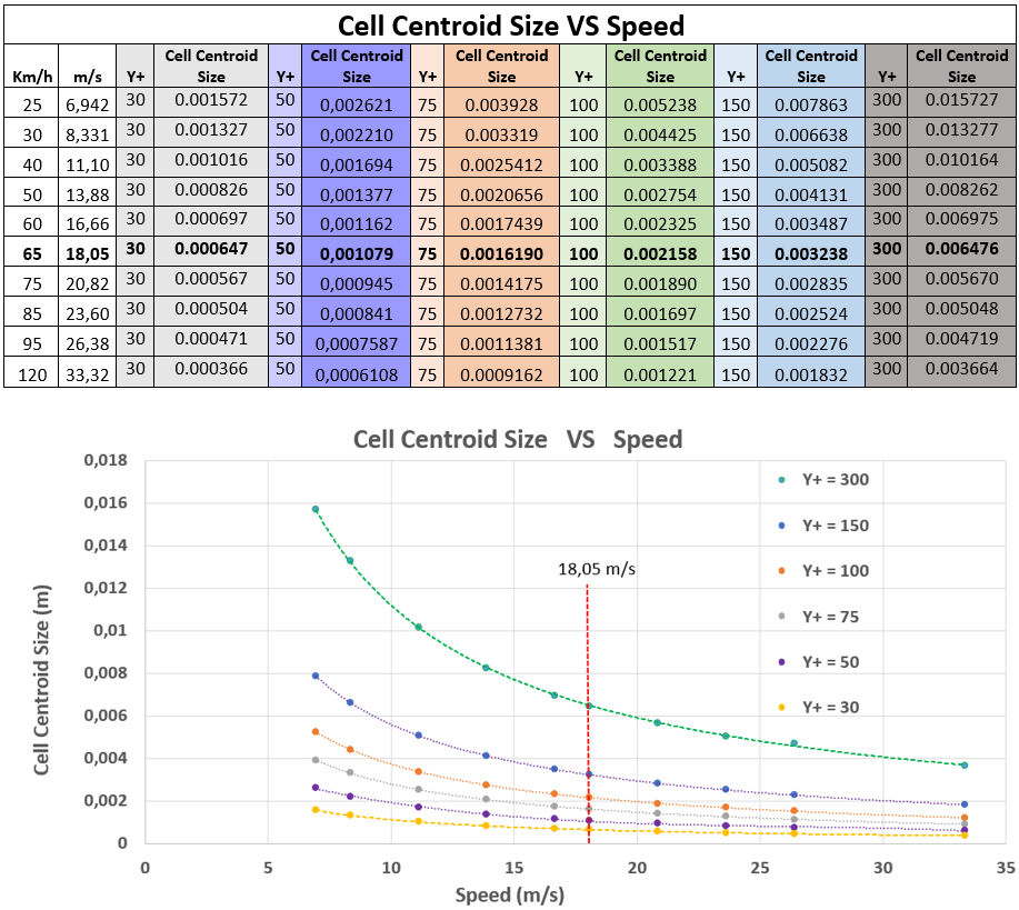
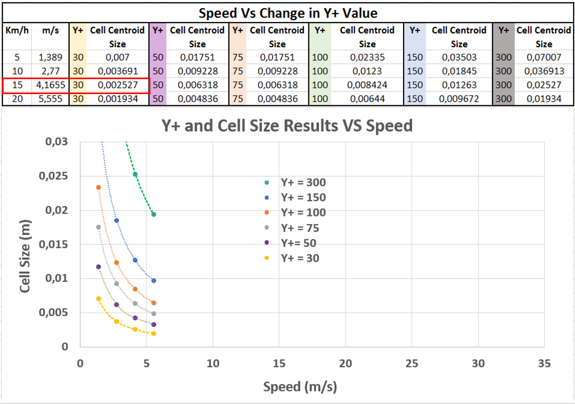
This first cell size from the calculator was the basis for the single cell boundary layer method, however, when simulating at different speeds, the Y+ values will change, and the boundary layer cells must account for this. Shown below are the resulting cell centroid size values based on four different Y+ value inputs, as well as the 30-300 bounding range. It can be seen that with the increasing speed, the required first cell centroid size will shrink. This is because the boundary layer thickness is reduced with an increasing Reynolds number. I will concentrate on 65 km/h as most of my full car testing was done at this speed and because it is the average turn speed of the FSG track.
It can be seen that for a certain speed, there will be a range of cell centroid sizes that will produce an acceptable Y+ average value over the geometry. This is an advantage during meshing because it allows for some modification of the first cell thickness in order to better inflate the boundary layers.
Varying Boundary Layer Cell Size
Testing Round 4
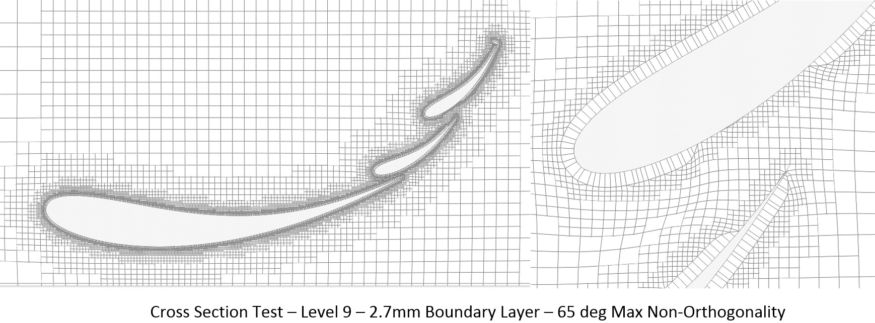
The next round of testing on the very small section geometry started with increasing the boundary layer cell size to 2.75mm, which brought back the layer deflation problem. Even with the Max Non- Orthogonality set to 70, the larger cell size either had too large an aspect ratio compared with local surface cells or created bad snapping points during the layering addition process. Whatever the cause was, this seems to be the upper limit when using a level 9 - 0,0009765m local cell size. I then set the Boundary layer cell size lower, to 2.6mm and the layers returned. They also stayed inflated when I increased the cell size to 2.7mm. Another interesting point is how the quality settings are effected by just the 0.1mm difference in boundary layer cell height.
Testing Round 5
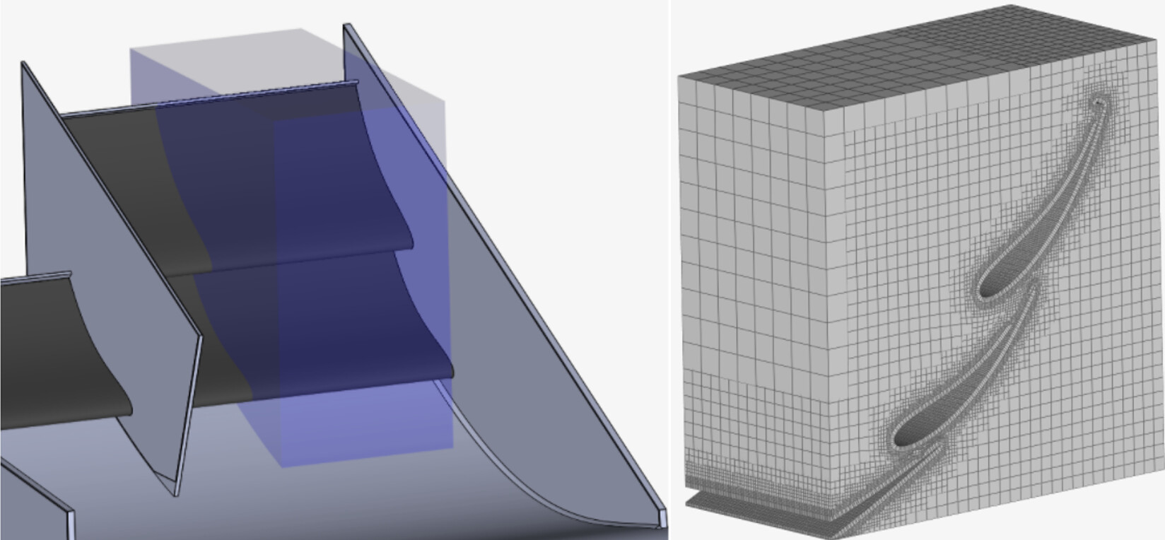
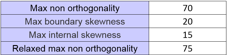
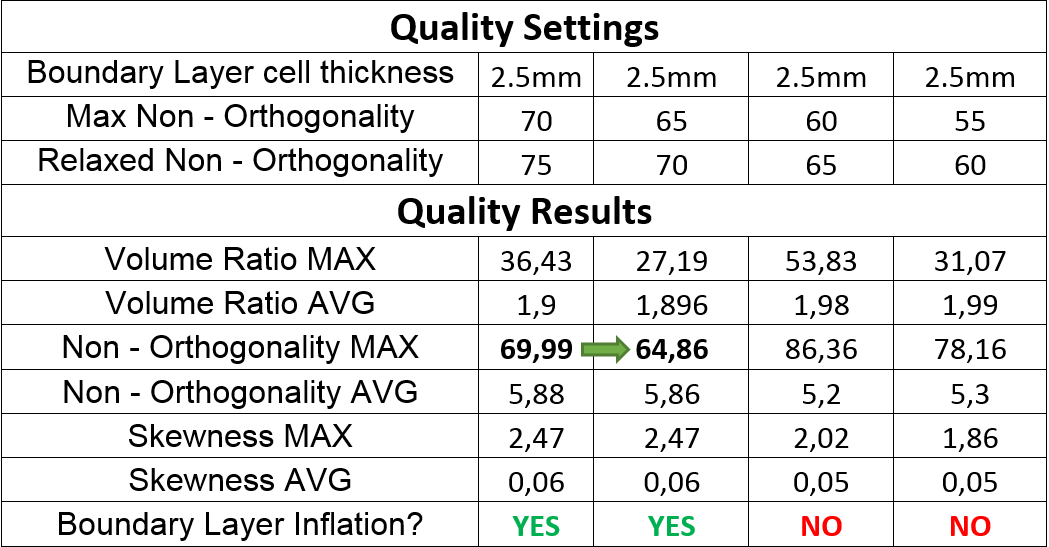
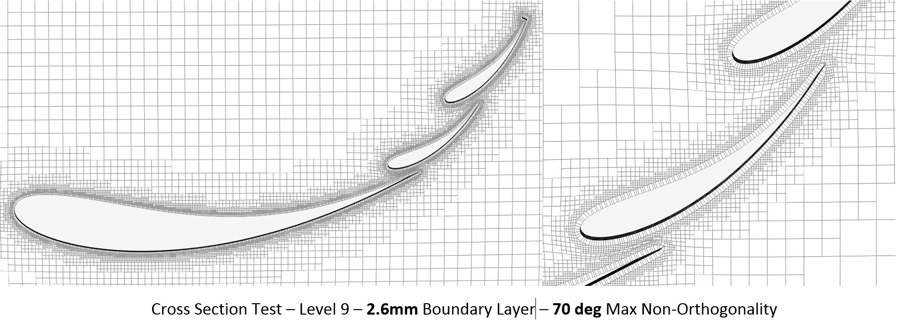
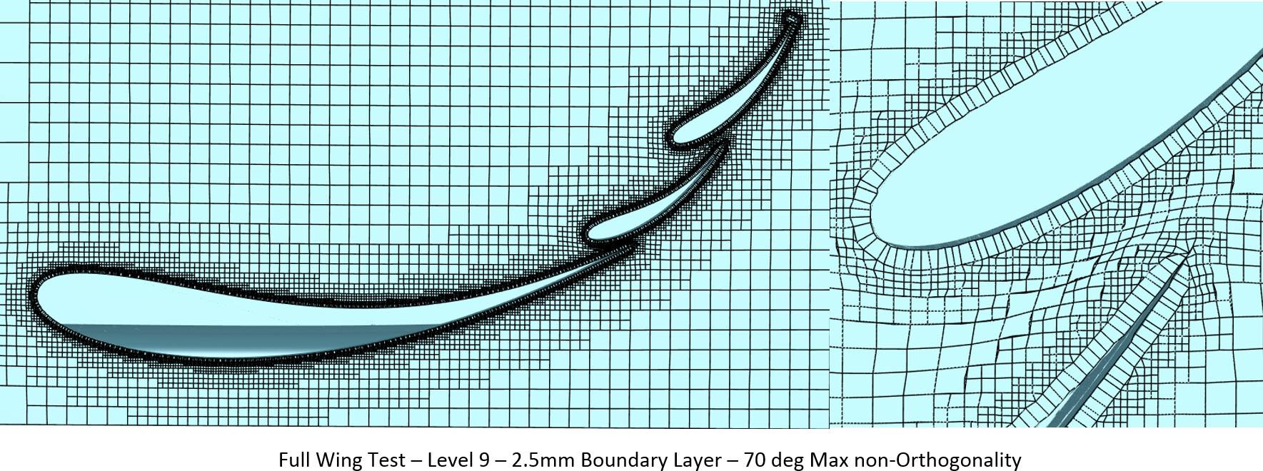
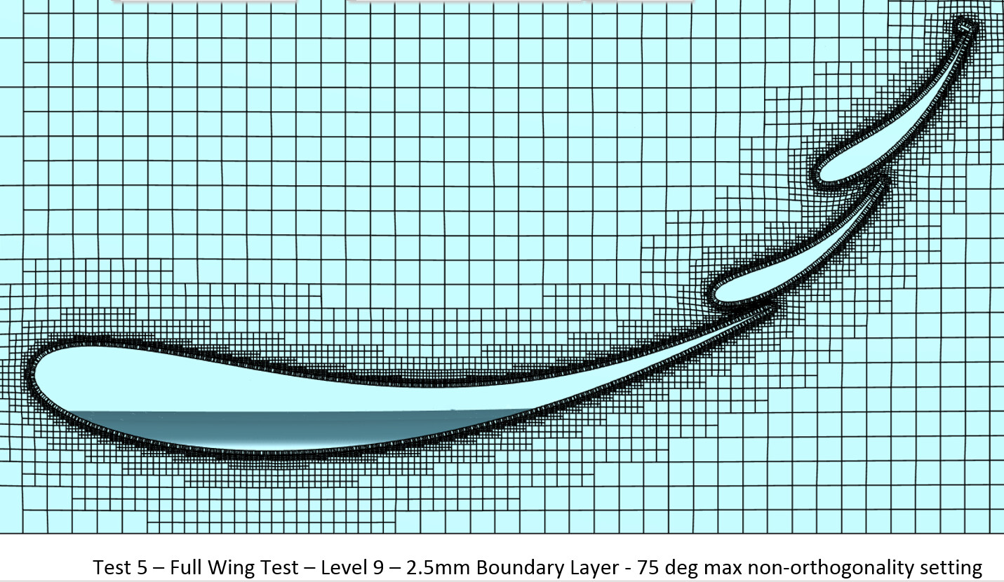
With final testing of the very small section geometry, I moved back to the larger section testing, as presented in the beginning of this article. The best settings from the localized problem area tests in rounds 3 and 4 were used. I decided to go with a 2.7mm boundary layer, right at the edge where deflation occurs, with a 65deg Max non-orthogonality. As you may have guessed, layer deletion occurred, however, this time I knew the solution.
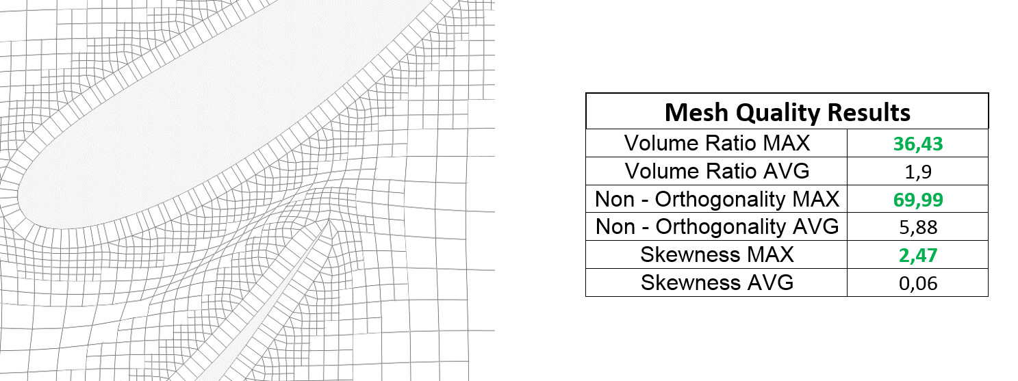
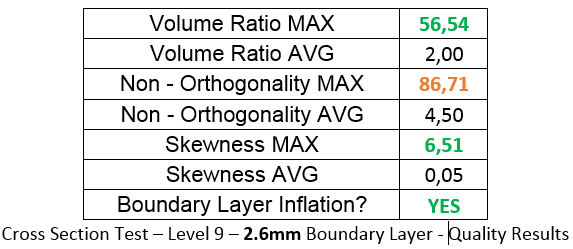
By increasing the Max Non- Orthogonality value to 70, layer inflation was once again present when combined with a 0.0026m thick cell size, producing acceptable quality results.
Reading the Meshing Log
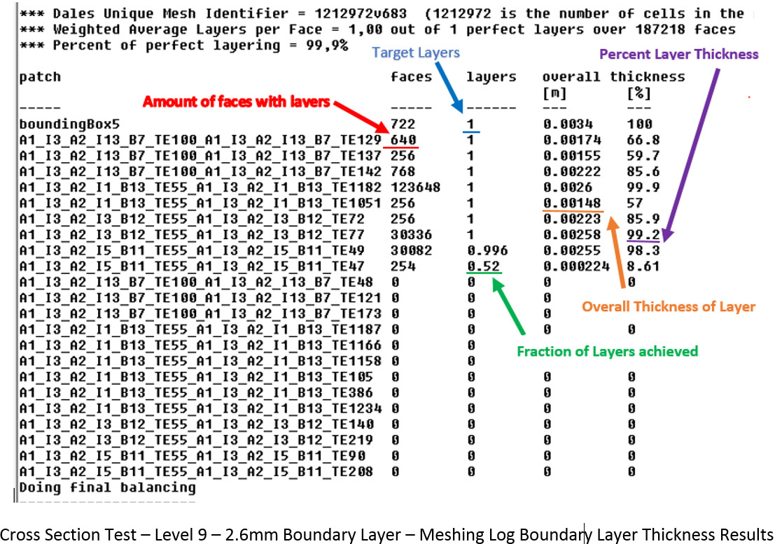
For the run above, it can be seen in the end of the meshing log that the layering results are not optimal. This output shows:
- The amount of faces with layers applied
- The amount of target layers
- The fraction of target layers achieved
- The overall thickness of the layer
- The percentage of layer thickness
This log is also critical to understanding the amount of boundary layers extruded. It will allow you to quickly determine if the Y+ values will be acceptable without running a simulation. A very useful method to save core hours. It can be seen in the meshing log from the “successful” run above that the target number of layers = 1 and is set to 0.0026m. In the layers column, two patches have less than 1.00 full layer, which contributes to a low layer thickness. Looking at the overall thickness, the average of Boundary layer size over all faces is shown. This factor is basically telling us how thick the boundary layer cells are in this area. Even with the achievement of 1 full layer, it can be seen that the overall size does not meet the 0.0026m value that was set in the inflation refinement. This causes the last column, thickness % to reduce below 100. When the layers are not achieving 100% of the cell size (0.0026m) then then our Y+ values will be reduced.
For example, looking at the patch underlined with green, it can be seen that only 0.52 of 1 layer was achieved, resulting in an overall cell size of 0.000224m and a thickness of 8.61%. Looking back at the Cell Centroid Size VS speed results, this would put the Y+ value under 30 for this area of the mesh, over 254 faces. These layer results could contribute to a reduction in Y+ values. The extent of which lies with how far under 100% layer thickness and over how many faces the reduction occurs.
It should also be understood that these values are based on a small cross section test of the wing. With a full car simulation, the amount of faces having lower thickness percentages in comparison to a larger total cell count would make a much smaller impact on the overall Y+ average. Additionally, it is important to understand that WHERE the lower Y+ values are located on the geometry is a critical factor in accuracy of results. This topic will be introduced in the next section. In the end, it is not expected to have a perfect mesh and it is up to you to decide where to draw the line with mesh quality, time invested, and accuracy of results.
Testing Round 6
The next step is to move back into a full front wing test. Starting again using the best known results, a mesh with a 0.0026m cell size and 70deg max non-orthogonality, was created. However, these settings taken from the successful small section test in round 5 again resulted in layer deletion. This goes to show how small section testing success does not mean it will transfer to full scale. By reducing the Boundary layer further to 0.0025m, the layers came back and could be simulated for Y+ histogram calculation.
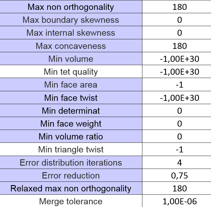
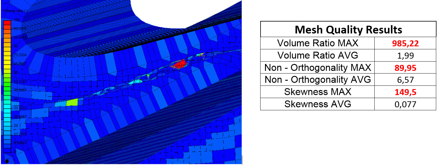
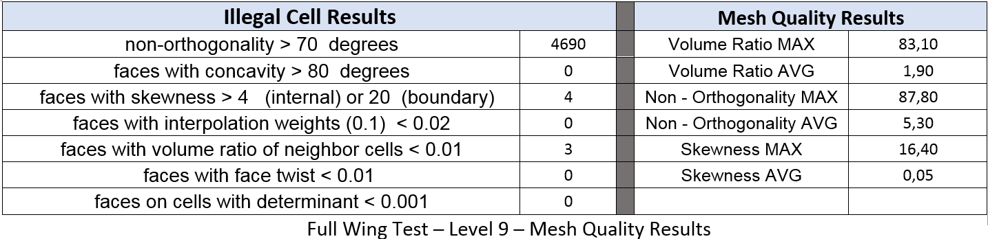
Since I am returning to full scale testing, the amount of Non-Orthogonal cells has increased due to non-boundary layer causes (snapping & geometry related issues). Most of the Non-orthogonal cells are between wing elements (due to cell squish) or where the elements meet the endplates. Reducing these illegals cells can be solved mainly through geometry changes but those solution methods are talked about in the FSAE Tutorial - Preparing Simulations For Success - CAD Preparation article. For this run, the Max and average quality results look good, with Max non-orthogonality a little high at 87 and a few too many illegal cells, but an acceptable starting point.
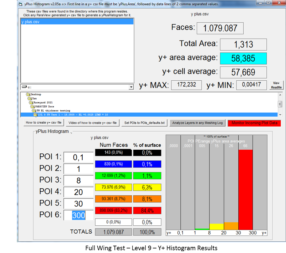
The Y+ histogram results show that there is room for improvement. However, without a visual inspection of Y+ values on the geometry surface, it is difficult to say exactly where these values are located. If they are in areas of low importance and will not have large impact on the results, then the mesh can be used for simulation. The level of quality or percentage of Y+ values in the log law region is once again dependent on what you find to be acceptable for use. In general, the most important area to focus on for an aero foil is the trailing edge of the suction side. This is because it is where flow separation occurs, so accurate measurement of the boundary layer (i.e. correct Y+ values in this area) are required. In the level 9 histogram below, the percentage of Y+ values between 30 & 300 was 84,4%. While this can always be improved, the amount of work and testing to achieve better values could be substantial.
Visual Analysis
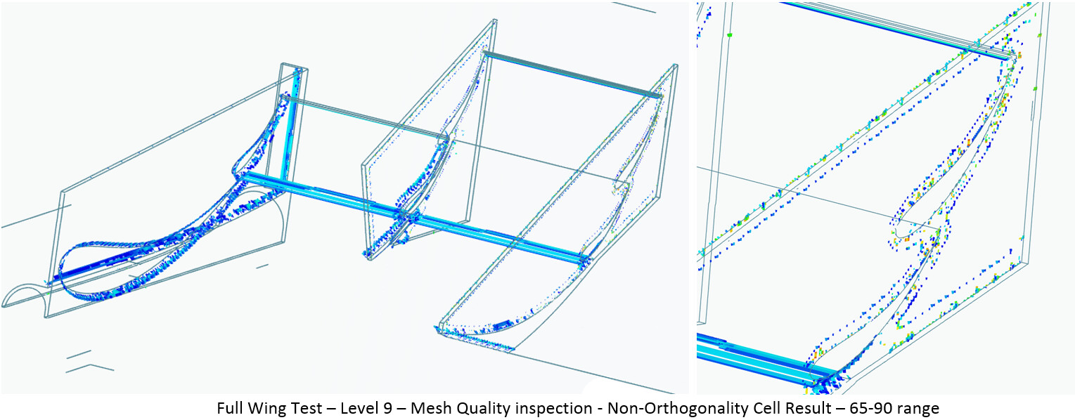
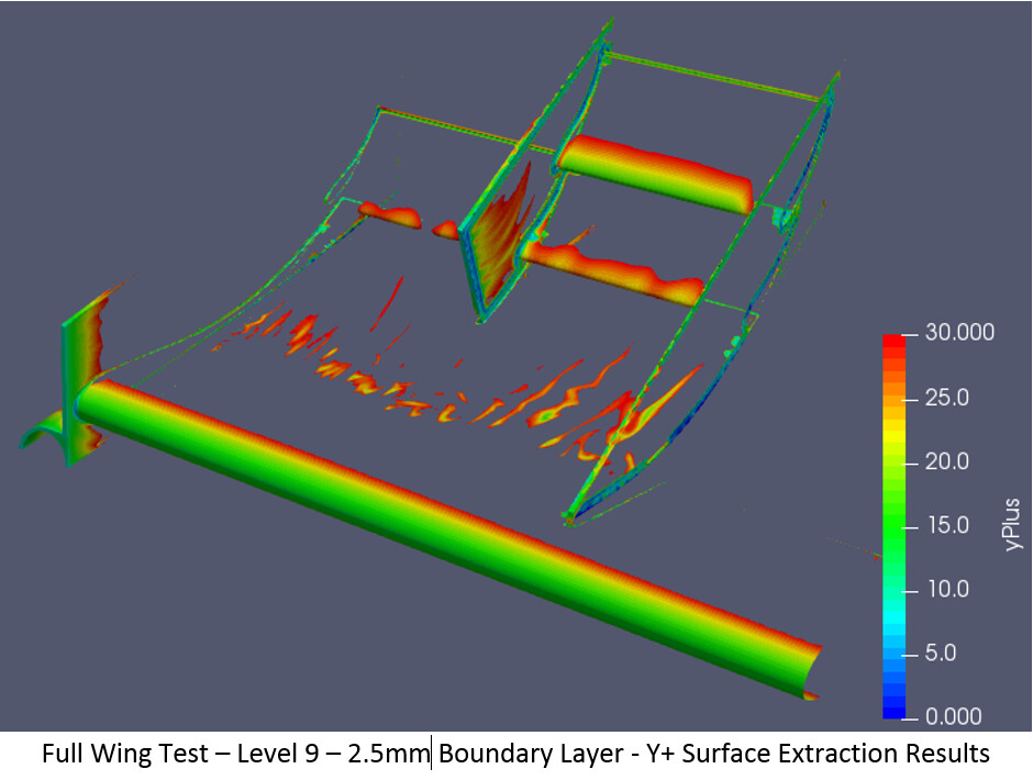
This is where a visual inspection will help to determine if the low Y+ values are occurring in important areas or not. Using Paraview, I applied the threshold feature to extract Y+ values in the range of 0-30. As you can see, most of the Lower Y+ values are occurring at the leading edge of the Front wing and elements, outer endplate, and along the edge were the wing profiles meet the endplates.
I would account these low values to illegal cells in this area. Going back to the quality results picture above, the non-orthogonal cells are also located in these exact spots. Therefore, I can conclude that reducing illegal cells with geometry changes can help increase Y+ values in these areas.
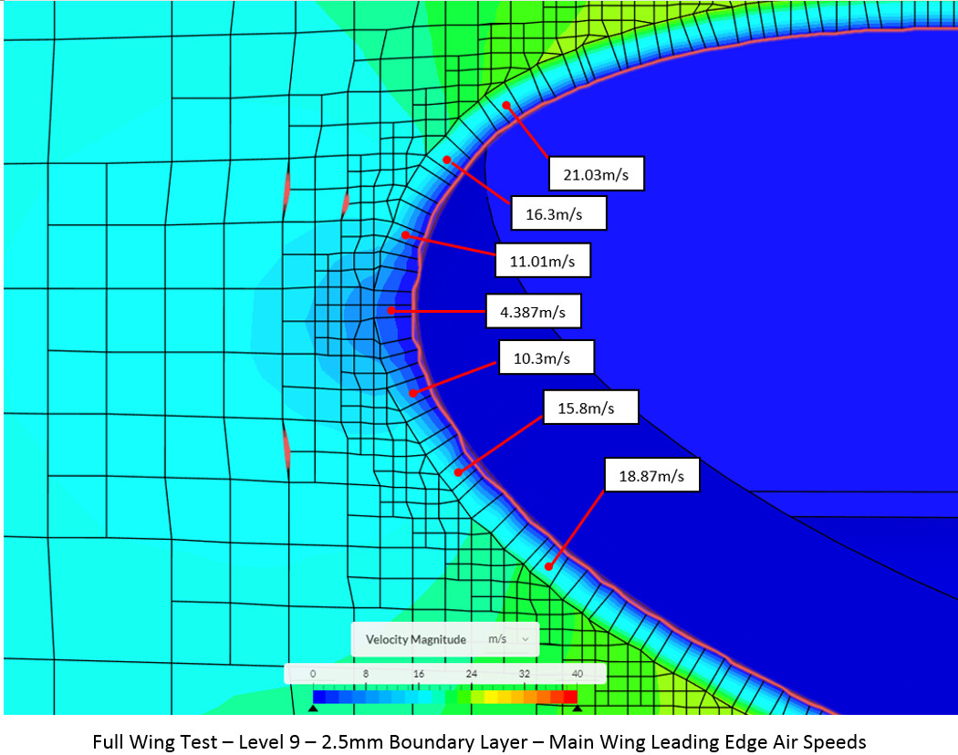
For the Leading edge of the main wing and outer endplate, it can be seen that the Y+ values are much lower than desired – between 10 & 20 – before increasing along the top and bottom of the wing. Since the leading edge of an air foil will have a high pressure region, the air will be moving very slowly. The exact air speeds along the leading edge were recorded from the solutions field.
These values were then added to the calculated results for Cell Centroid size VS speed graph. It can be seen that with low air speed, the target Y+ values result in an increasing cell size requirement. With the boundary layer cells set to 0,0025m (0,00125m Centroid Size) everywhere in the geometry, the Y+ values will be too low at the leading edge and fall close to or under a Y+ of 30. Therefore, the only way to increase the Y+ values in the leading edge, is to increase the current 0,00125m boundary layer cell centroid size to over the Y+=30 → 0,00253m calculated size shown in the red box below. When this distance is doubled to achieve the needed cell size, it means using a 0,005m or thicker boundary layer cell.
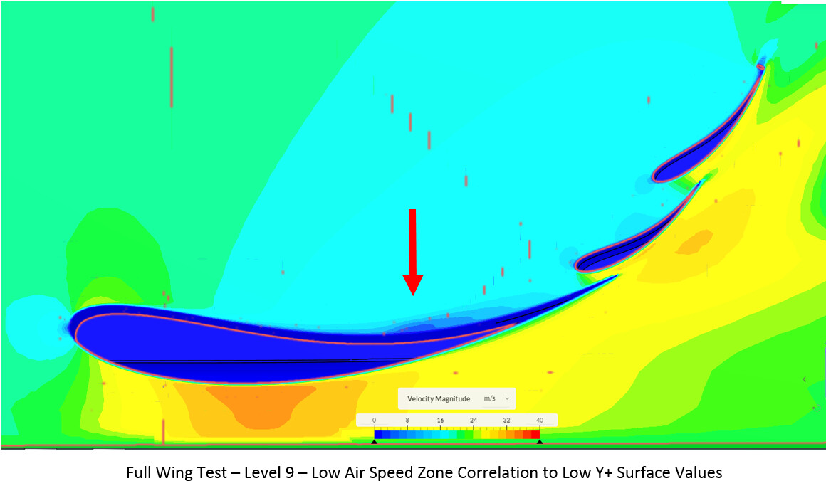
In addition, by looking at the velocity profile over the wing, we can also see a low velocity zone in the middle of the main wing. Looking back at the Visual Y+ surface extraction from Paraview, this corresponds with the “flame-like” zone in the middle of the chord.
The visual Y+ surface results are extremely useful for determining if the simulation can be trusted. With verification that Y+ values are being represented in the correct locations on the wing, I continued testing different settings to try and find a way to increase the overall Y+ values. To do this, I looked into meshing the full wing with a max surface refinement of level 8 (0.001953m) as well. This is because the original goal of these tests was to increase cell fineness of the front wing to see if there was a large difference in force results (a mesh independence test). This project has now morphed into Y+ verification testing, yet is useful nonetheless.
Level 8 Full Wing Testing
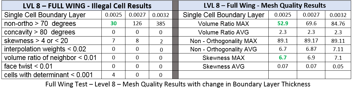
Since the level 9 tests had boundary layer deletion with single cell layer sizes above 0.0025m, comparison testing with the original level 8 wing that used a 0.0032m boundary layer cell could not be done. However, at level 8, boundary layer deletion is less likely and can accommodate a larger range of cell sizes. Therefore, level 8 testing was done at 0.0032m, 0.0027m, and 0.0025m.
From the mesh quality side, there is a clear advantage with a smaller boundary layer cell. The amount of illegal non-orthogonal cells are reduced, as well as the MAX volume ratio and skewness. However, the MAX non-orthogonality remains practically the same.
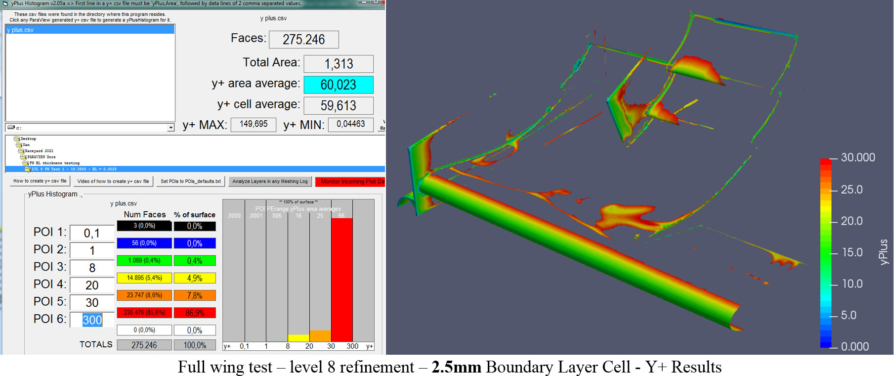
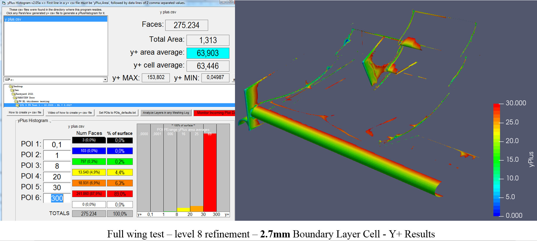
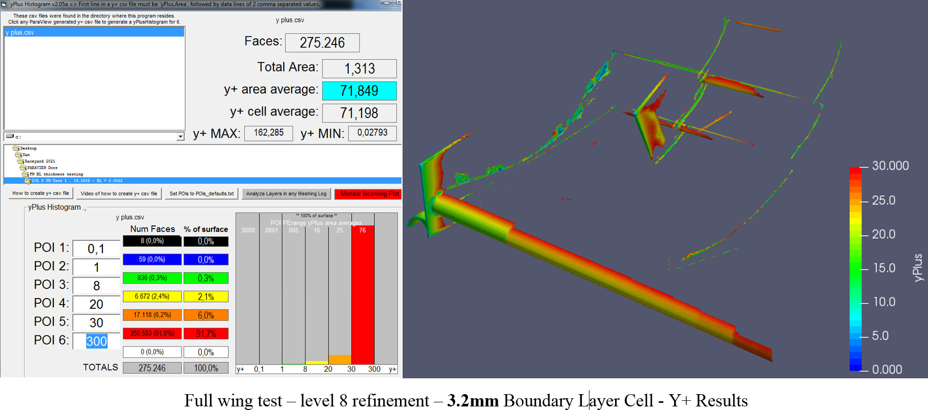
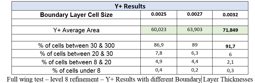
Looking at the Y+ results, the goal is to achieve some Y+ value improvement as all three tests have a decent amount of cells below 30. Only the 0.0032m cell size was able to achieve over 90% of cells in the log-law region. This can be contributed to the thicker boundary layer size being able to remove some of the lower Y+ values around the leading edge of the wing. The thicker cell centroid (0,0016m) can now measure speeds as low as 6-7 m/s, and keep the Y+ over 30. In contrast the 0,0025m boundary layer cell (0,00125m cell centroid) cannot measure speeds this low without the Y+ falling below 30. The limit for this boundary layer cell size is around 8,5 – 10 m/s, meaning the air speed must be above this threshold for Y+ surface results to show values over 30. Looking at the Y+ surface data, in addition to the Histogram results confirms this.
All three boundary layer sizes achieved full layer inflation when inspecting the mesh. It can be seen that the 0.0032m thick BL has the highest Y+ average area and percent of Y+ values in the 30-300 region. Looking at the Y+ surface results for the 0,0032m boundary layer cell, there is clearly an increase in Y+ on the main wing leading edge, as well as other locations throughout the geometry. This result makes it seem that the largest initial boundary layer cell size the better. However, the first section of this article portrayed how difficult it can be to even get full boundary layer inflation on the geometry. For full layer inflation, a thinner boundary layer cell size has clear advantages, in terms of success rate and reduce illegal cell count. Therefore, the balance between these two factors is important, yet once again, is up to you to decide where the line is.
Round 7
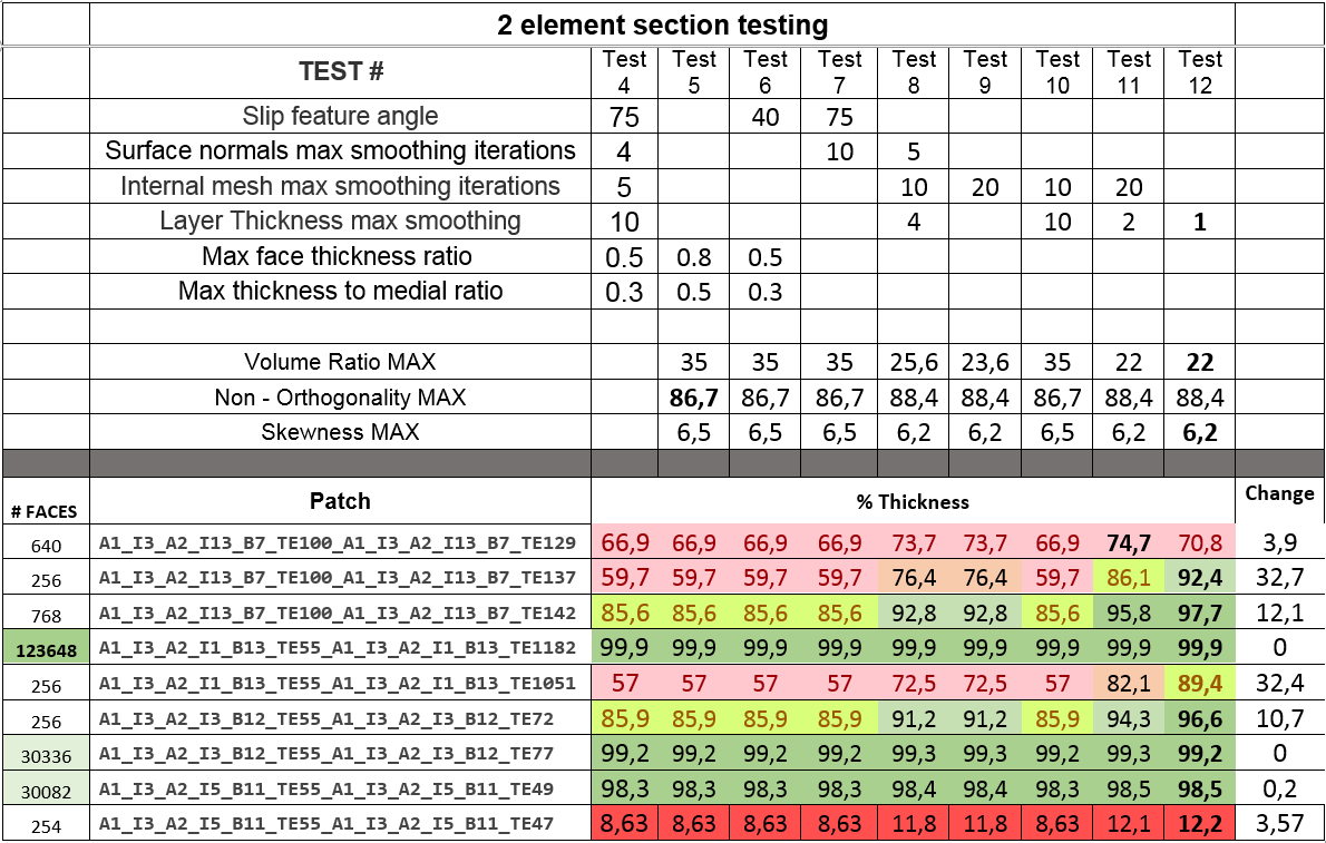
In search of further improvement to layer thickness, I decided to go back to the 2 element cross section test for quick turnaround times and played with some of the layer addition settings until a good solution was found. The changes shown below to these settings in tests 4 - 7 had little effect on layer thickness. Then in test 8, the setting: Layer Thickness Max Smoothing (LTMS) was reduced, which had a very large effect on the end result. With Layer Thickness Max Smoothing set to 1, the section test had the best values, with almost all patches achieving over 90% inflation. For this improvement interpretation, it is important to remember that the amount of faces in the patch can be seen as the determining factor for how critical it is that layers are close to 100% inflated. If there is a low percentage of inflation over a large amount of faces, then the Y+ value will be greatly affected. However, if there is a low inflation percentage over only a few faces, then this can be mainly ignored.
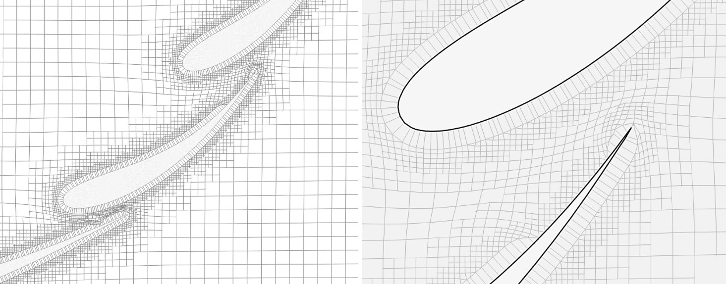
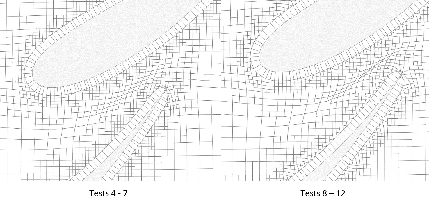
Along with the changes to boundary layer thickness percentage, there were also changes to the resulting mesh quality output. MAX volume ratio was reduced, skewness stayed about the same, yet MAX Non-orthogonality increased. This can be contributed to the layers regaining their thickness and pushing the hex cells further outward from the geometry. This is clearly seen below with the difference in cell squish between wing element cross section pictures for tests 4-7 compared to tests 8-12 shown below.
A “heat map” is applied to the data, with Green representing better values and Red representing worse values. Values in BOLD are the best in the whole data set.
With these successful results, an in-depth investigation into the effects of the LTMS setting was performed. Originally I suspected that the increased thickness percentage of each patch would have a significant effect on the Y+ values. However, this expectation was proven not to be true. Nonetheless, improvements to the mesh can be seen with a lower LTMS value.
Round 8
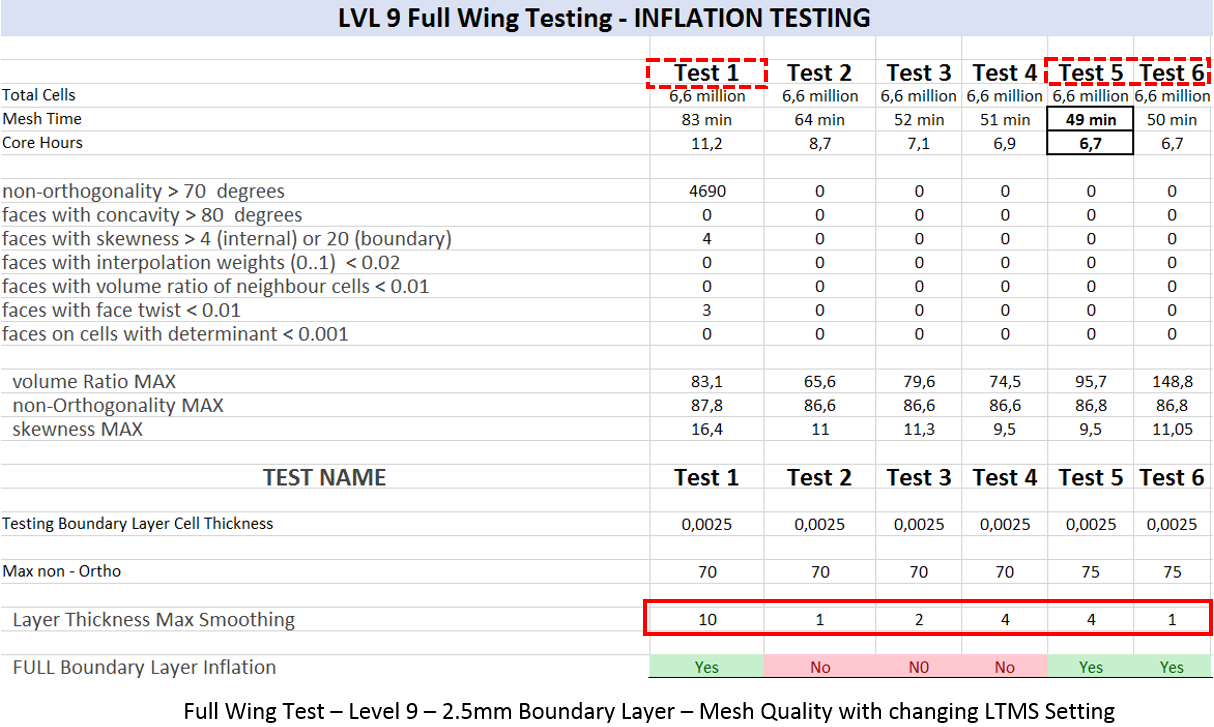
With the new setting found, testing was once again returned to the full wing geometry. Starting with the level 9 full wing, a comparison was made between the layer thickness percentage achieved and the Layer Thickness Max Smoothing (LTMS) setting. Test 1 is copied from the beginning of Round 6 testing and is the baseline for the improvement comparison. The first step was visually inspecting each test for full boundary layer inflation on the geometry surface. Test 2, 3, and 4 had layer deflation with Layer Thickness Max Smoothing set to 1 ,2, and 4 respectively. With this successive failure, Test 5 increased the Max non-orthogonal quality setting to 75, which resulted in the boundary layers returning.
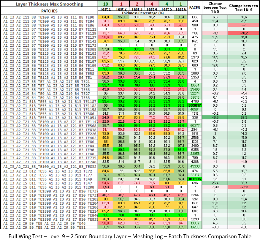
With the success of Test 5, Test 6 returned the Layer Thickness Max Smoothing back to 1, which was also able to fully inflate the boundary layers when the mesh was inspected visually. The next step was to compare the percentage of layer inflation achieved with the change in the LTMS setting. The following table shows this comparison for each patch, including the number of faces, in order to associate the importance of inflation in patches with a high amount of faces.
In addition, interesting results in quality settings and meshing time became apparent. In each test with a lower amount of smoothing loops, the mesh time and core hours required was reduced. This result is not unexpected as a fewer loops for the algorithm to perform will obviously take less time, however, such a drastic reduction in mesh time was not expected. Most notably, Test 5 was almost 2X faster for turnaround time and much lower core hour consumption.
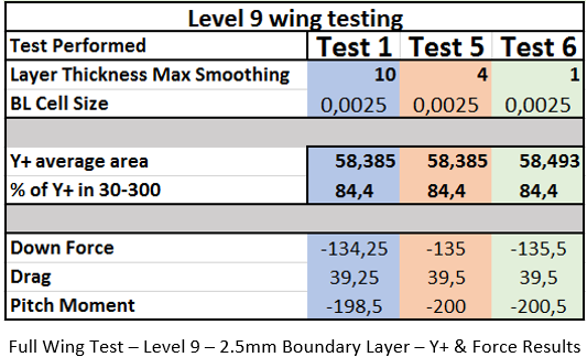
Comparing the results between only the fully inflated runs, Tests 1, 5, & 6, the change between them was mostly positive, meaning each face in the patch was able to achieve a larger percentage of boundary layer inflation. These runs were then simulated, in order to compare the percent of inflation from the meshing log to the Y+ histogram results. The results were fairly disappointing. I had expected that the increased boundary layer thickness shown in the meshing log would have been directly correlated with a higher Y+ average area, and also a higher percentage of Y+ values between 30 & 300. However, the results show otherwise.
Without showing every single Histogram screenshot, I have summarized the three test results into the Y+ average area and percentage of Y+ values within 30-300. Additionally, I have added some force and moment results to show the influence that Y+ values can have on force accuracy. For the level 9 testing, even with the increased boundary layer thickness percentages, the Y+ values from the Histogram show no change. The force results are also fairly similar, other than the pitching moment difference between Test 1 and 6.
Round 9
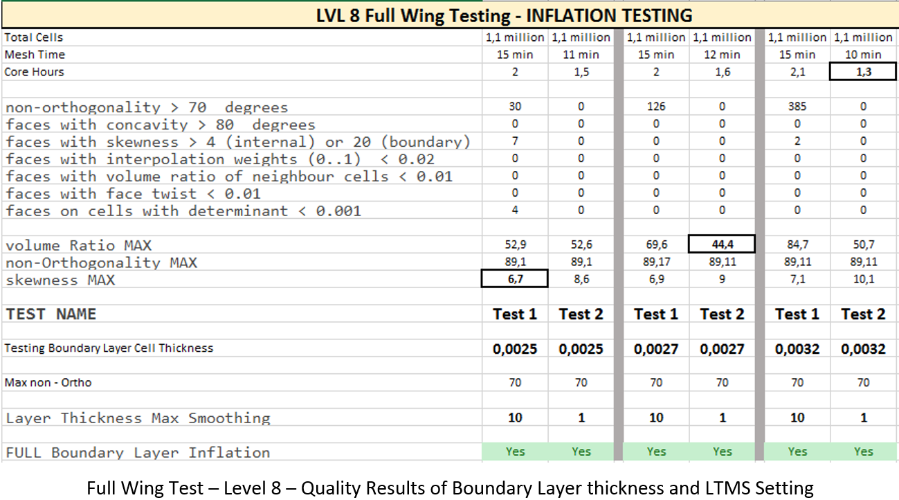
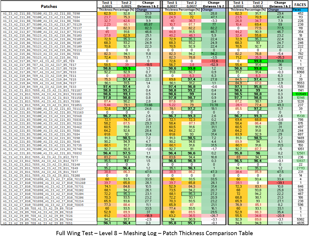
Continuing the testing on the Level 8 full wing geometry, results were fairly similar. This time however, different boundary layer thickness refinements were used to compare not only the effect of the LTMS setting, but also the size of the single cell layer. Boundary layer sizes were tested at 0.0025, 0.0027, and 0.0032m and were ran twice with LTMS at 10 and 1. For the 0.0027 and 0.0032m BL runs, the MAX volume ratio was reduced, for all three tests, MAX non-Ortho stayed the same, MAX skewness increased, and the total illegal cell count was reduced.
Once again, there was an increase in layer thickness percentage between a LTMS of 10 and 1 in the Level 8 full wing tests. However, in this set of runs, the main change in Y+ values was due to the different boundary layer cell thicknesses.
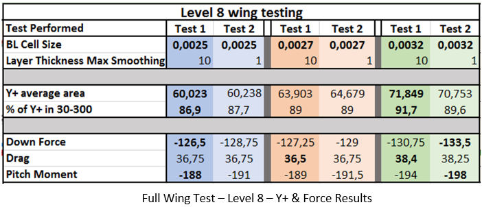
For the level 8 Testing, it was expected that the Y+ average area would increase with the thicker Boundary layer size given. However, the difference between the LTMS values was not as dramatic as I had hoped. What is also interesting, is that the Y+ average area stays relatively the same when switching the LTMS from 10 to 1 for the 0.0025 runs, then increases from 63.9 to 64.67 in the 0.0027 runs, then decreases from 71.85 to 70,75 in the 0.0032m runs. Further analyzing these results, test 1 of the 0.0032m run had the highest percentage of faces in the 30-300 zone at 91.7%. However, the Y+ percent increased between tests 1 & 2 of the 0.0025m runs, stay the same in the 0.0027 runs and then decreased in the 0.0032m runs. Other than the 0.0025m run, this trend correlates to the change in Y+ average area, which makes sense, as an increase in ALL Y+ values should also increase the amount of faces that lie in the 30-300 region, however small.
Moving onto the Force results, a drastic difference can be seen. This causes some concern as the change of 7N of downforce, 1.9N of drag, and 10N of pitching moment can have large effects on wing performance and pressure distribution. In addition, the difference could affect design decisions and wing placement settings, especially with a 10N change in pitching moment.
Now the question remains, what is causing the difference in force results? For the Downforce change of 7N, the highest value of -133.5 came from 0.0032m Test 2, which had a lower Y+ average area and lower percent of Y+ values in the 30-300 range then test 1. This trend is not true for the 0.0025m run, where the higher percent of Y+ values resulted in an increase of downforce. Then with the 0.0027m run, the exact same amount of Y+ values between 30 & 300 also resulted in an increase of downforce. These uncorrelated trends could be from the small testing field, yet a more likely cause, is the fact that I only ran these simulations to 500 iterations. With so many tests performed, I wanted to have a quick testing turnaround time. So the possibility of more accurate results could come from making sure that the simulation has full stabilized. This could be investigated with further testing.
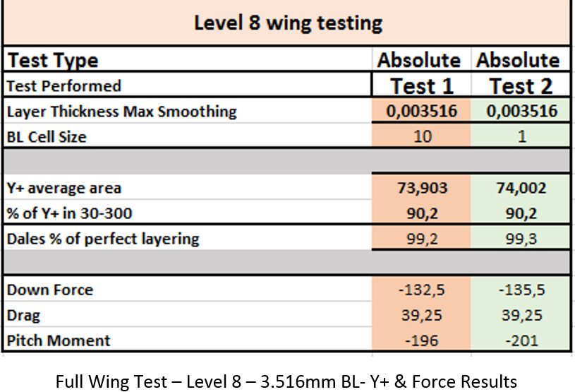
Round 10
In this final round of testing, I wanted to investigate the effects of a larger single boundary layer cell. Therefore, I ran another test at 0,003516m total cell thickness, again with the LTMS setting at 10 & 1. I will leave out the quality results and the patches and layering thickness results as these are the same as all previous testing with better values using a LTMS of 1 rather than 10.
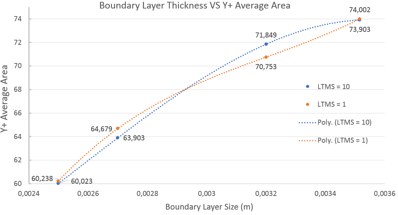
With these results added to the other boundary layer thickness tests, I have made a few graphs to compare these trends. The first graph shows the change in Y+ average area VS the chosen boundary layer cell size. The trend shows higher Y+ values using a LTMS of 1 for the 0,0025 and 0,0027m boundary layers before dipping down for the 0,0032m and finally rising again with the 0,003516m boundary layer cell size. The 0,0032m outlier could be caused by the small testing field or the low amount of iterations in the simulation.
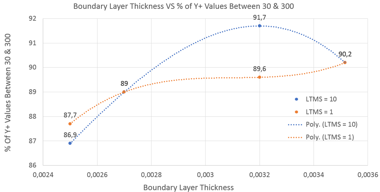
The second graph shows the Boundary Layer Thickness VS the percentage of Y+ values that landed between 30 and 300. This data also shows no trend between the different LTMS settings so further testing would be needed.
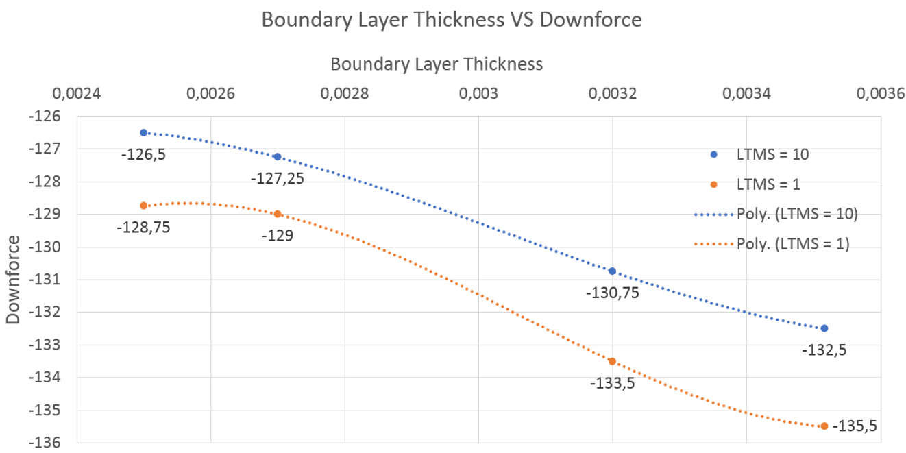
The next graph shows the Boundary Layer thickness results VS Downforce and then Drag. For the Downforce results, there is a clear trend. Downforce increased with an increasing boundary layer thickness and also with the lower LTMS setting of 1.
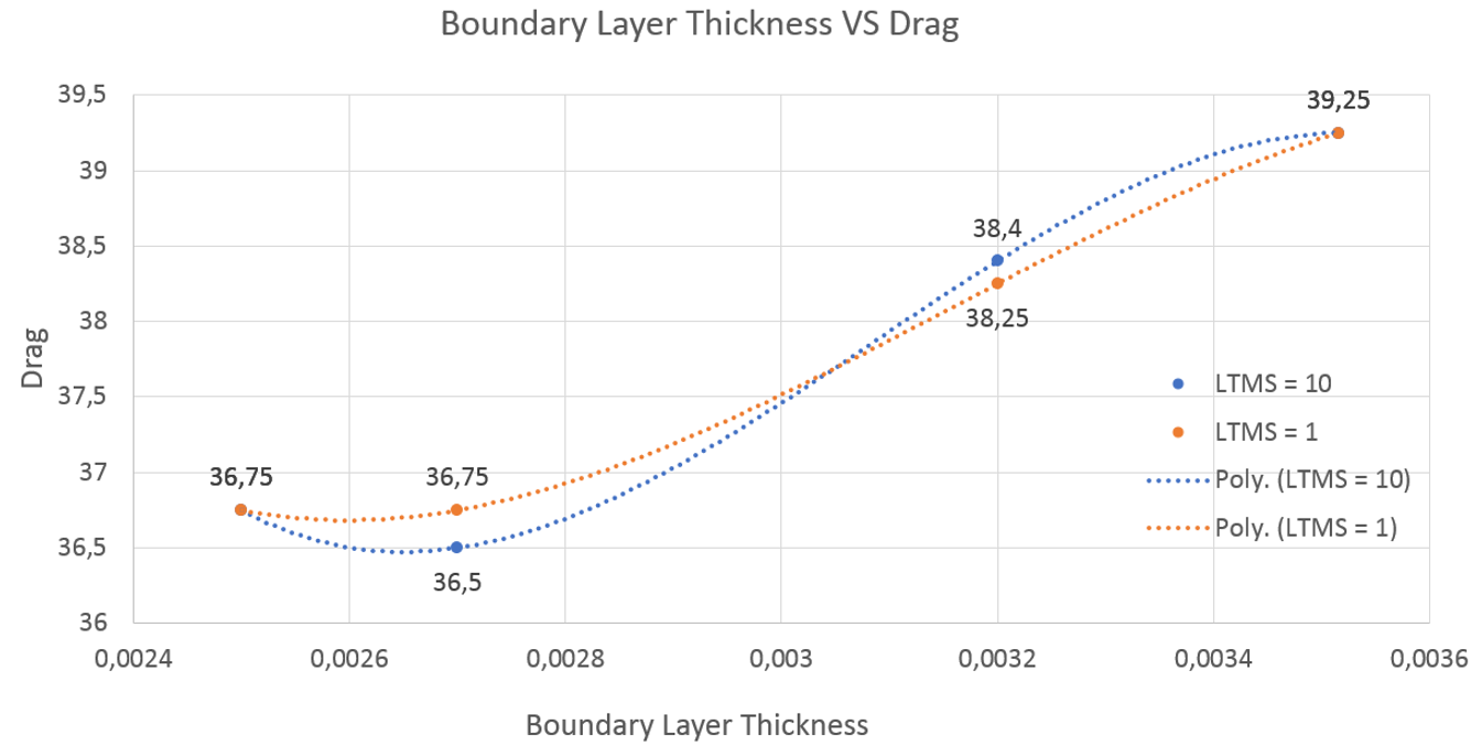
For Drag, the results are not so conclusive. The Thinner Boundary layer runs showed slightly more drag before transitioning to slightly less drag for the 0,0032m run. However, since the difference between results are so similar, it is difficult to verify a trend. For such close data points, it would again be necessary to run multiple simulations with a longer write interval and use a highly accurate data recording point from the force results graph. Therefore, I would conclude that the drag force results do not change based on the LTMS setting. However, just as with the Downforce results, Drag also shows an increase as the boundary layer thickness increases.
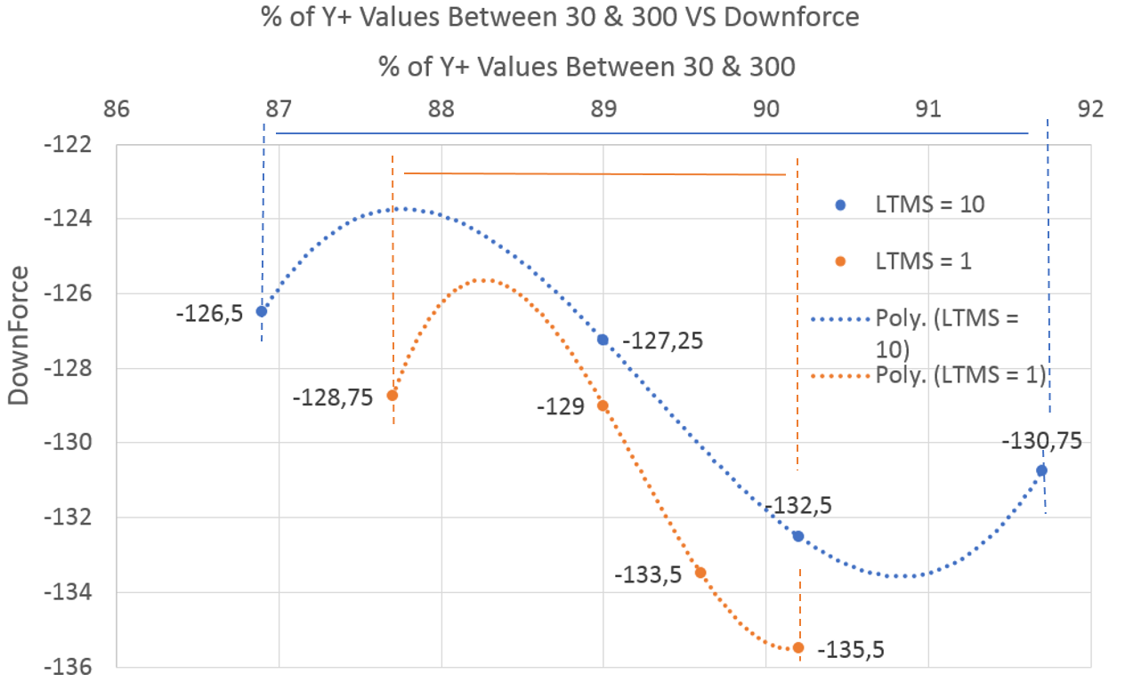
Finally, another interesting graph comes from the percentage of Y+ values between 30 and 300 VS the total Downforce results. The increase of total downforce using the LTMS setting of 1 has already been shown, however, with this comparison, the range of Y+ values can be better observed between the two tests. With a LTMS of 1, the range is much smaller (87,7 to 90,2) = a 2,5% difference compared with a LTMS of 10 which has a range of (86,9 to 91,7) = a 4,8% difference.
Another interesting occurrence is that for the LTMS 10 runs, the second to last and highest downforce result of -132,5N comes from the slightly lower Y+ percentage value of 90,2% in comparison to the last run with a downforce of -130,75N at 91,7%. In contrast, for the LTMS 1 runs, the trend of higher Y+ values between 30 & 300 resulted in a higher amount of downforce.
I apologize if these graphs are confusing, they are a bit for me as well. The point was to show two things. First, that comparing downforce results with a change in boundary layer thickness or Y+ values requires a lot of testing to achieve any kind of confirmed trend. Secondly, portraying the values in this way helped me understand the results a bit better. If the written descriptions are making things worse, just look at the nice colors and lines. In the end, CFD is all about pretty pictures, so accuracy doesn’t matter. 
Y+ Verification Test Summary
Through all this testing, I feel that there are a few areas where progress has been made. In my opinion, the highlights of the testing are as follows:
-
There is a clear advantage to using a low Layer Thickness Max Smoothing value, with 1 having good results. Despite its minimal improvement in total Y+ values, the reduction of meshing time and illegal cells is more than worth it. Plus, the meshing log shows an increase of layer thickness over many patches.
-
Inspecting the geometry for Y+ surface values is critical to understanding WHERE the Y+ values are out of range. If these areas do not drastically effect results, then they can be ignored.
-
Based on my testing, there is inconclusive evidence on a specific Boundary Layer cell size or Y+ value achieved that will be best under all conditions. Perhaps a comparison to lift and drag coefficients would have been more appropriate. In any case, having fully inflated boundary layers on the geometry is the most important.
Please let me know if any of my methodology is wrong. I dont want to spread misinformation due to a lack of experience or knowledge.
Dan