Here I have a solution with frictional contact for 1st order elements. For this I have already the results. But of course I would like to update the level of the simulation. Unfortunately until now somehow the model with 2nd order elements and frictional contacts just don’t wan to run.
Do you have any idea what should be corrected in the model (I think a setting is badly used by myself )?
I had a look at your project. There are certain things you can do to make it work.
In your first order case, you have swapped master and slave entities. This you can do here also.
You can delete the other elastic supports while just keeping one. For example, keep only Elastic 1 in your case. Since you have bonded contacts between all the nut and bolts, this elastic support will be enough for holding it.
Under Equation solverMUMPS, there is an option that says Stop if singular. Make it false. This will enable to run your simulation further even if there is singularity. And this singularity is mostly due to rigid body motion and if the elastic support is too low that it can’t solve this in very first iteration.
If result accuracy isn’t important in the first trials, you can increase your relative error tolerance to 0.001 to attain fast convergence.
Switch to Auto timestepping with Initial timstep length of 0.1. Using Manual will not allow the solver to cut the timestep in case of divergence which will for sure happen at start. Furthermore, use 8 core machine and 2 cores for computation in order to avoid memory problems.
Delete cauchy stress solution field under Result Control if you don’t need it. This will save you some time.
I hope this helps. If you still face some problem, feel free to ask.
I tried all of the suggested changes. The run was not successfull and the log file contains no information at all. Do you have any further idea? Thanks a lot for your help!
Hi @ahmedhussain18, this is good news! I’ve been wanting to use this functionality for a long time and until now I did not think it was possible. I think the setting I was missing was “Stop if singular = FALSE”. I’ll give it a try.
Hey @BenLewis! well this is not exactly the case. In my other several cases, even putting it to false didn’t help. I think this case is quite simple due to which it worked. But if there is large sliding involved, it is HARD to converge!!
As Ahmad wrote, the simulation was really running. The only difference what I recognized between Ahmeds and my settings was the Penalty coefficient. By Ahmed it was 100000000000, while by me it was 1000000000000. I changed it and the run was made perfectly and I have results. Thanks a lot for this amazing support work of the whole SimScale team and especial for @ahmedhussain18!
Yet I have further questions by the postprocessing:
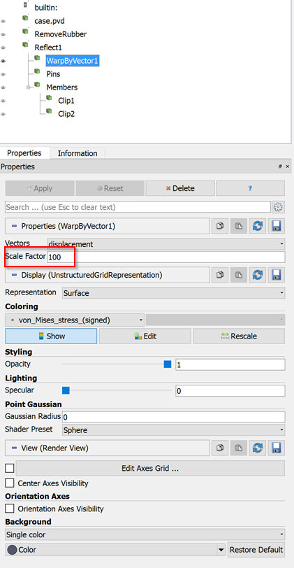
How can I create plots in deformed state and how can I set the value of the deformation scale (1x, 2x, 10x, etc…)
What are the units of the results? von Mises; displacement; nodal force;
Do you have a documentation where I can read for example what do you mean under “total non linear strain”?
Do you have an idea how could I check whether the 0.1 mm fictitious clearance between the physical contacts really tok place? Until now I failed to do this anyhow I tried.
You can use the “WarpByVector” filter in the online post processor and in ParaView. In ParaView you will find it under Filters > Alphabetical > Warp By Vector. You will need to use the displacement vector for scaling and enter a scaling factor for the magnitude of the deformation.
SimScale uses SI units (for simulation set up and results):
mass: kg
length: m
time: s
force: N
stress: Pa
energy: J
I not aware of any documentation for this. @ahmedhussain18 might be able to help you out here. My understanding is that strain can be either linear (elastic) or non-linear (plastic). You can view just the plastic component of strain with total non-linear strain or just the elastic component of strain with total linear strain. Oy you can view the combined elastic and plastic strain with total strain.
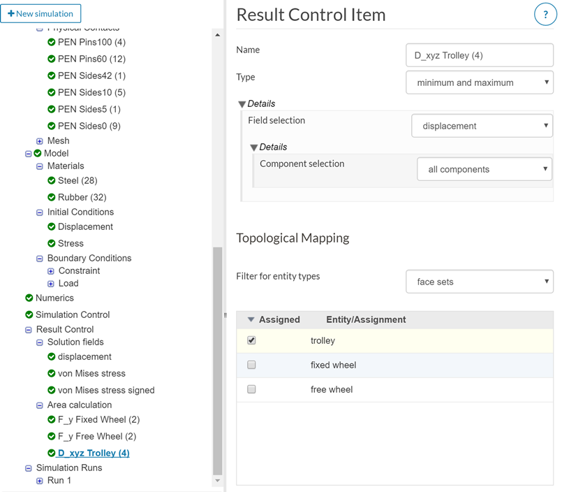
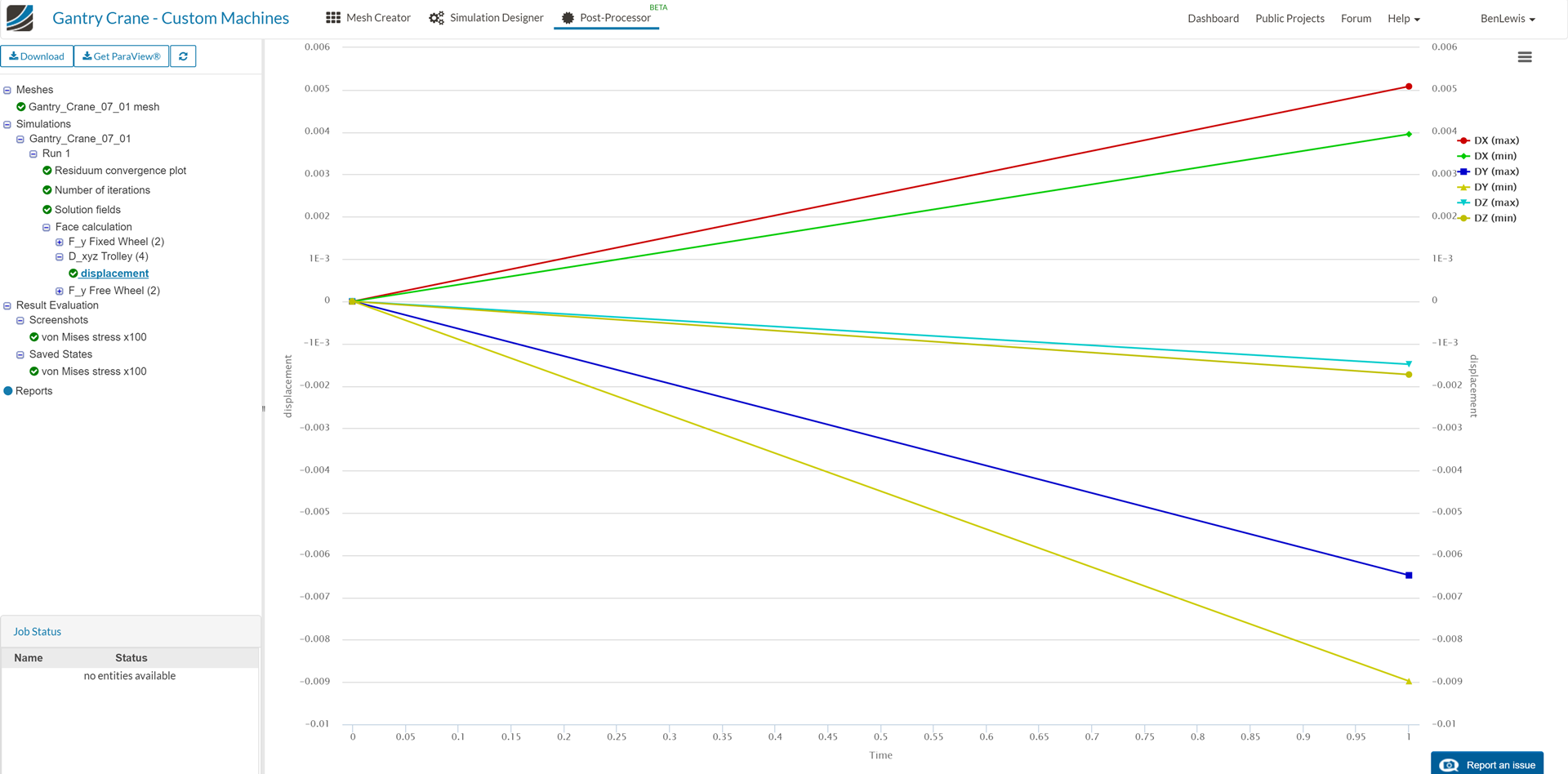
You can do this by plotting displacement in the post processor or by applying a “Results Control” measure in the simulation designer. Below is an example of a definition that measures displacement in the X, Y and Z directions.
@potyka_csaba! Regarding documentation of solution fields we are progressing towards them. As there are many things beforehand to improve which are quite important than solution fields. @BenLewis already explained it pretty well, other then that you can always search on web about these solution fields as they are fairly similar to other simulation softwares.
Hello @potyka_csaba@BenLewis@ahmedhussain18,
maybe I can explain the meaning of the most important stress and strain result fields.
First, lets clear the notation:
u_{i,j} = \frac{\partial u_i}{\partial j}
and
u_{k,i}u_{k,j} = \sum_{k=1}^{3} u_{k,i}u_{k,j}
For the stresses we have:
Cauchy stress tensor: The most basic and most important stress measure. Directly from the Cauchy postulate:
von Mises stress (signed) : The signed von Mises stress has the same absolute value as the normal von Mises stress, but it has a sign that is determined by the sign oh the hydrostatic stress to distinguish between compression and tension .
\sigma_{vs} = sign(tr(\sigma))\sigma_v
Tresca stress : Scalar stress criteria by Tresca
\sigma_{tr} = \sigma_{I}-\sigma_{III}
For the strains we have:
total linear strain: This is often also referred to as engineering strain, it’s a simple linearized strain measure derived from the Cauchy stresses without second order terms
\epsilon_{ij} = \frac{1}{2} (u_{i,j}+u_{j,i})
total nonlinear strain: This is originally called Green-Lagrange strain
P.S.: @ahmedhussain18 Meanwhile I think I found the problem; my contact settings are too “soft” and due to the large penetration I don’t get those results what I would expect. That is why I asked what kind of units are shown in the post processing because I was not able to find out why I see what I see.
I just try to increase the penalty coefficient to see whether the results will be better.
@potyka_csaba! Yes, indeed penetration is always a problem. I just did these preliminary simulations. One can for sure do it with higher penalty stiffness which in turn will take more time to converge. But of coarse to get better results, you have to take this thing in consideration
Please give me some info about the element formulations in SimScale for Code-Aster advanced static problems!
What is the element correspondence (1st order and the 2nd order) between SimScale and Code-Aster?
The contact formulation is discrete or continuous corresponding to Code-Aster?
Please give me some advice how could I get run the model “2ndelAugmLagfrict” in my project: https://www.simscale.com/workbench?publiclink=6a77111a-5e14-4abb-b4b1-f27f94976881
(NOTE: for 1st order elements it is fine even with friction, but the 2nd order elements seem to be not that well conditioned for the contact algorithm, nevertheless it should work without any problem based on the Code-Aster documentation…)
Your help is extremely priciated
Thanks in advance,
Csaba
Hello @potyka_csaba,
let’s first answer the easy questions:
The element type depends not on the mesh order, there is an additional setting as a child of the assigned mesh in your simulation that is called Element Technology. There you can choose the “finite” element type. For the 3D elements, you currently have the choice between standard (equals 3D in Code-Aster) and reduced integration (equals 3D_SI in Code_Aster). There are more to come, especially incompressible elements.
We are using only the continuous formulation, since this is the most complete and robust one, especially for friction.
As a side note, if you have a look at the beginning of the Solver log, there you find the complete set of Code_Aster commands that is used for the run. You can review each setting that you are interested in (if you understand the Code-Aster command file syntax).
I did not yet have a look at the project you mentioned, but generally there can arise problems with contact on second order elements. It’s mentioned in the Code-Aster documentation, for example in the document Note of use of the contact: In formulation continues, for meshes of edge curves, the use of elements QUAD8 or TRIA6 can involve violations of the model of contact: this last is checked on average. One then observes clearances slightly positive or slightly negative in the presence of contact, which can disturb the results close to the contact zone or computations in recovery with initial state. For this reason it is advised to use elements HEXA27or PENTA18 (with sides QUAD9) or many linear elements.
Currently we don’t have the support for HEXA27 or PENTA18 elements.
I’ll have a look at you sim to see if we can get it to run nevertheless.
Best,
Richard
What do you mean by continuous formulation? This is also something that is not discussed in the documentation. From the textbook, types of implementations for contact include:
Node-to-node
Node-to-segment
Integration point-to-segment
Segment-to-segment
When you say continuous, do you mean segment-to-segment?
Penalty vs. Augmented Lagrange
Additionally, the documentation says that the “Lagrangian” approach is not stable compared to penalty. But the UI calls is “Augmented Lagrange”. So I am a bit confused if the implemented method is “Lagrange multiplier” or “Augmented Lagrange multiplier”.
From what I understand from my own contact implementations is
Large penalty factors can lead to ill-conditioning of the stiffness matrix. As penalty parameter tends to infinity, it leads to an exact solution. Else penalty method should have small (though negligible) interpenetration.
Lagrange multiplier method is exact but adds more equations. Additionally, it can lead to oscillatory behavior at the transition zone.
Augmented Lagrange multiplier method combines the good qualities of both the above worlds. Computationally, it definitely leads to a bigger system of equations. But that is a small price to pay for accuracy & robustness.
So I am wondering why it would be any less stable than the penalty method as mentioned in the documentation?
Mortar formulation?
Also what if you have non-matching meshes on the two sides. Is it using a mortar method? If not, how are these handled?
Hello @ajaybharish,
good questions! I’ll try to answer them one-by-one:
The wording continuous formulation is a wording that comes from the underlying tool that we use for the advanced analysis types (Code_Aster) and rather a distinction to the other available formulation, the discrete formulation. The discrete formulation is called that way, since it uses already discretized fields such as displacement and nodal forces in the contact equations. It’s available with a node-to-segment and a node-to-segment pairing.
We decided to only include the continuous formulation since it is the more generic one and better usable with friction. The continuous formulation uses a node-to-segment pairing.
The wording in the documentation is indeed not explicit enough. In this case the correct naming is Stabilized Lagrangian Method, but it is equivalent to the Augmented Lagrangian Method, for details you can have a look at this phd thesis by Ayaovi Dzifa Kudawoo.
This is partly related to the general nature of the Penalty Method and also the current implementation of the Augmented Lagrangian Method.
Generally the source of (almost) all difficulties when dealing with physical contact is the high nonlinearity of the contact conditions, they are not only nonlinear, but non-differentiable and discontinuous. Since the Penalty Method itself smoothens the strong contact assumptions by allowing a certain amount of penetration, reduces the numerical difficulties. Of course, the method itself introduces another source for numerical problems as you stated, but with a reasonable starting value for the penalty factor most contact analyses will at least give an initial result. This can be then used as a starting point to further refine your setup and finally reach converged results.
The Augmented Lagrangien Method can have problems with over-constrained simulation setups, for example when symmetry and frictional contact constrain the same DOF. This might partially be related to the current implementation, but experience has shown that in those cases switching to a penalty contact often solves the problem.
I am not sure how far you want me to go with an answer to this one. The contact surfaces are generally never matching. The current implementation does not use a mortar method. You can find all details of its implementation in this document of the official Code_Aster documentation.
As a side note: Recently there was an improved contact method for non-matching meshes implemented into Code-Aster that is going to be integrated into SimScale as soon as it’s stable. Details can be found in this paper.
If you have any additional questions, I’m happy to help.
Best,
Richard