This post is a continuation of Aerospace Workshop 2 Session-1 Homework and it contains the tutorial to setup the simulation for Aircraft wing/blended winglet.
Simulation Setup
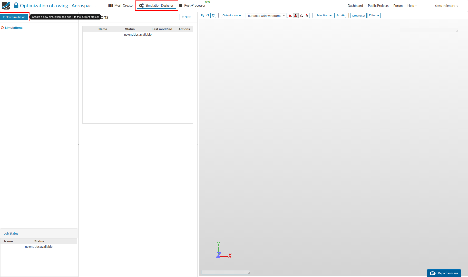
- For setting up the simulation switch to the Simulation Designer tab and select New simulation.
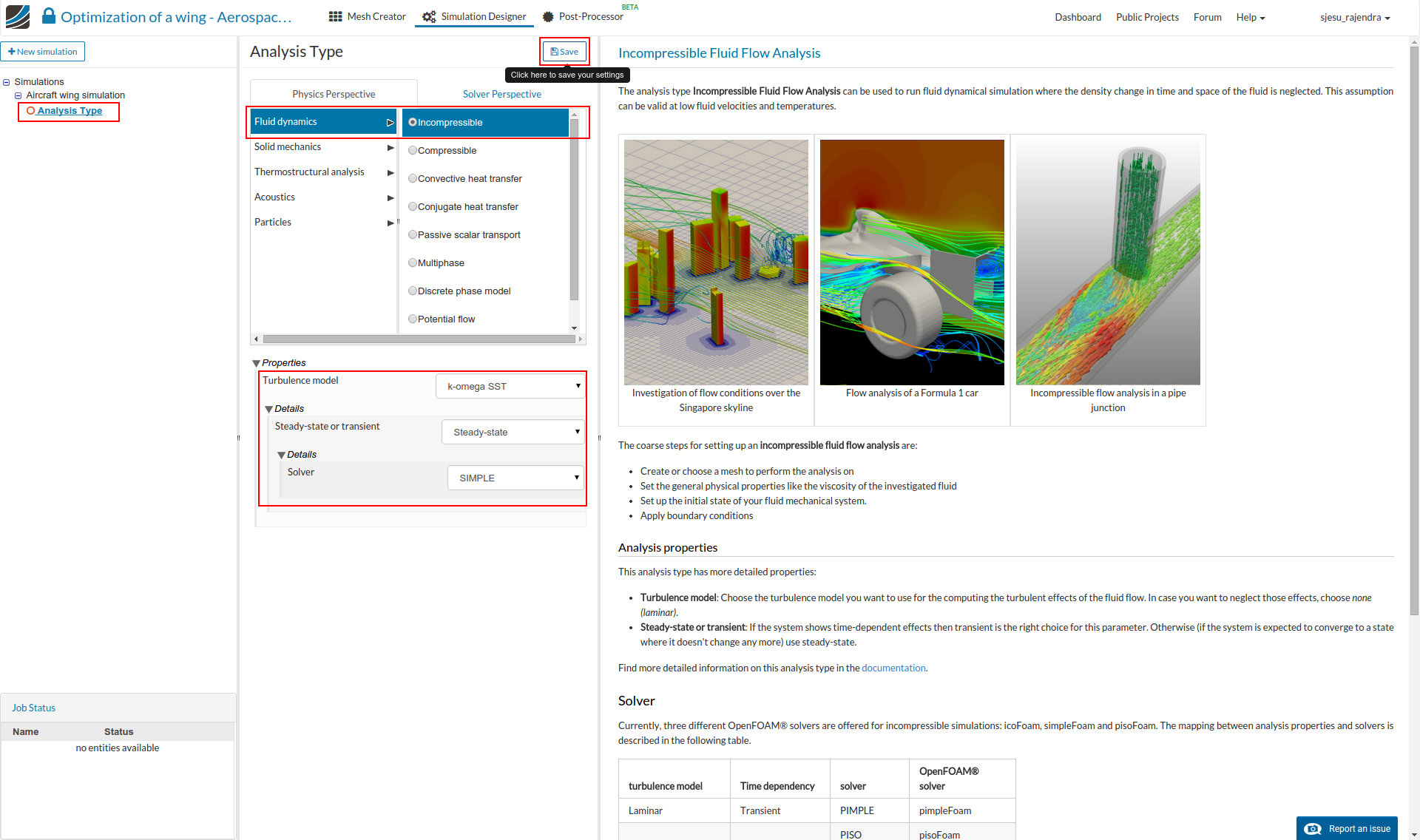
- Select the analysis type: Incompressible under Fluid dynamics.
- Select k-omega SST as the turbulence model and Steady-state type and click Save button.
- The flow is assumed to be Inompressible due to velocities lesser than Mach 0.3. Choosing Steady-State option means that we will simulate the Time-Independent solution.
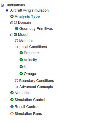
- After saving, the simulation tree now looks as shown below. Here the Tree Entries in Red must be completed.
Domain selection
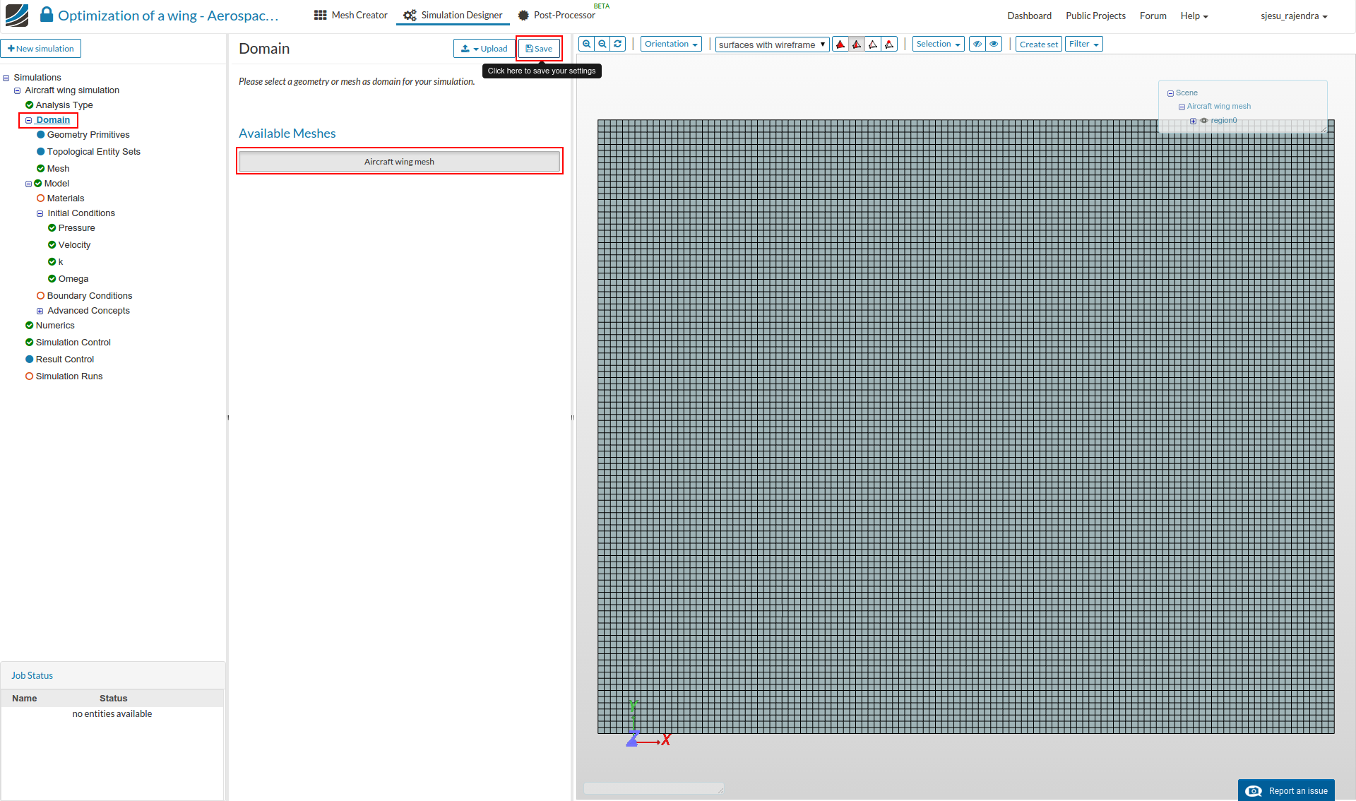
- Click ‘Domain’ from the tree and select the mesh created from the previous task. Click the Save button. The mesh will then automatically load in the viewer.
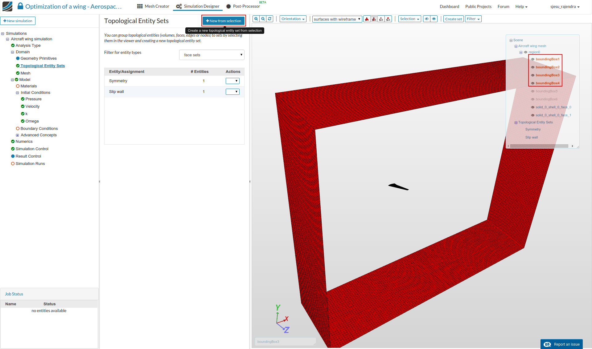
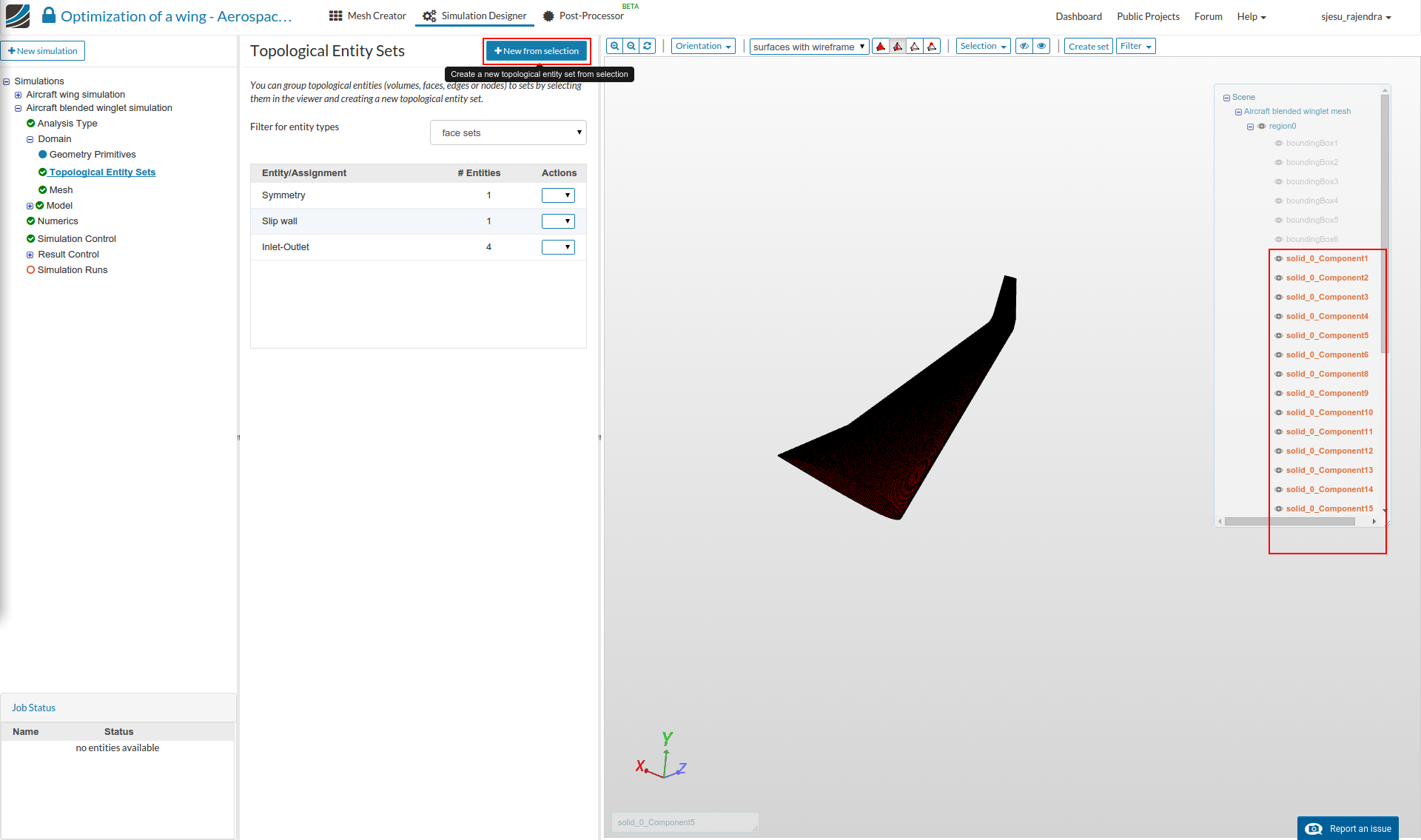
Create Topological Entity Sets
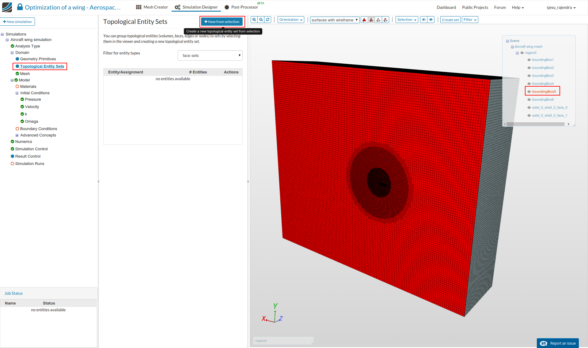
- Click on the tree entry ‘Topological Entity Sets’. The order of choosing the sets is based on ease of selection.
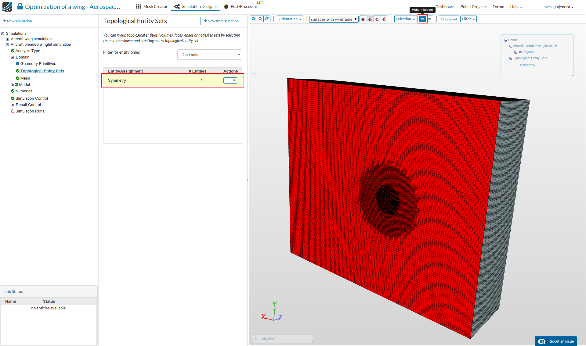
Symmetry:
- To create the first set, click the shown surface (boundingBox5) and click on the ‘New from selection’ button to create a set named ‘Symmetry’.
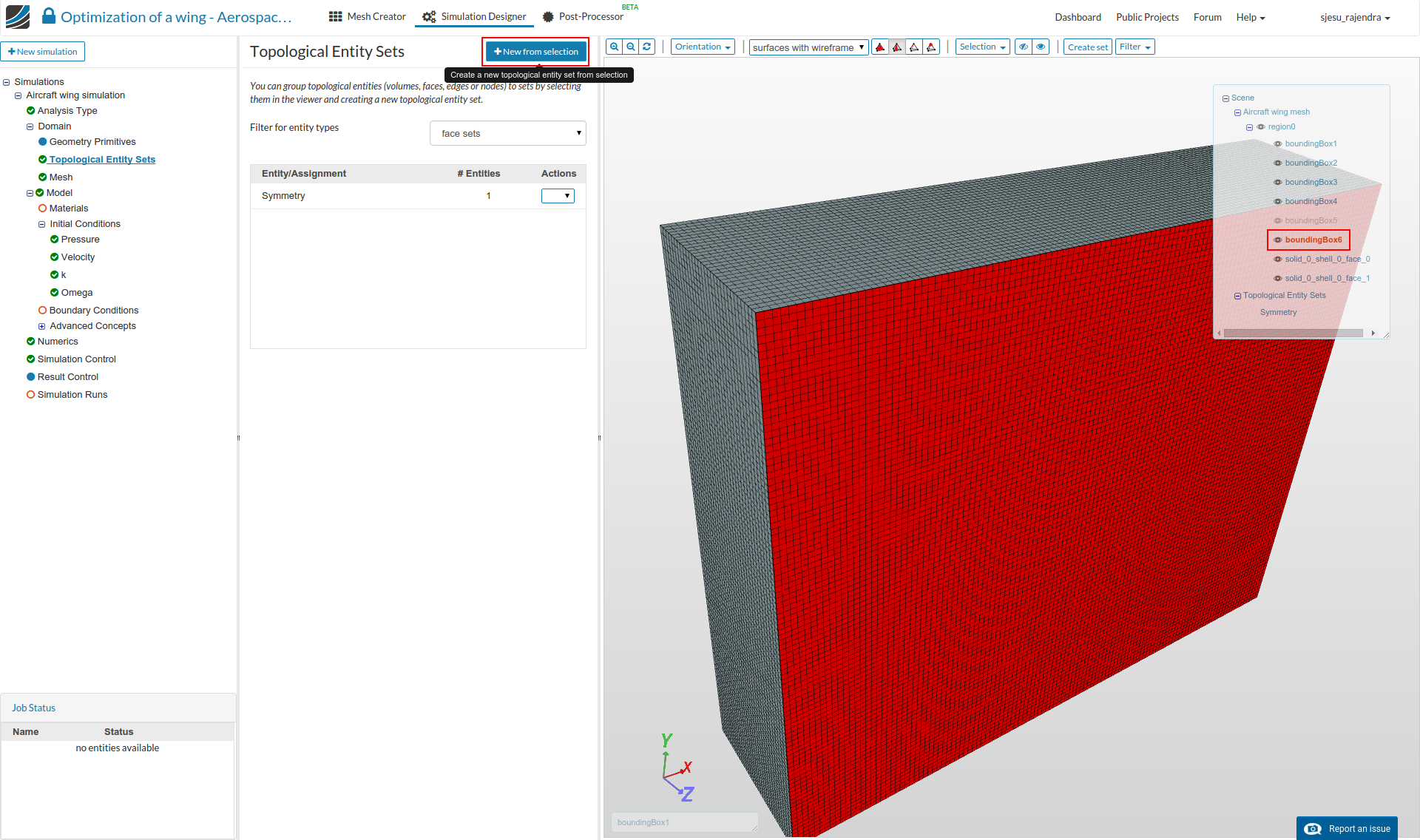
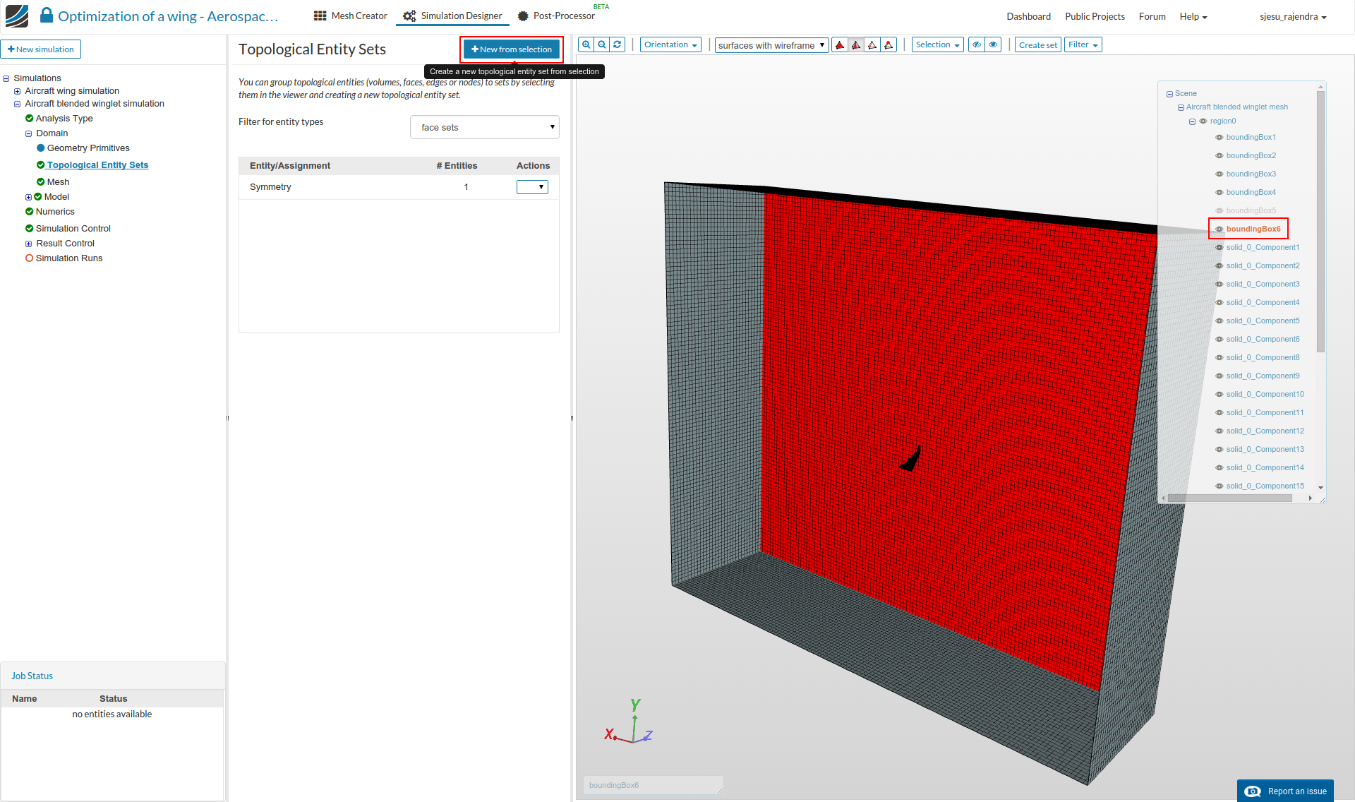
Slip wall:
- Similarly, select the shown surface (boundingBox6) and create a new set named ‘Slip wall’.
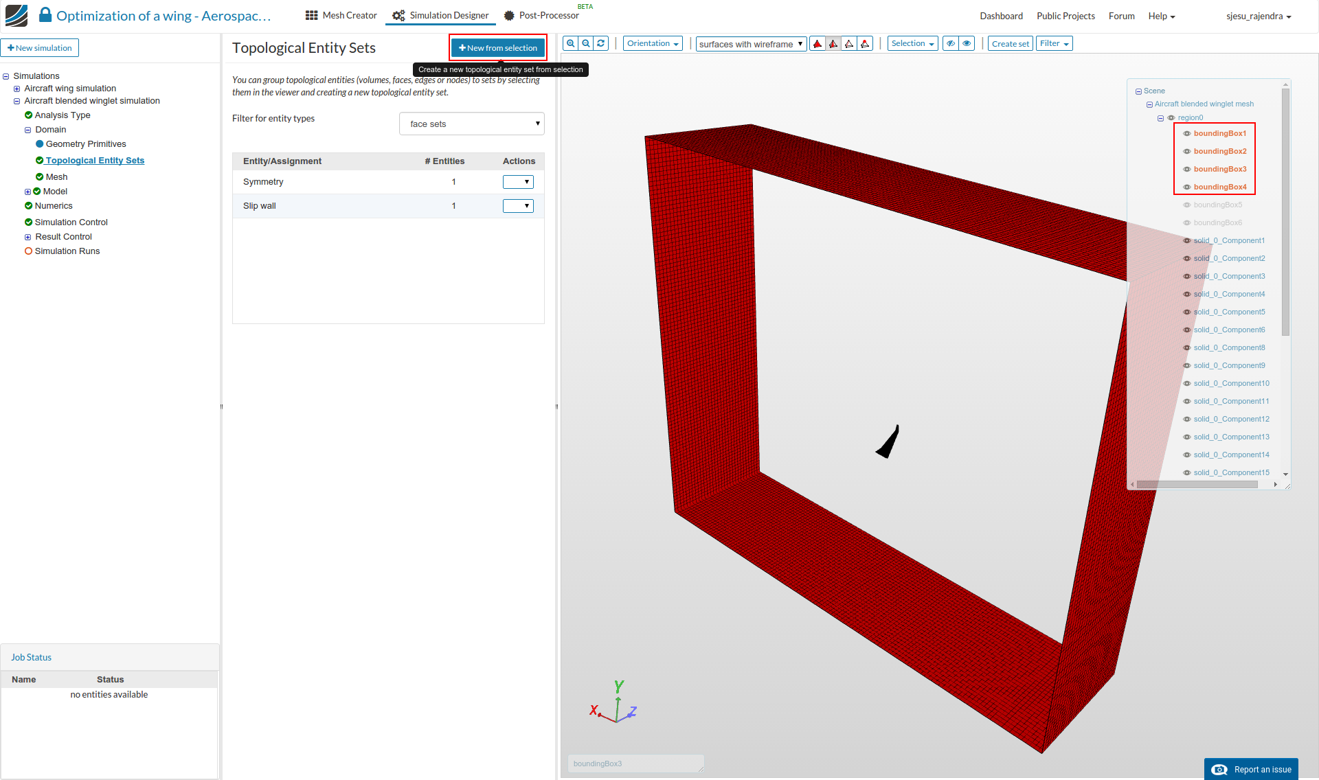
Inlet-Outlet:
- The faces shown below (boundingBox1, boundingBox2, boundingBox3 and boundingBox4) are selected for defining the ‘Inlet-Outlet’ condition
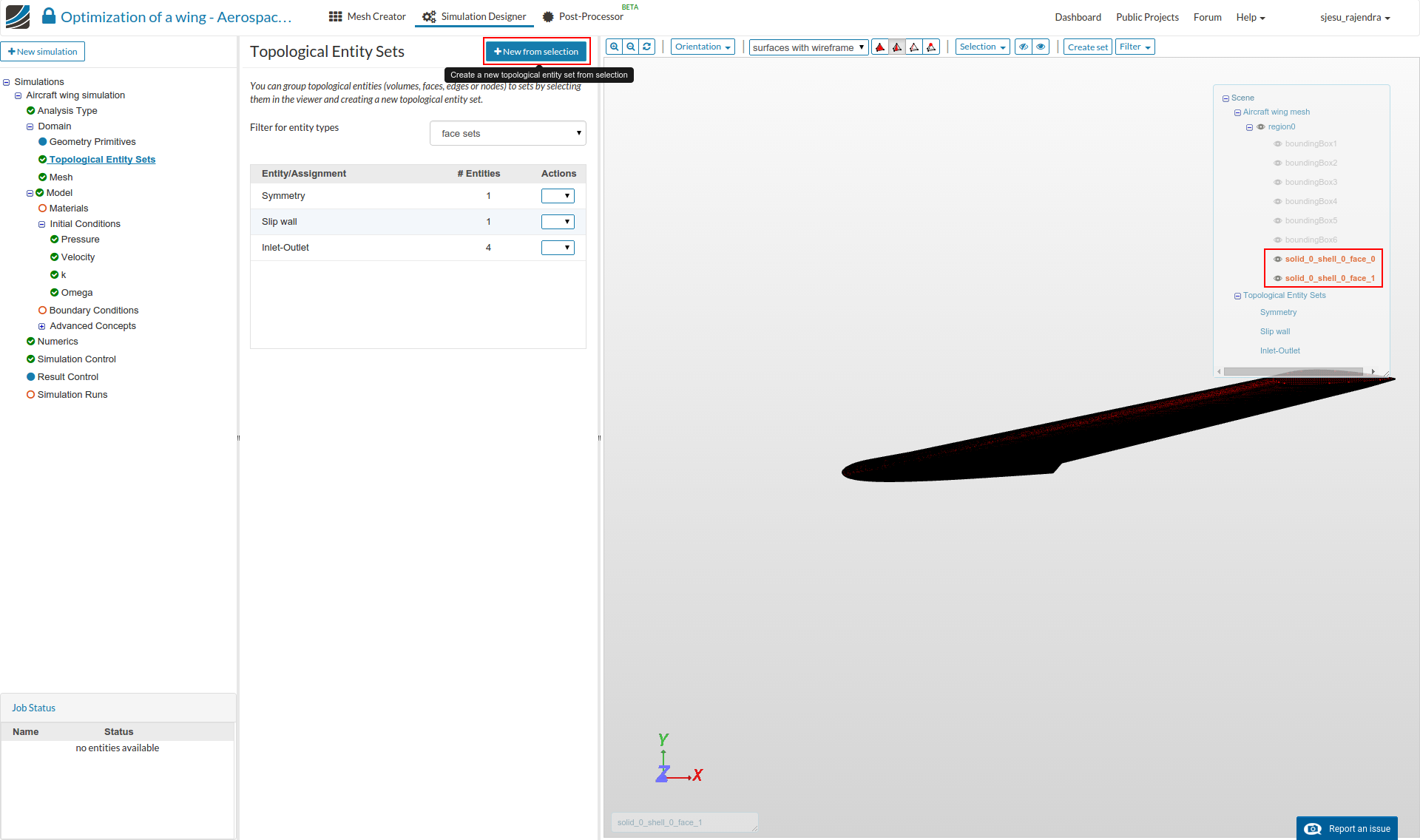
Wing:
- The Wing surfaces (solid_0_shell_0_face_0 and solid_0_shell_0_face_1) are selected and named.
Select Fluid Material
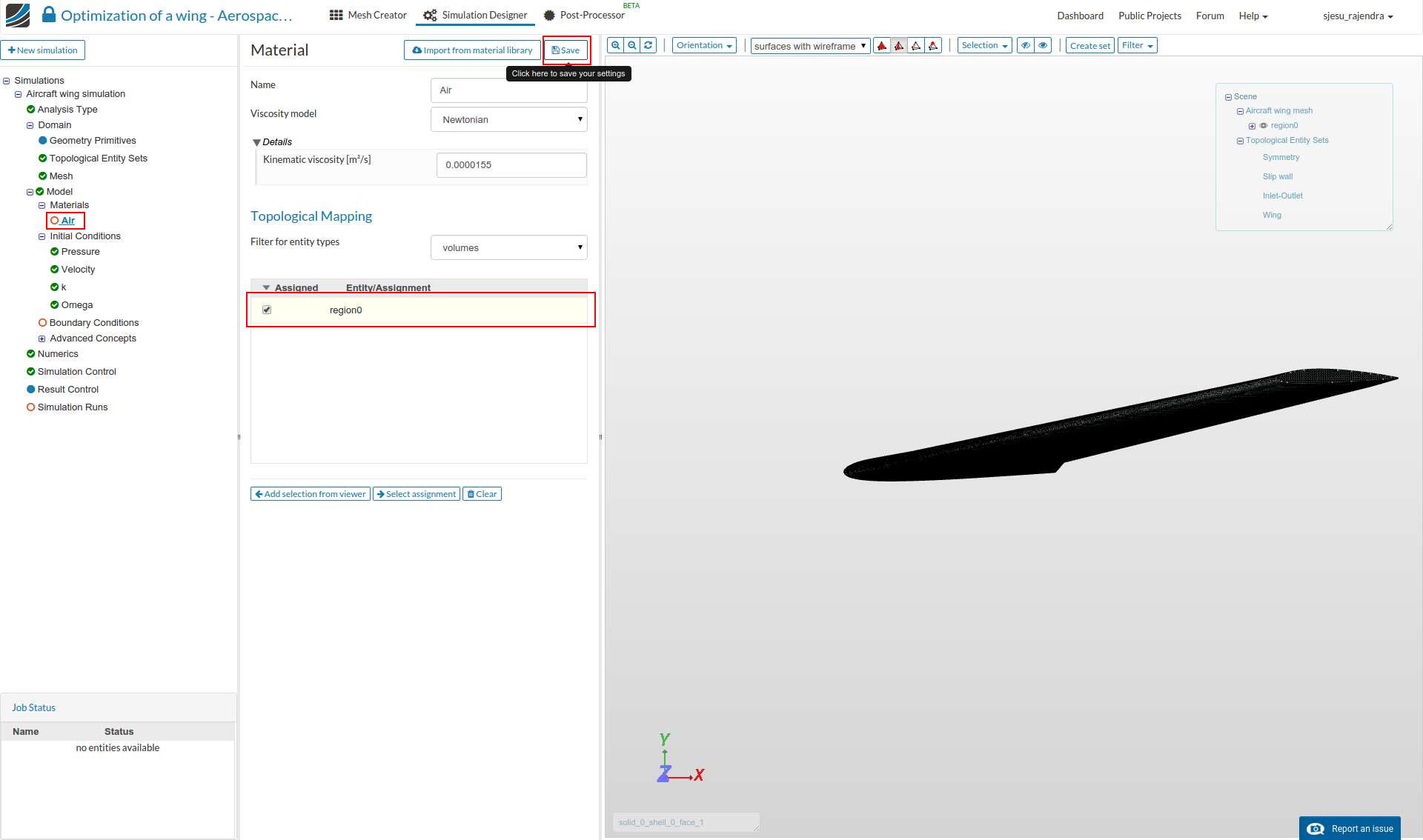
- Select ‘Material’ from the sub-tree and click New.
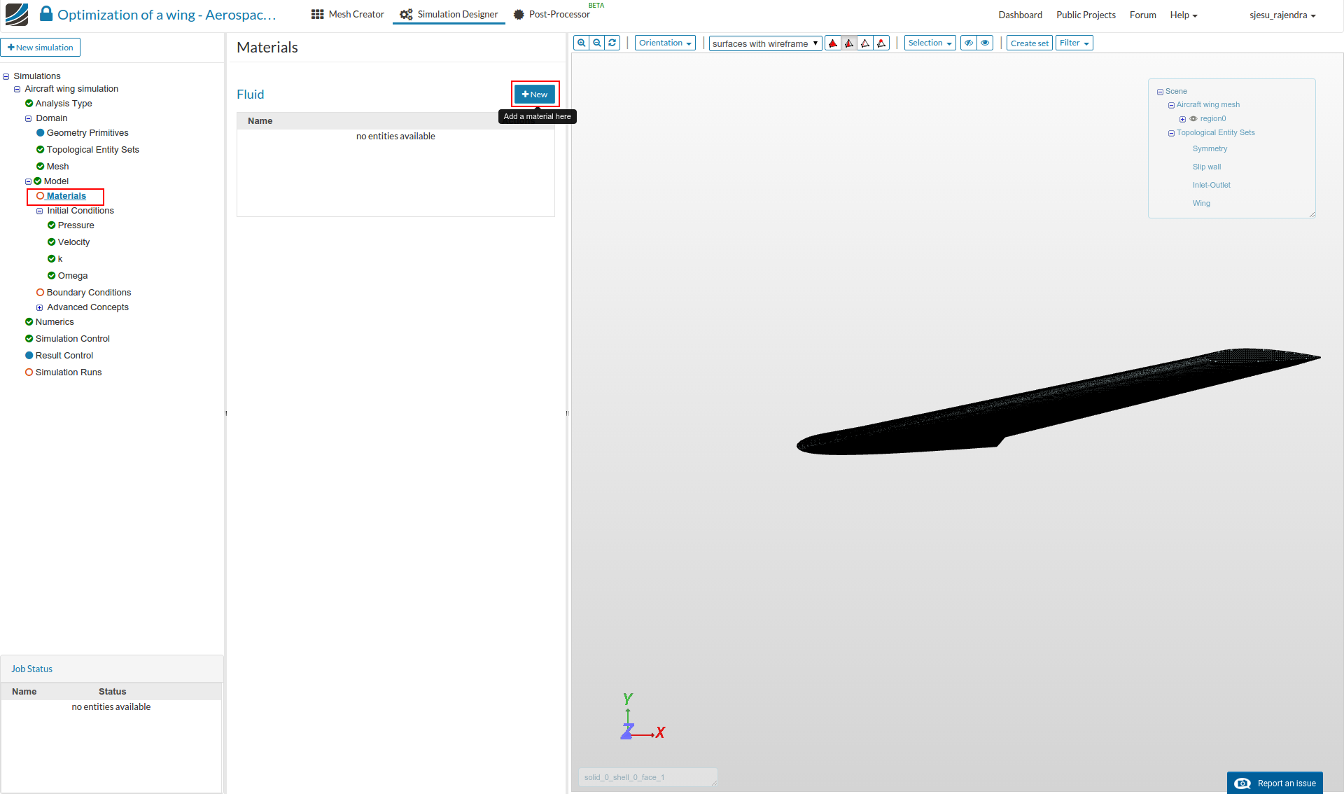
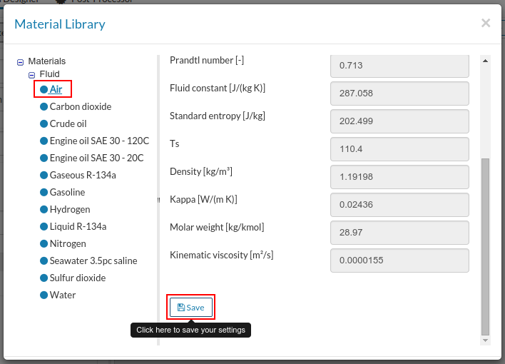
- Select Import from material library in the top of the pane.
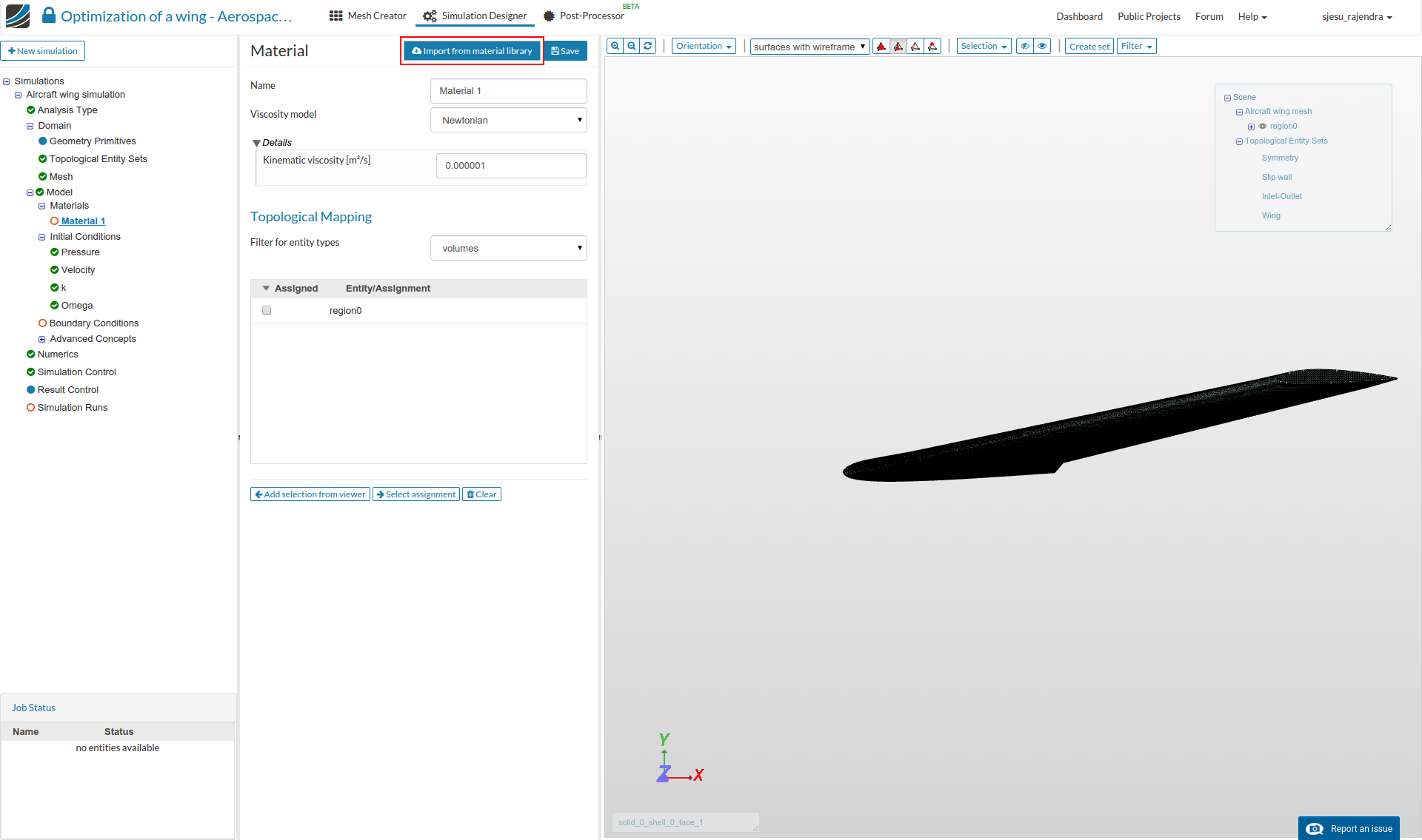
- Click Air and select the Save button.
- Select region0 from Topological Mapping and click the Save button.
Initial Conditions
- The following values are to be defined for initial conditions.
Pressure:
- Enter the pressure value 100000 [m2/s2].

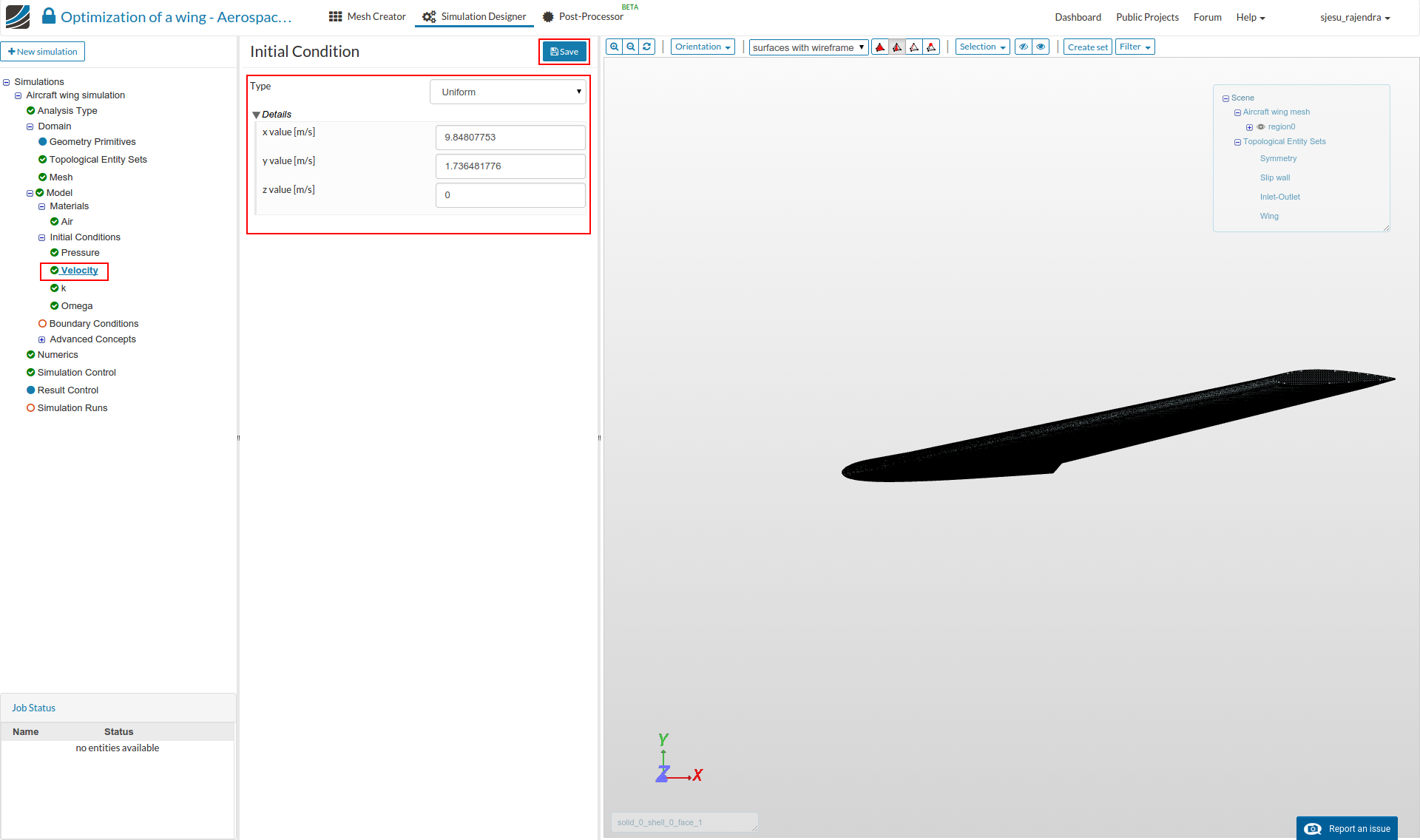
Velocity:
- Enter the velocity values 9.84807753 [m/s], 1.736481776 [m/s] and 0 [m/s] in x, y and z directions respectively.
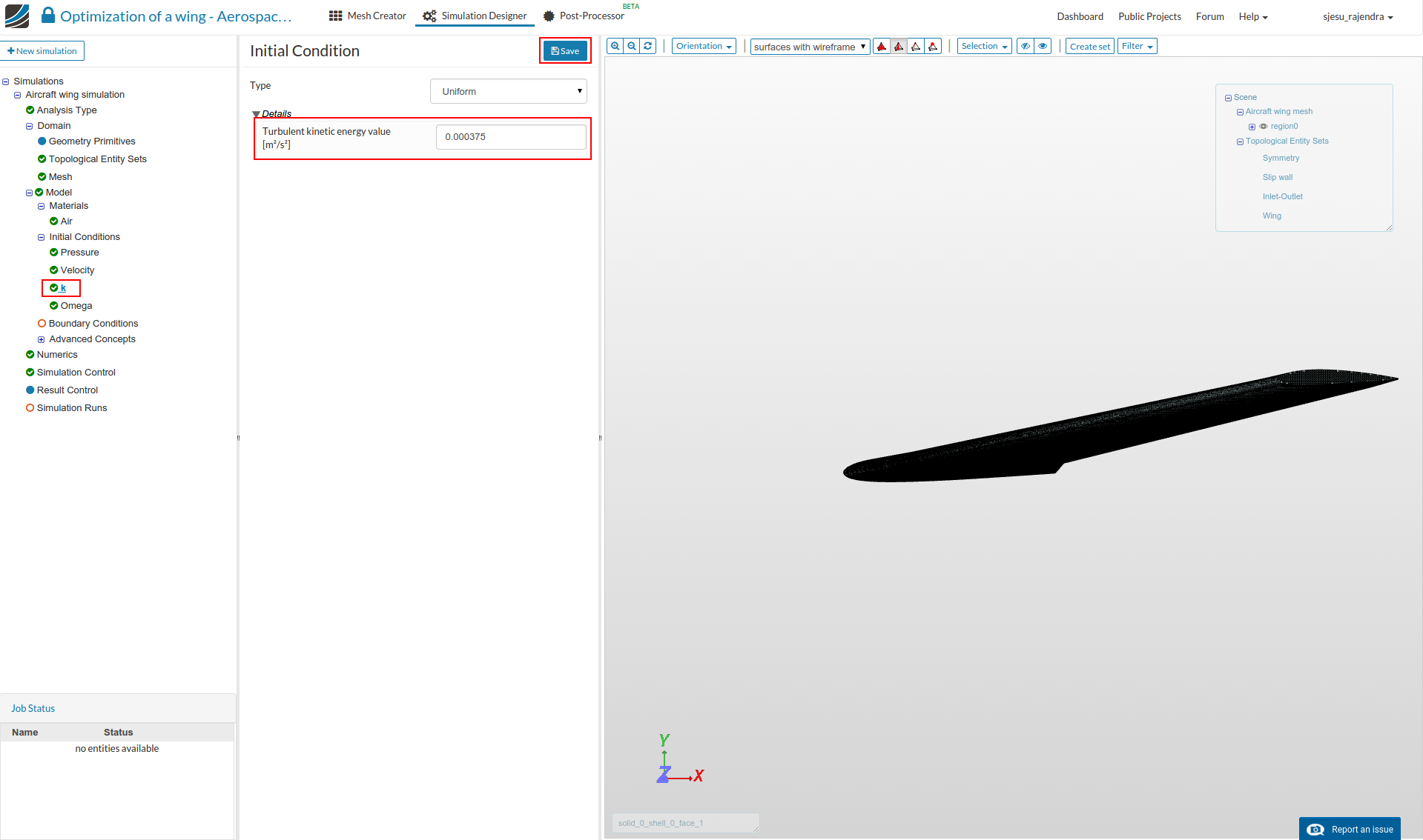
Turbulent kinetic energy:
- Enter the k value 0.000375.
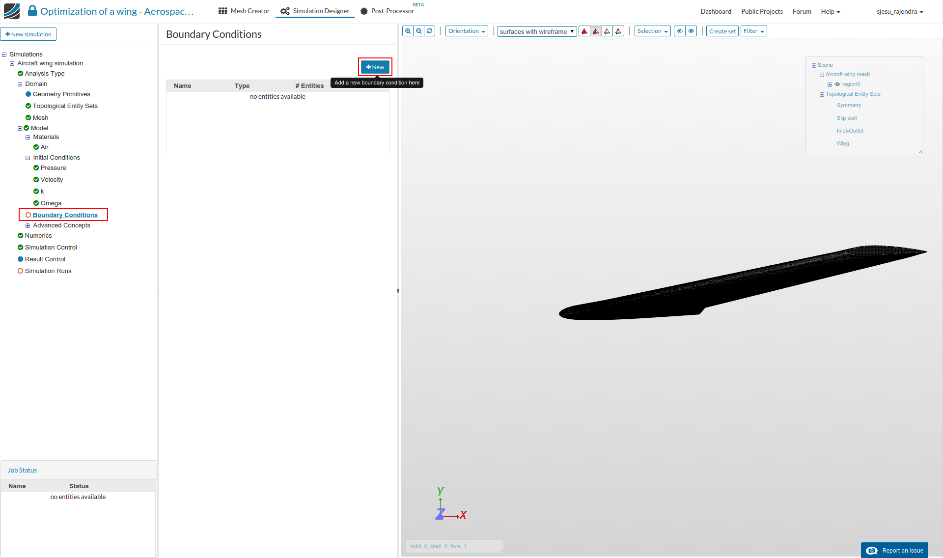
Boundary Conditions
The boundary conditions define the flow variables at the boundary surfaces.
- Click on ‘Boundary condition’ and select New.
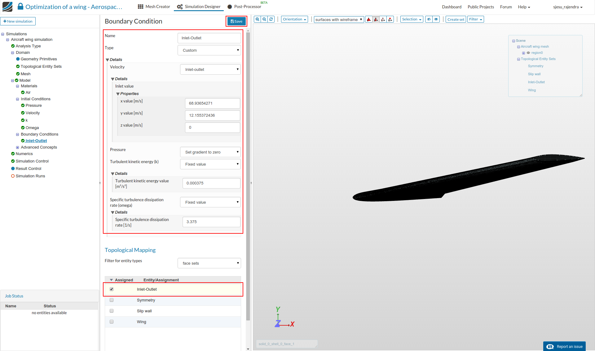
Inlet-Outlet:
- Enter the Custom boundary condition with a x, y and z-direction velocities of 68.93654271, 12.155372436 and 0 m/s respectively, and pressure set to Zero gradient. * Select the Inlet-Outlet entity and click Save option.
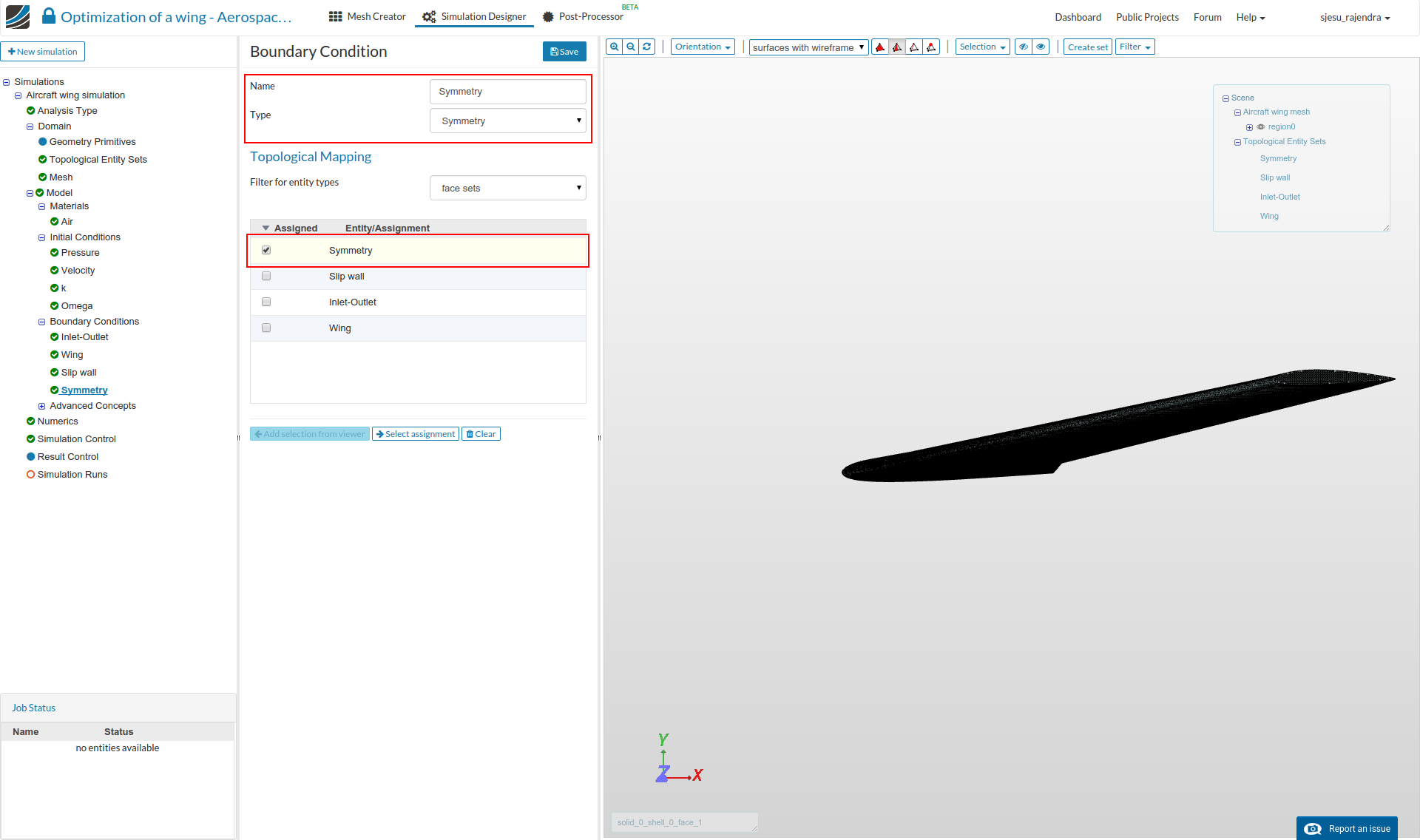
Symmetry:
- Next we will create the symmetry condition.
- Select a Symmetry boundary condition, select the symmetry entity and click Save option.
Slip wall:
- Create a boundary condition named Slip wall with Type Wall and velocity type Slip.
- Select the Slip wall entities and click Save option.

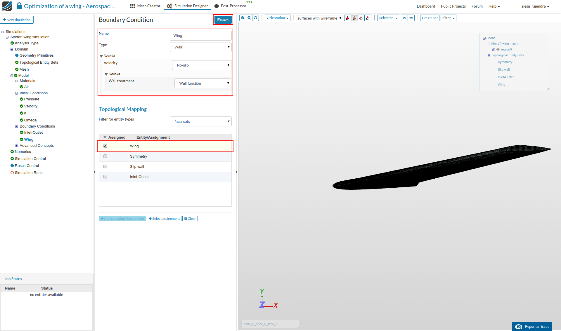
Wing:
- The remaining boundary definition is for the Wing.
- Create a New boundary condition of type “Wall” and velocity type with No-slip.
- Select the Wing entity and click Save .
Numerics
-
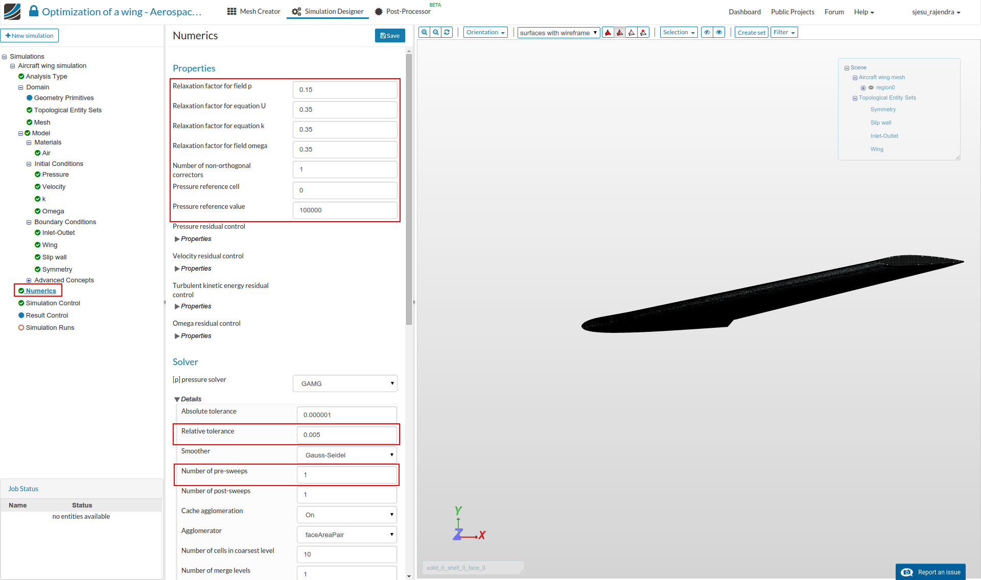
Select ‘Numerics’ from the sub-tree and enter the following values. This enhances the solver to get the appropriate results.
-
Set the relaxation factors to:
p : 0.15
U : 0.35
k : 0.35
Omega : 0.35
Number of non-orthogonal correctors : 1
Pressure reference value : 100000
- The relative tolerances for GAMG pressure solver is changed to 0.005
- Number of pre-sweeps 1
-
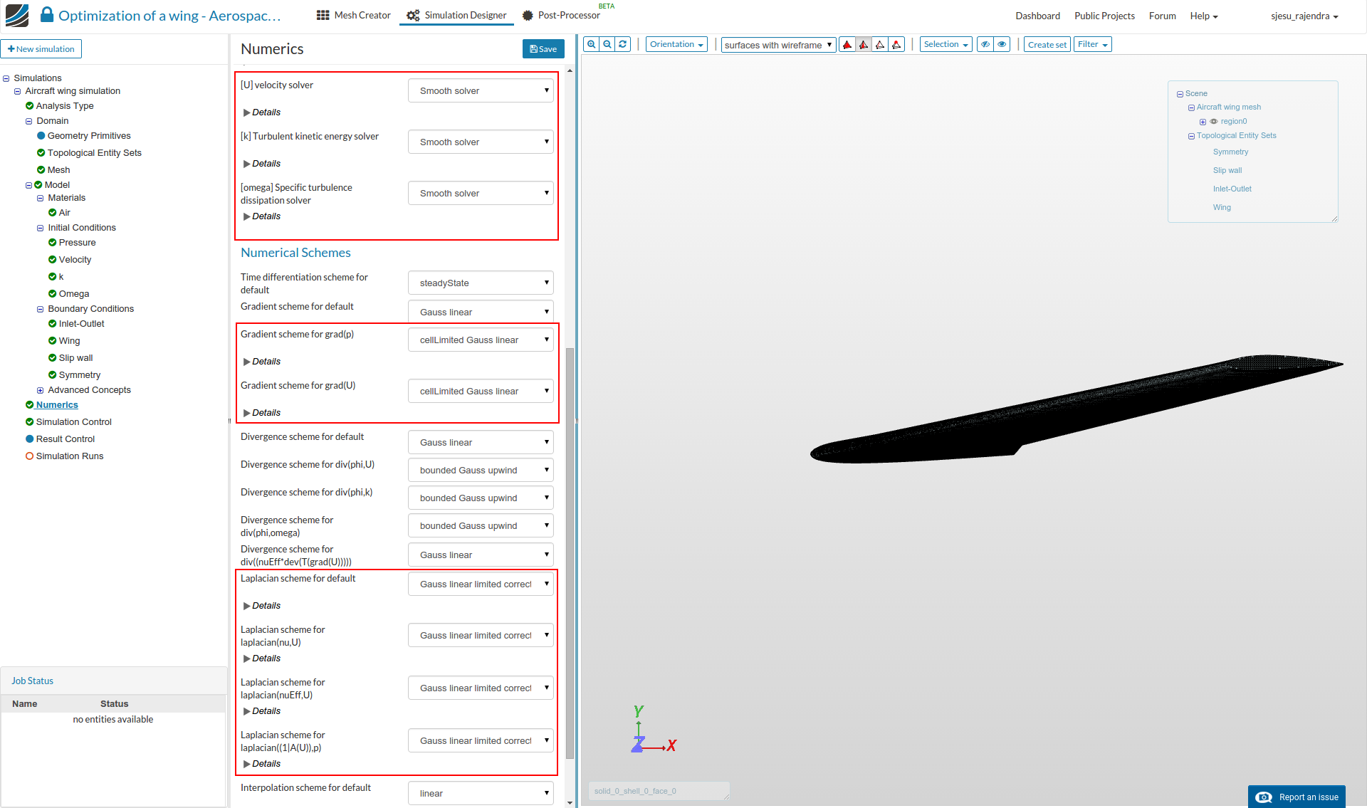
The velocity, turbulent kinetic energy and specific turbulence dissipation solvers are changed to Smooth solver with default settings.
-
The gradient schemes for pressure and velocity are changed to cellLimited Gauss linear type.
-
All the Laplacian schemes are set to Gauss linear limited corrected.
-
Set the divergence schemes to bounded Gauss upwind.
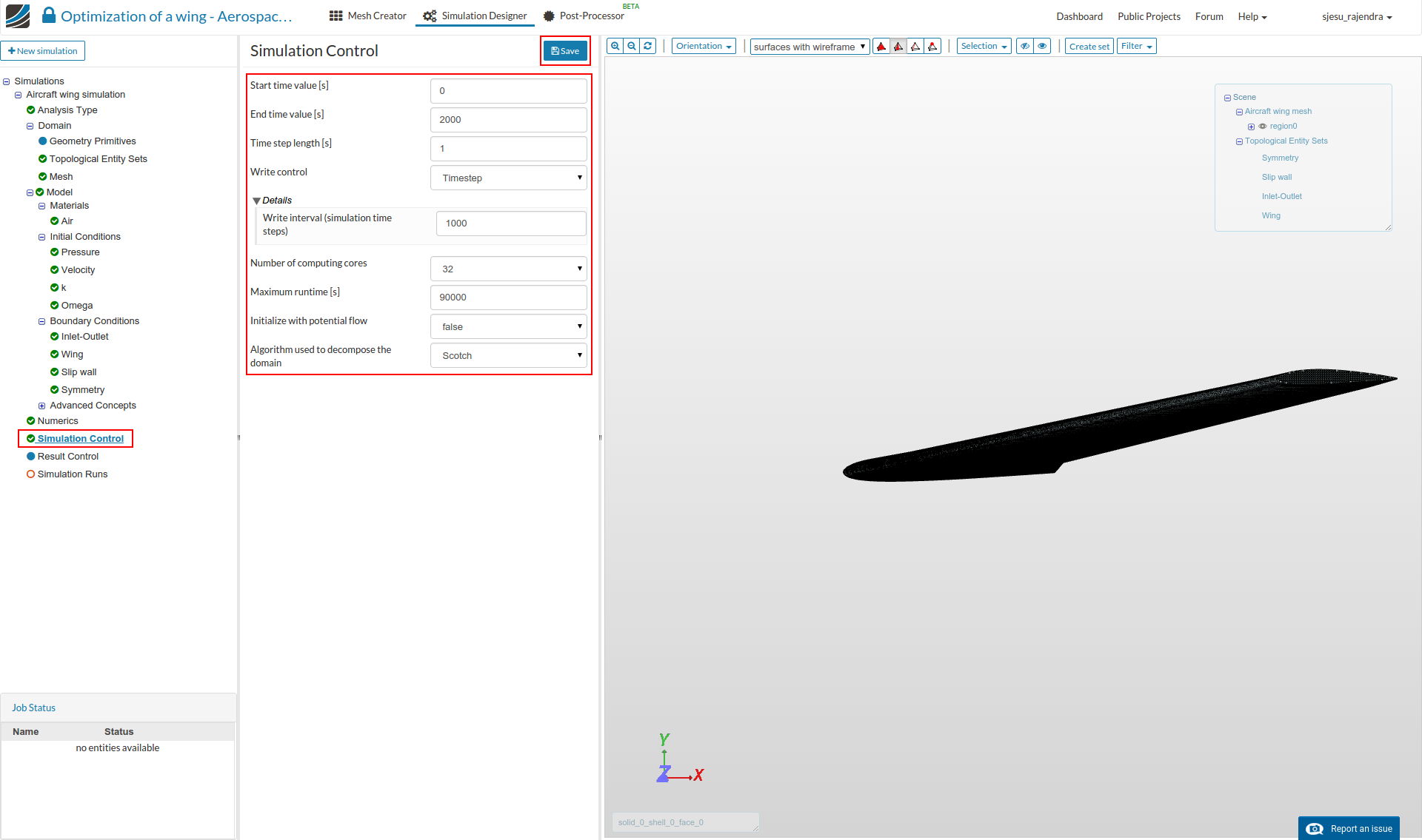
Simulation Control
- Click on ‘Simulation control’ and setup the simulation run for 2000s time with a time step of 1.
Result Control
-
Result control items help us get the surface, force and moment data out of the simulation.
-
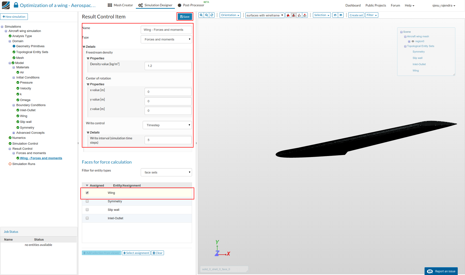
Select Result Control and select New against ‘Forces and moments’.
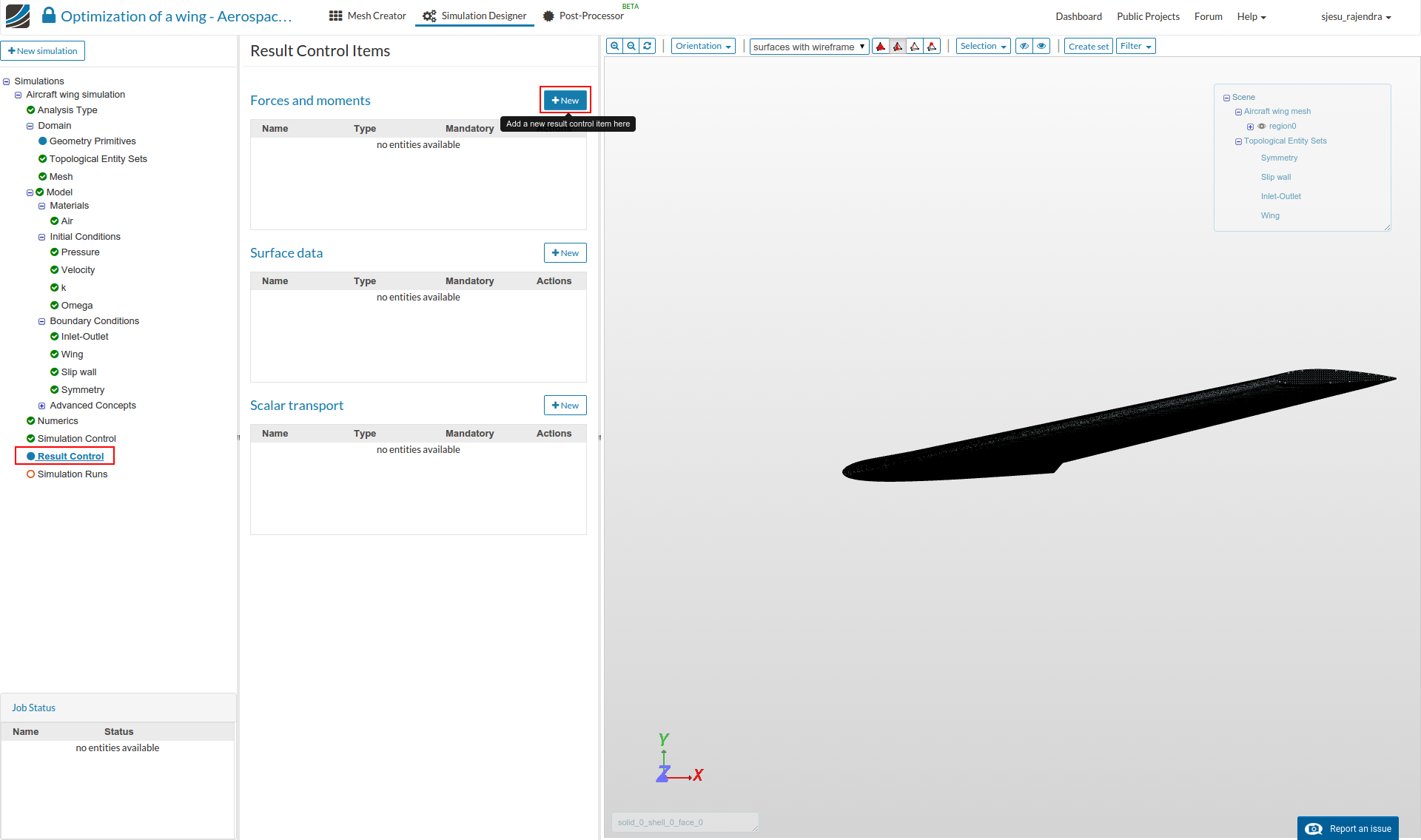
- Add the forces and moments type, with a density value of 1.2 kg/m3. Select the Wing ‘face set’ and click the Save button.
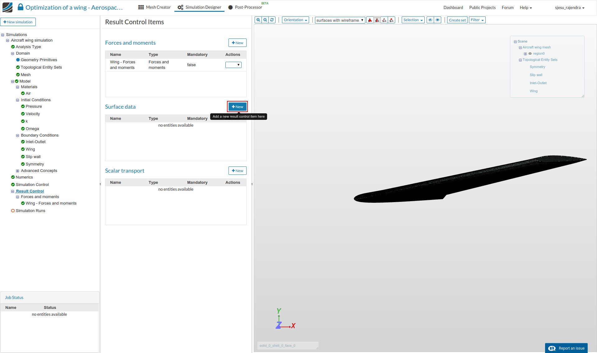
- Add another ‘Surface data’ under result control items.
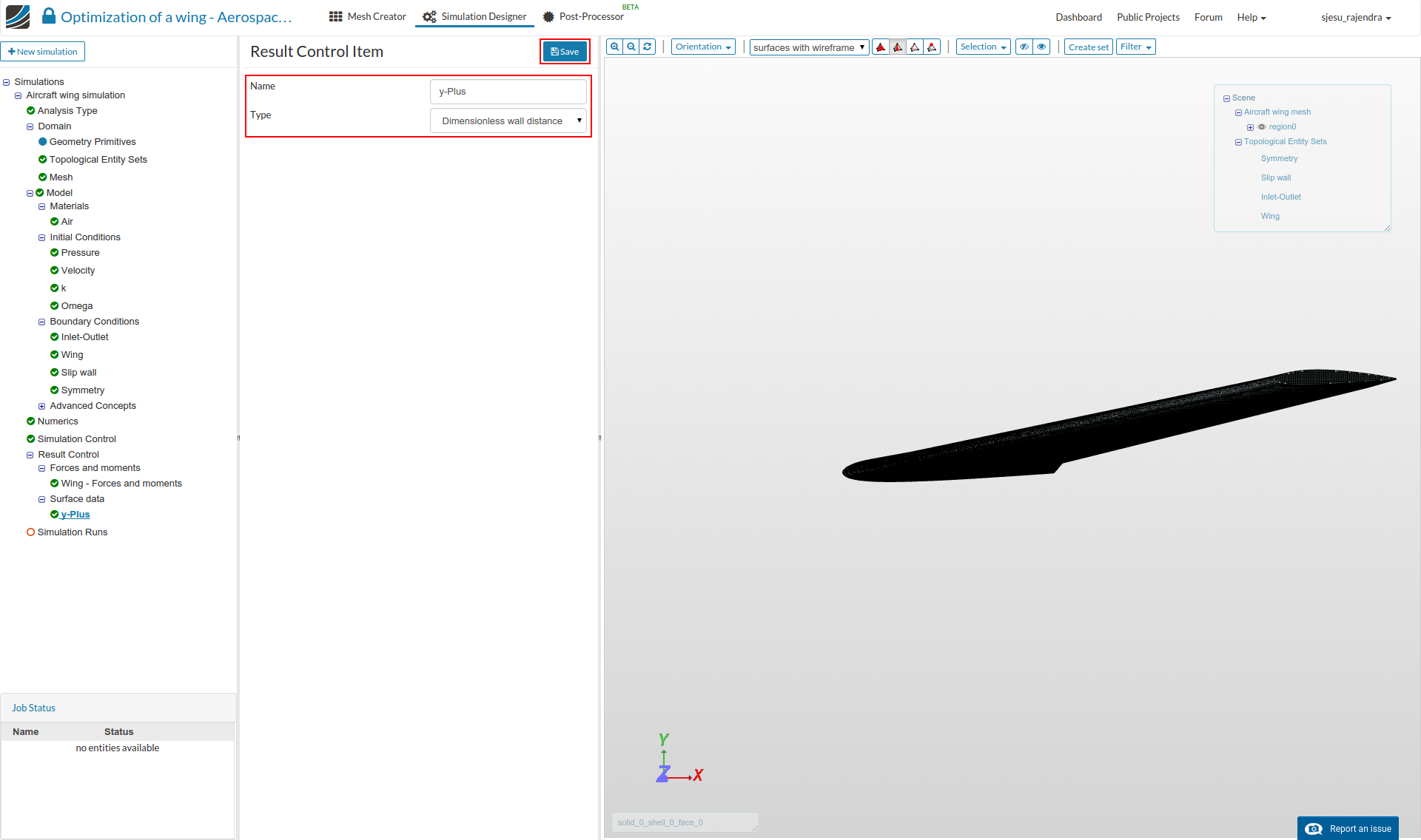
- Select the Dimensionless wall distance (y+) and click the Save button.
Create New Run
- Click on Simulation runs to create a new run and start the simulation.
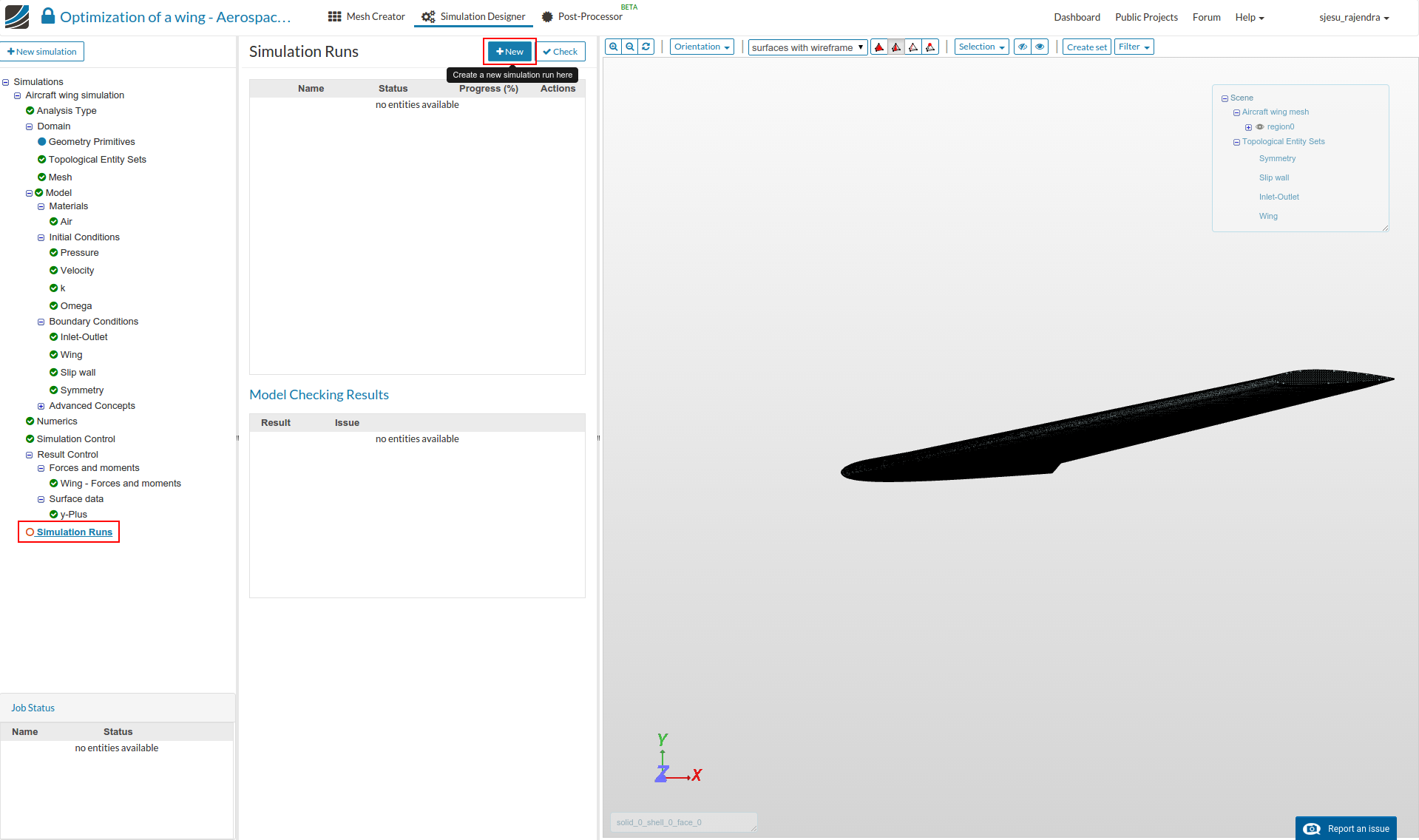
- Note that multiple simulation runs can be started in parallel. Hence you can start setting up the next case.
Aircraft blended winglet
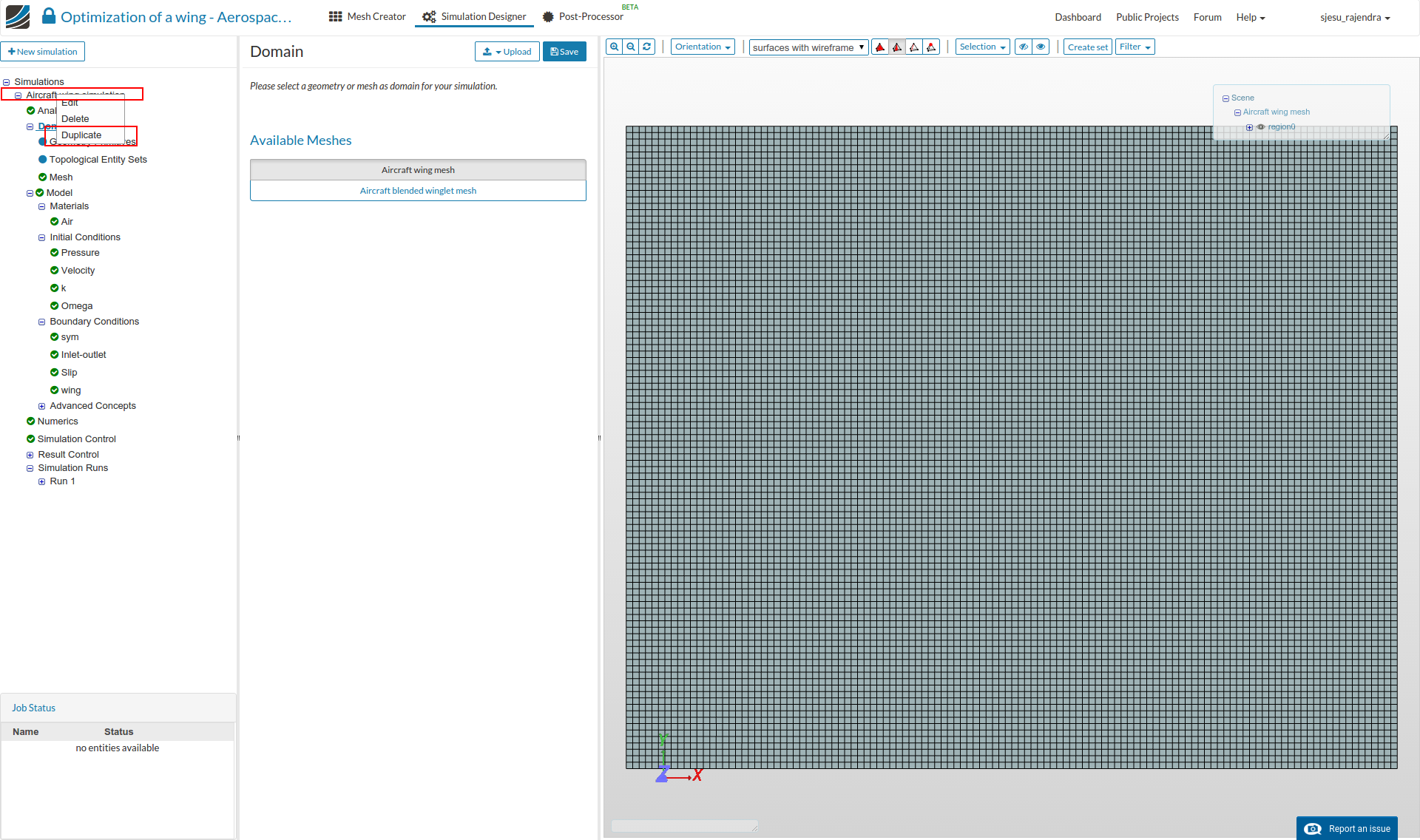
For the next set of simulations Aircraft blended winglet, duplicate the current simulation and follow these steps.
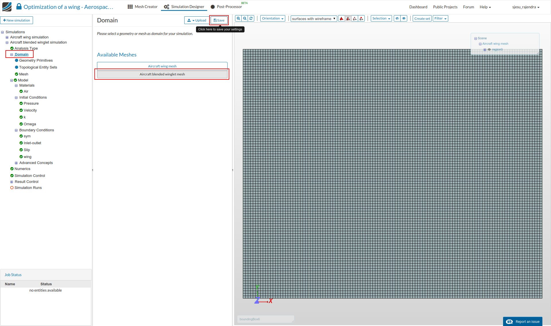
- Click Domain from the tree and select the new mesh Aircraft blended winglet mesh.
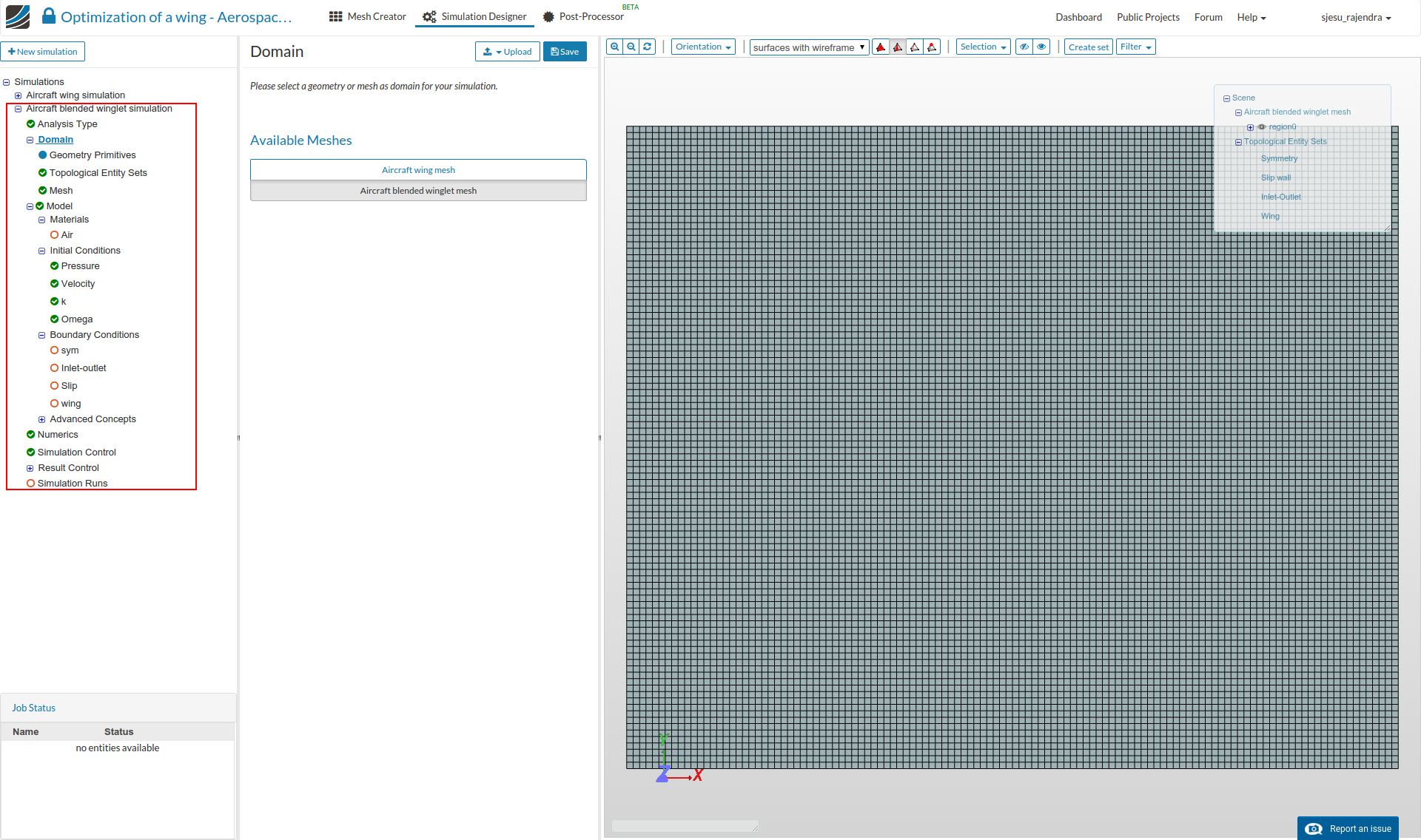
- The tree now looks as follows.
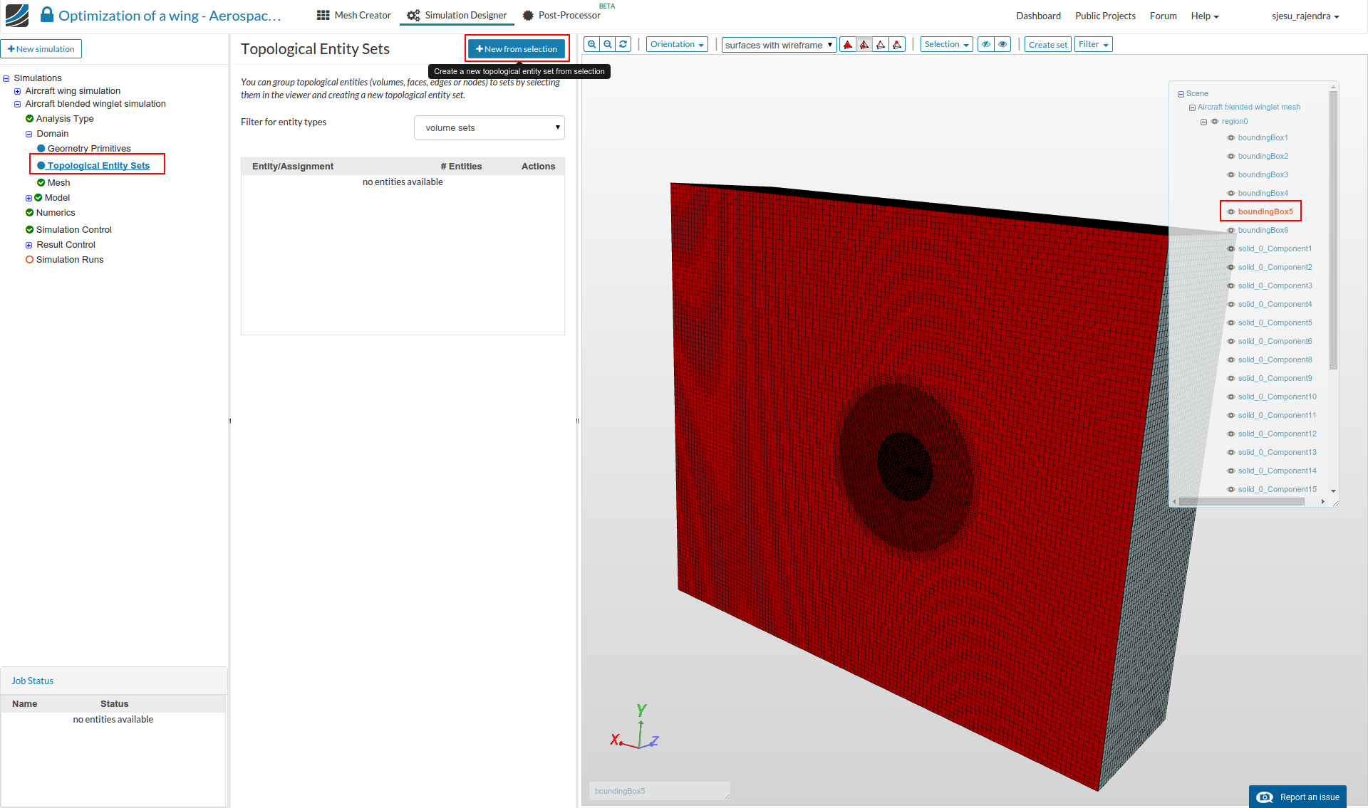
Create Topological Entity Sets
- Go to Topological entity sets and create similar sets for inlet-outlet, symmetry, slip wall and winglet for the new mesh.
Symmetry:
- Select the face as shown (boundingBox5) and click New from selection, naming it as Symmetry.
- Now select this entity which is created and click Hide selection button.
- Select the face shown (boundingBox6) and name it as Slip wall. Similarly hide this face after naming it.
- Now choose the 4 walls (boundingBox1, boundingBox2, boundingBox3 and boundingBox4), and create an entity called Inlet-Outlet. Hide this selection as well.
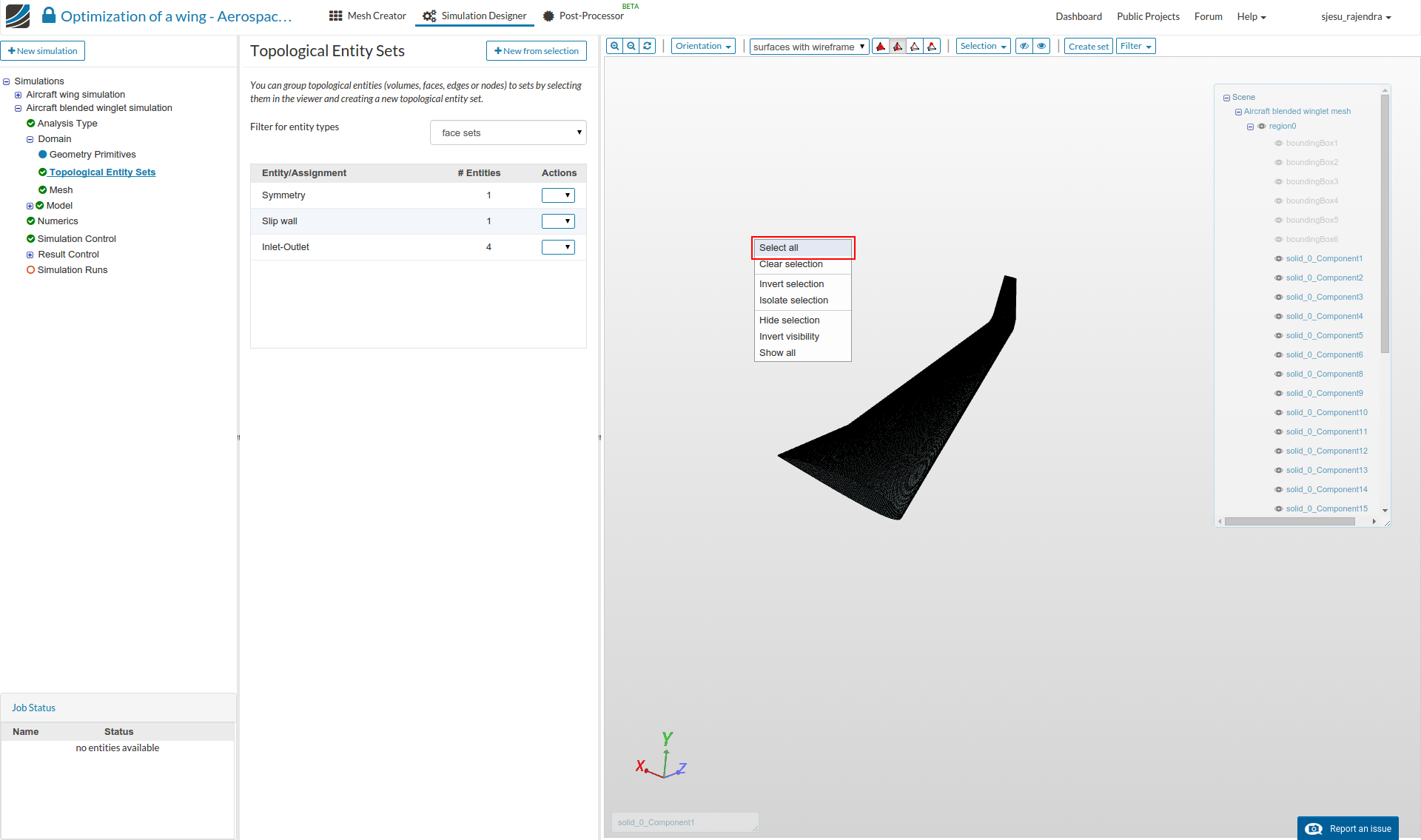
- Now right click in the viewer and click Select all, and name this entity as Winglet**.
-
Assign the material air to the new region, similar to that of the previous setup.
-
Assign the boundary conditions to the new topological entities created.
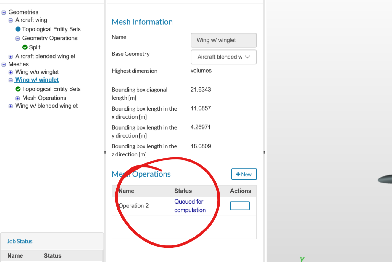
- The simulation takes between 160 to 200 mins to finish.
Post-processing
- Once the simulation is over switch to obtain the results by clicking on Post-processor tab on the top. Select the solution field (Run 1 in this case). Note that the solution field by default includes the internal mesh.
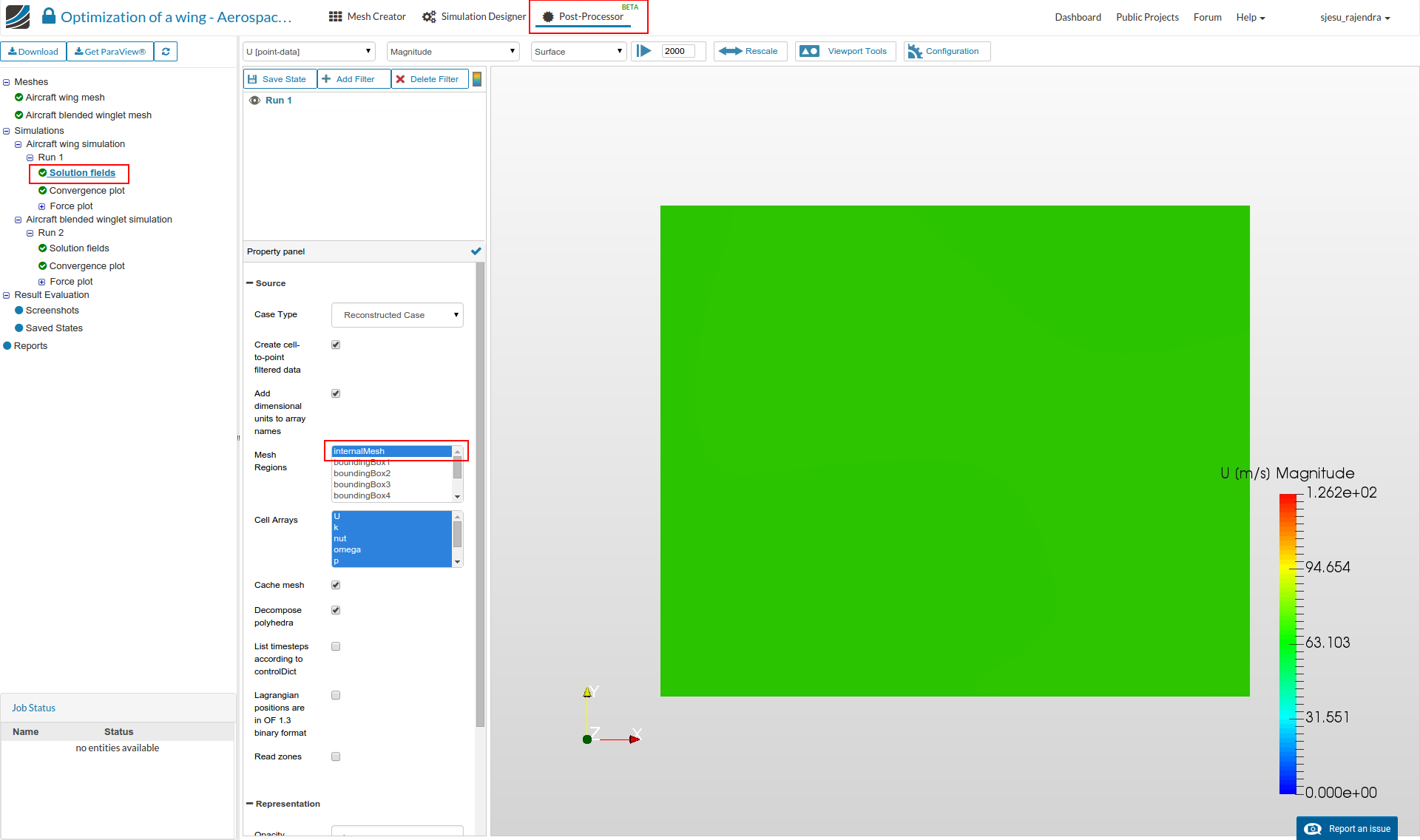
- Surface contours needs to be plotted. In order to do this, right click on the solution field and select Add result to viewer. This by default introduces another internal mesh.

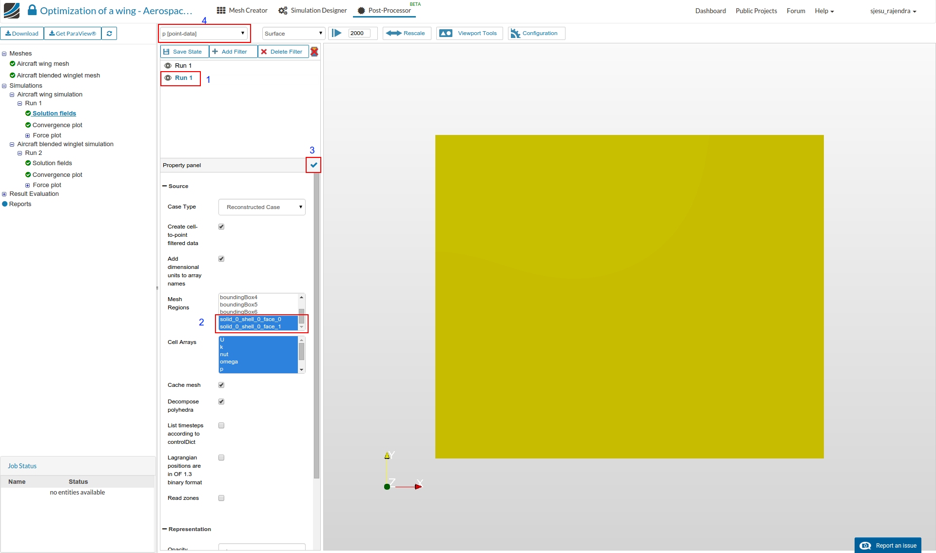
Surface contours:
-
Go to Mesh Regions from the property panel and select all the surface walls of the wings, i.e. solid_0_shell_0_face_0 and solid_0_shell_0_face_1. Select the Tick to apply.
-
Now select field as pressure p [point-data].
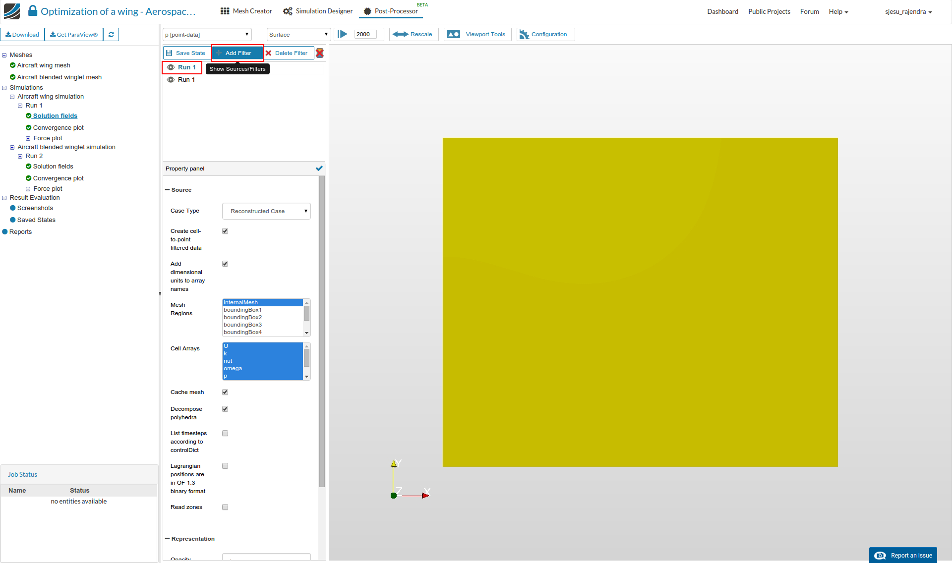
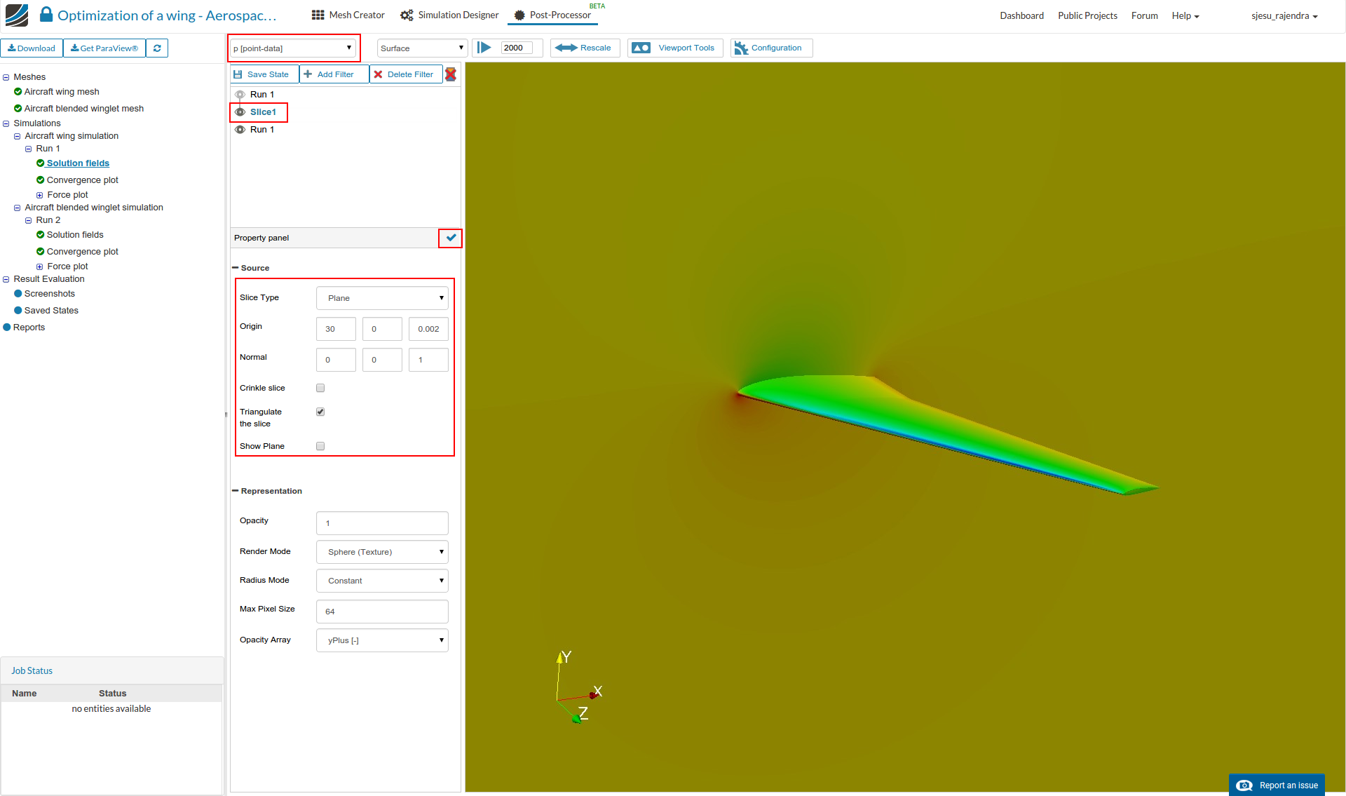
Slice Filter (2D):
- Select the internal mesh solution field ‘Run 1’ and click Add filter option to select Slice. We include a slice to the domain in order to see the pressure contour.
- Apply the following slice properties and click the ‘Tick’ icon to apply.
Slice type - Plane
Origin - default values (30, 0, 0.002)
Normal - (0, 0, 1)
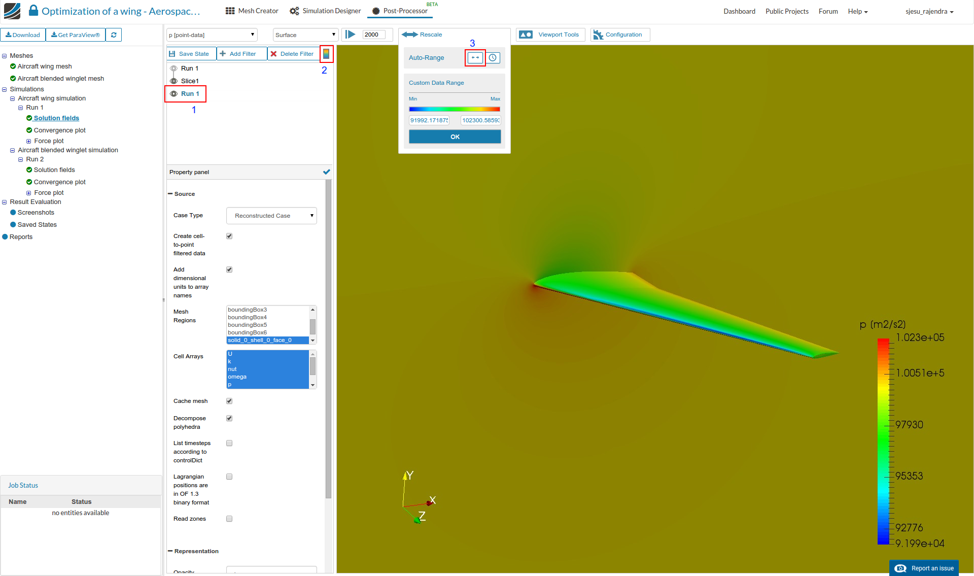
- Select the pressure data p [point data]. Click on the ‘Color bar’ below the selection panel to view the ‘legend’ bar and re-scale to auto range.
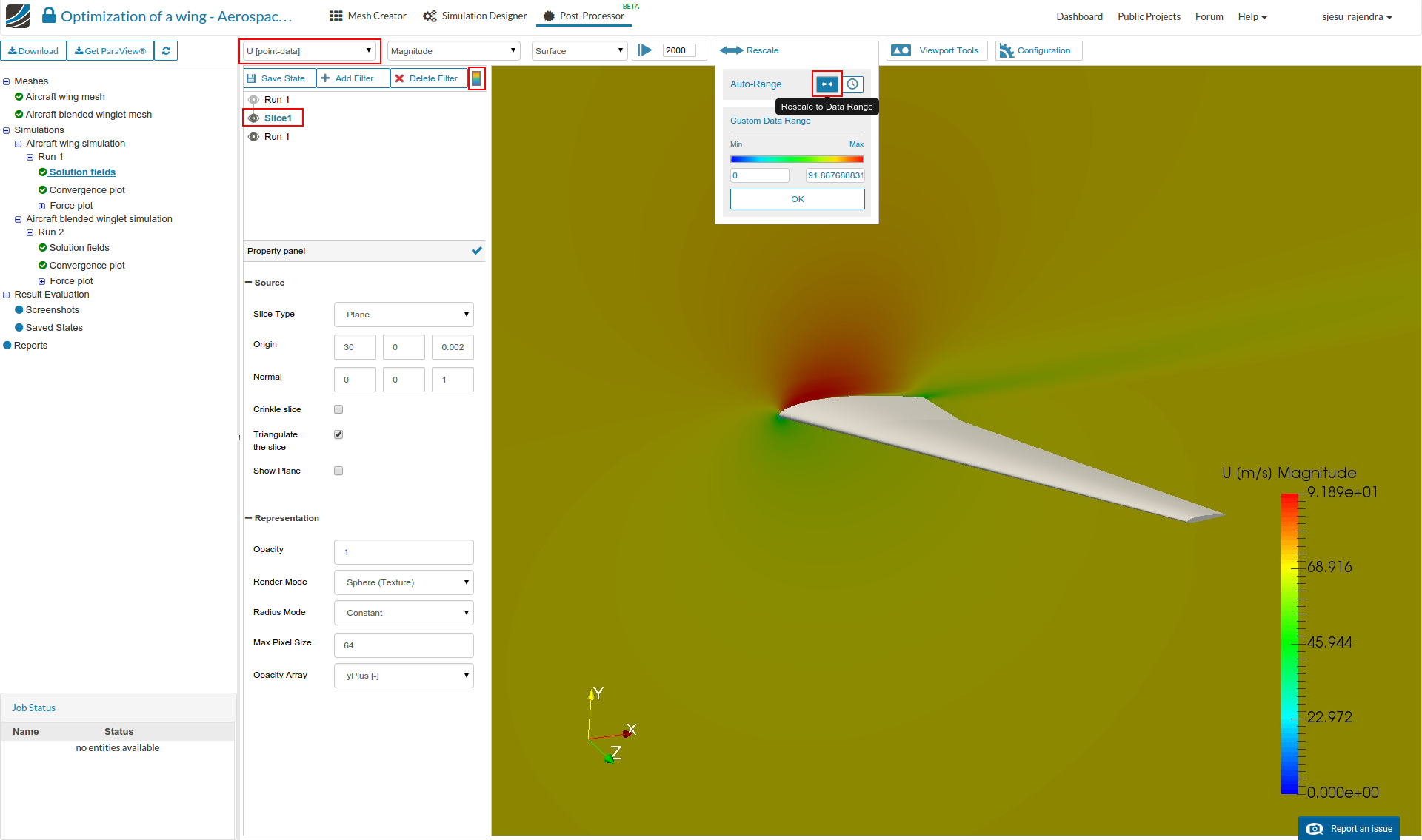
- Change the field to U [point-data] to see the velocity contour.
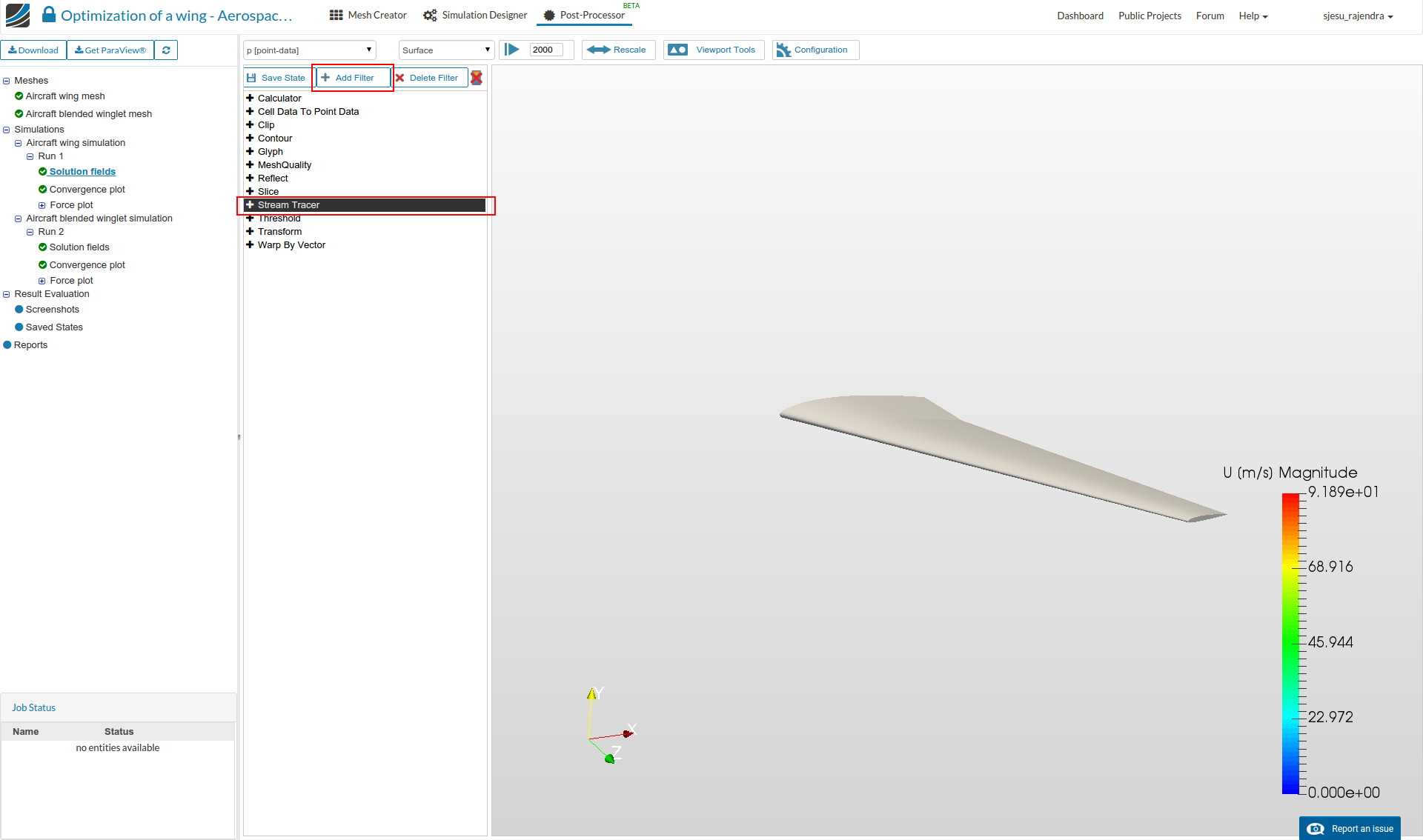
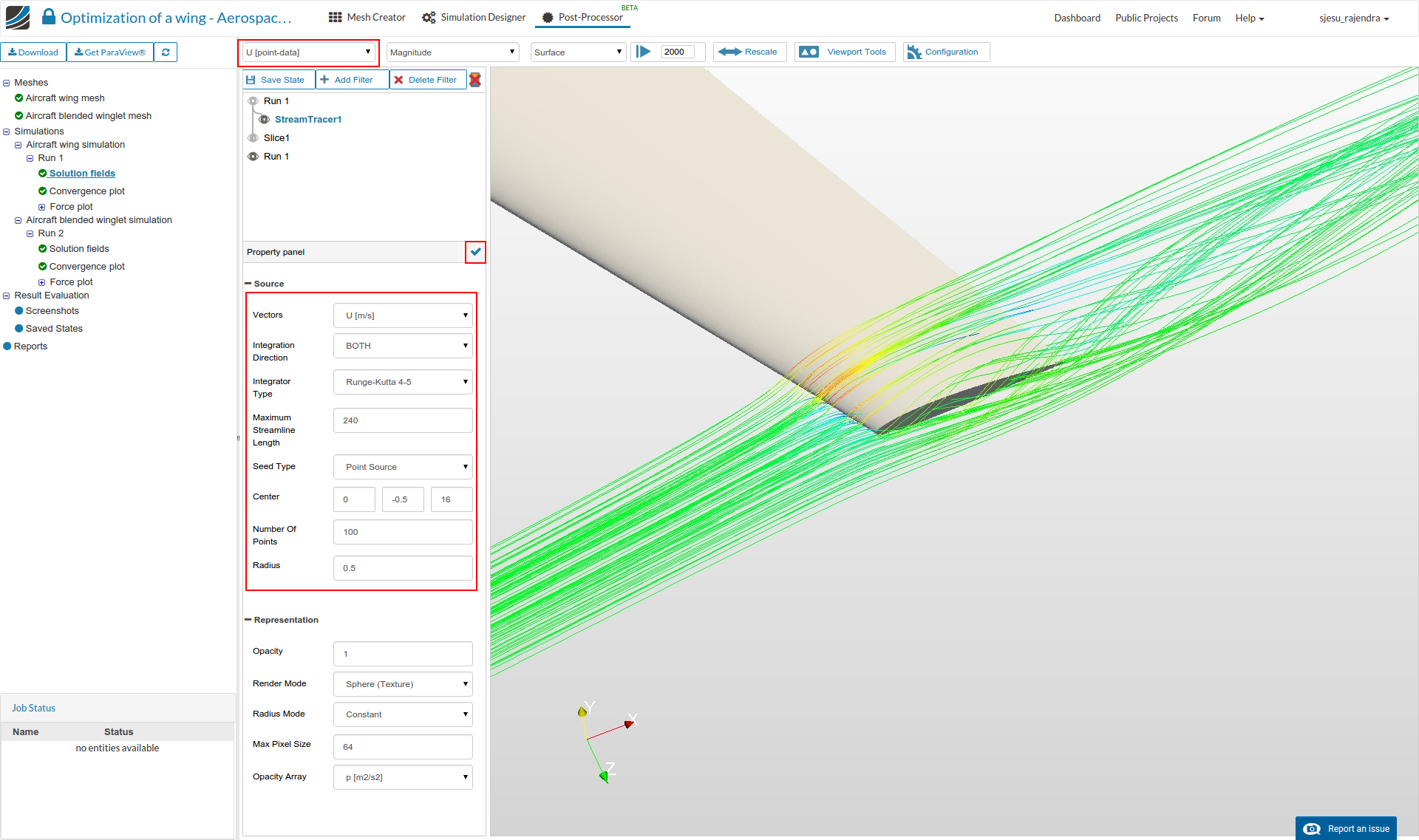
Streamlines:
- Hide the slice by clicking the small round next to the slice. Select the internal mesh solution field and click Add filter, for inserting Stream tracer in order to get the flow streamlines. Change the display field to U [point data] and enter the following values to create a point source stream tracer (Please leave the other properties with default values).
Vectors - U
Maximum Streamline Length - 240
Seed Type - Point Source
Center - (0, -0.5, 16)
Number of points - 150
Radius - 0.5
- Click the ‘Tick’ icon to apply.
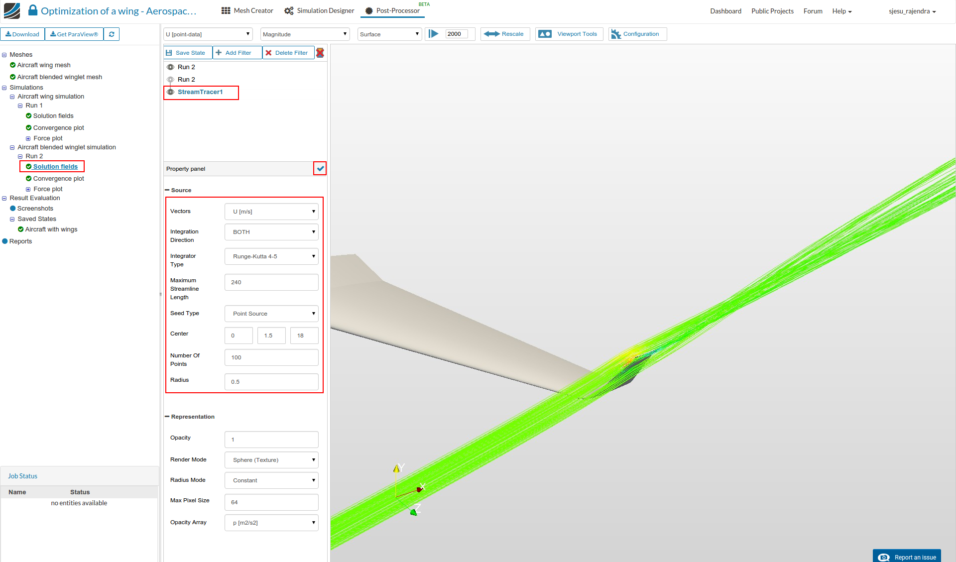
- Similarly perform the post-processing of the other configuration and compare!
 That was a typo and I’ve updated the values now. Please use the values shown in the image.
 in order to limit your simulation that it does not run forever, burning down all your core hours.
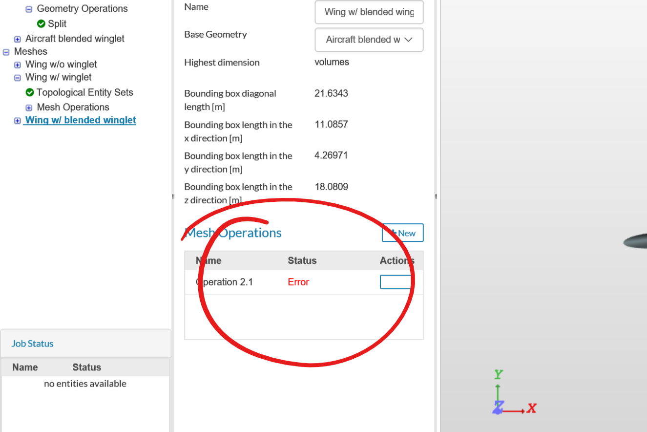
 … I don’t see the error run in your project. Is it already deleted? Could you please let me know if you tried to run the case again?