The purpose of this simulation is the examining of the behavior of air flow through a modern urban landscape. CFD wind engineering, constitutes a valuable source of input for urban developers, architectural designers and environmental planners to promote natural ventilation, a good measure for reducing energy use in buildings and providing better outdoor air quality.
You can have a look at the finished project here.
Part 1. Prepare the CAD Model and Select the Analysis Type
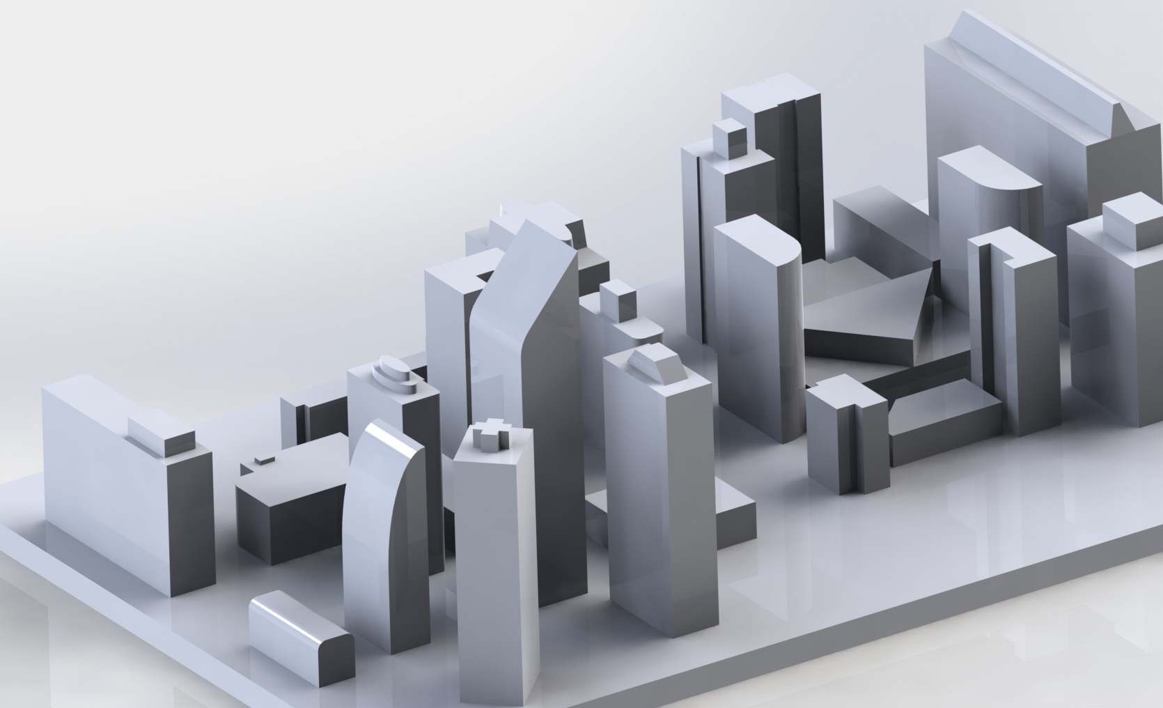
The Geometry used is a 3D configuration of buildings, forming an urban landscape.
The first step is to click on the button below. It will copy the tutorial project containing the geometry into your workbench.
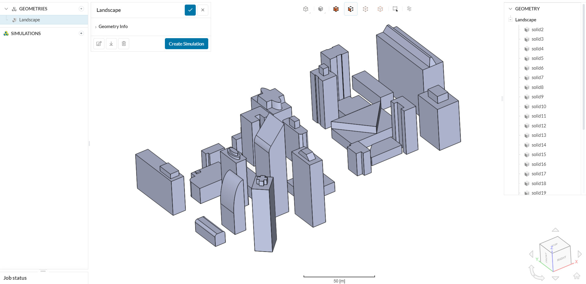
The following picture demonstrates what should be visible after importing the tutorial project:
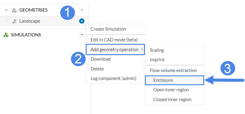
1.1. Create an Enclosure
The first step for this simulation is the creation of an enclosure. This will create the flow domain that will be used for the external aerodynamics analysis.
Select ‘Add geometry operation’ , then pick the ‘ Enclosure ‘ operation.
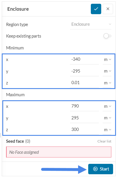
The enclosure dimensions are chosen according to the height (h) of the tallest building. As a rule of thumb, the following values can be used:
- Downstream: 8-10 times the length of the vehicle;
- Upstream: 3-5 times the length of the vehicle;
- As much as necessary to the minimum z-direction, so that the ground can be tangent to the wheels;
- Other directions: 3 times the length of the vehicle.
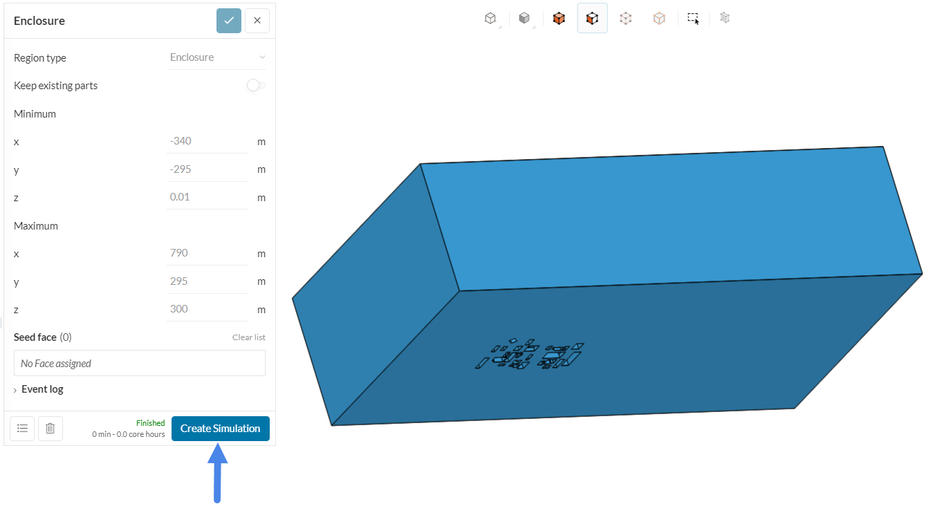
Apply the following dimensions and click ‘Apply’:
1.2 Create the Simulation
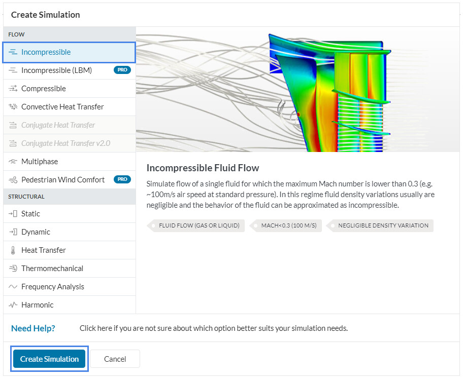
The following figure shows the resulting enclosure. Proceed by clicking on the ‘Create a Simulation’ button.
Choose the ‘Incompressible’ analysis type on the menu that appears. This is for cases where the maximum Mach number reached during the simulation is < 0.3:
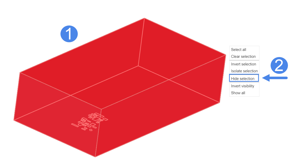
1.3 Create Topological Entity Sets
To help you later with your set up, you will create two topological entity sets. Initially, hide the six bounding faces of the domain by manually selecting them, then right-clicking on the workbench and applying the ‘Hide selection’ option:
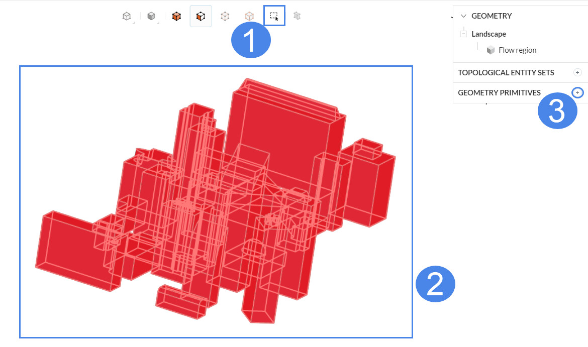
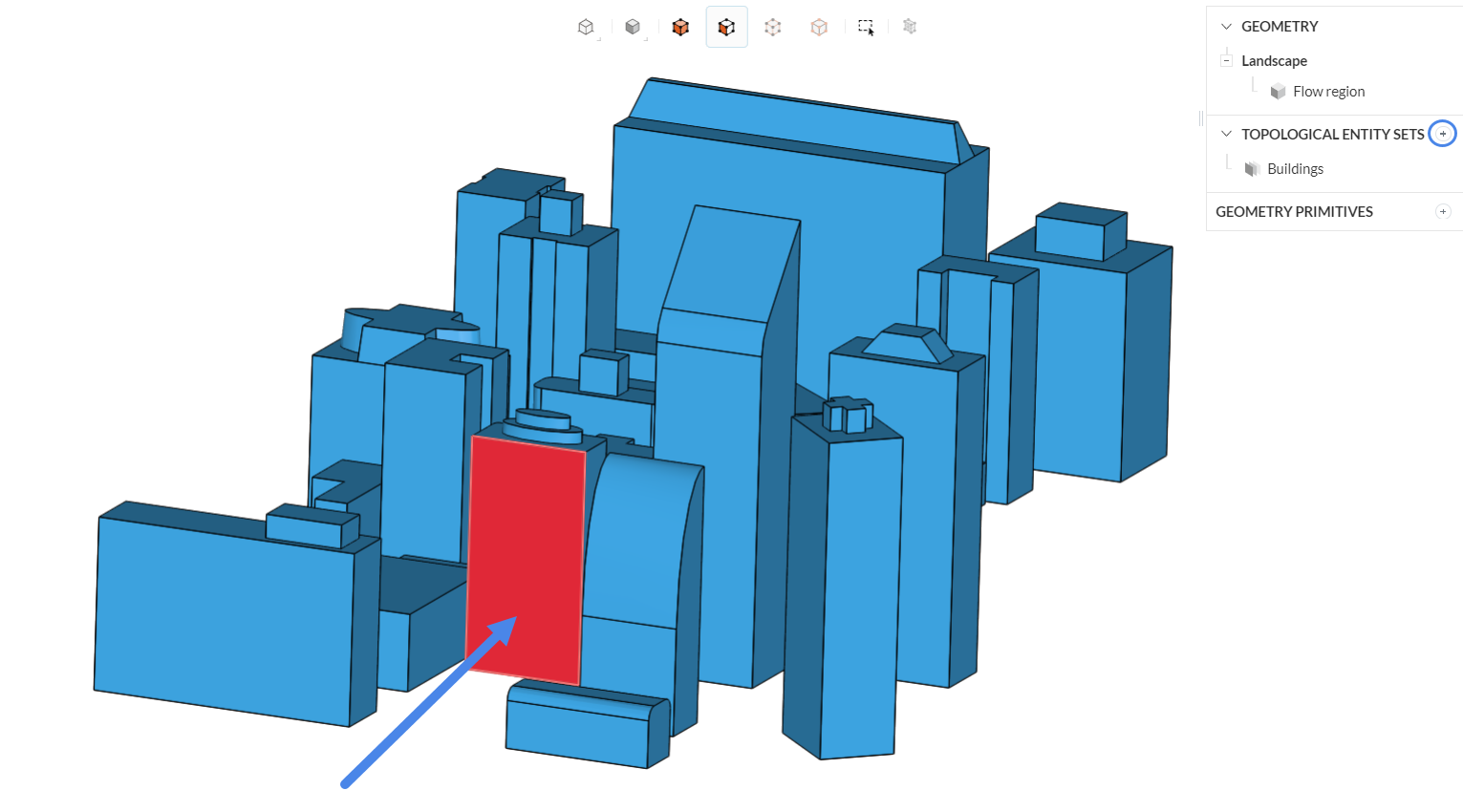
Activate the box selection, drag the cursor across the workbench until the buildings are selected (turned to red), and then click on the ‘+’ icon next to the Topological Entity Sets. Name the set as ‘Buildings’:
Create another set by clicking on the following face, and name it as ‘Facade’. This will be later used to evaluate the pressure on the surface:
Part 2. Assigning the Material and Boundary Conditions
Now we are ready to set up the physics of the simulation.
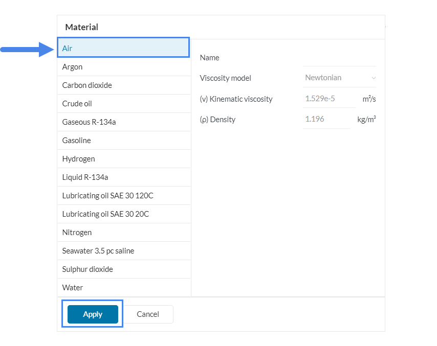
2.1 Define a Material
In the simulation tree, click on the ‘+ button’ next to Materials .

Choose ‘Air ‘ in the panel that pops up.
2.2 Assign the Boundary Conditions
In order to add a new boundary condition, click on the ‘+’ icon next to the Boundary conditions.
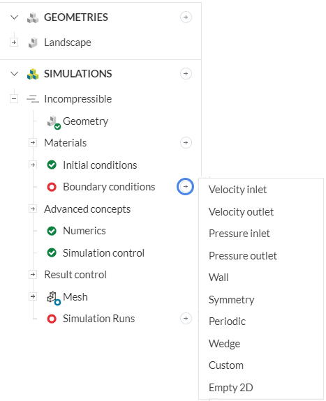
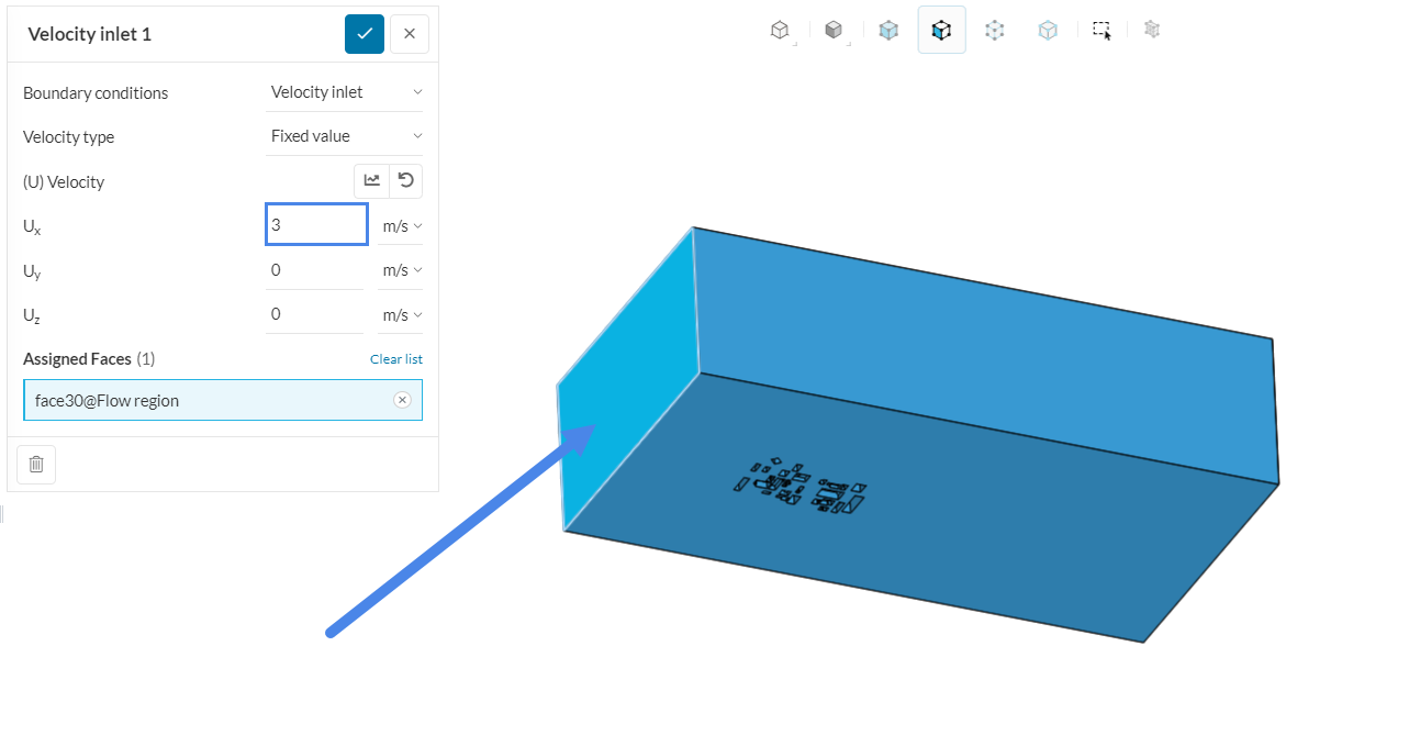
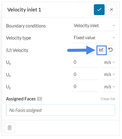
a. Velocity Inlet
Two approaches were simulated starting with a fixed uniform value of 3 m/sec:
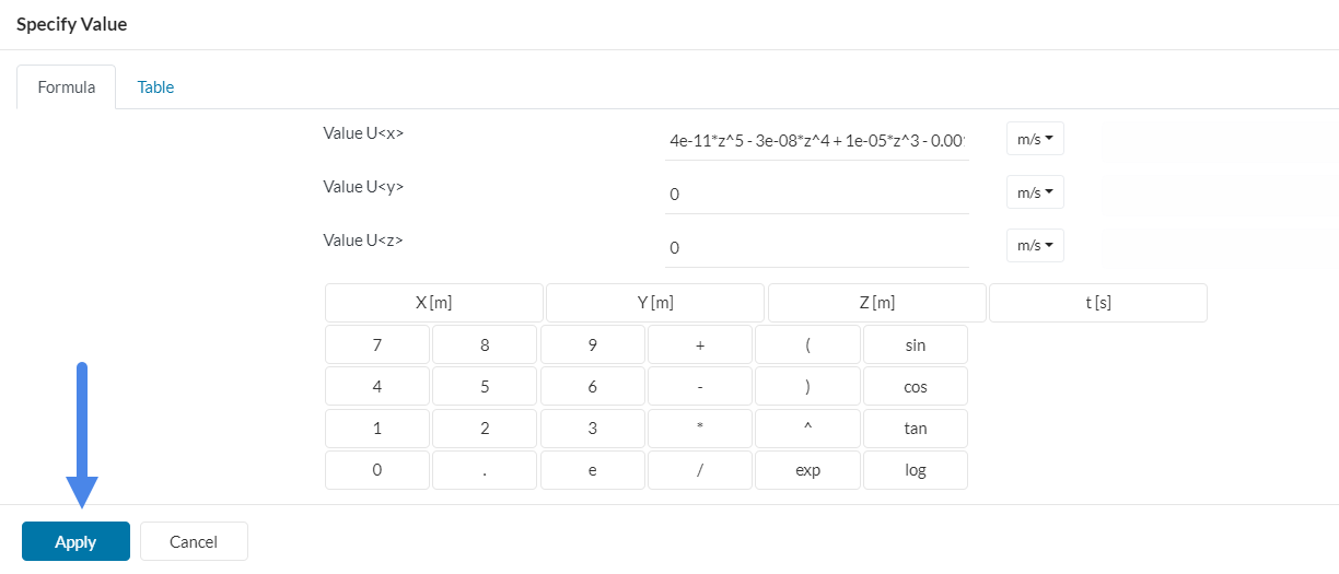
In a second simulation a velocity profile was added instead, by adjusting the data of a curve to a formula:
4e-11z^5 - 3e-08z^4 + 1e-05z^3 - 0.0014z^2 + 0.0911*z + 0.7181
by adding specified values as inlet:
And applying the formula to the x direction:
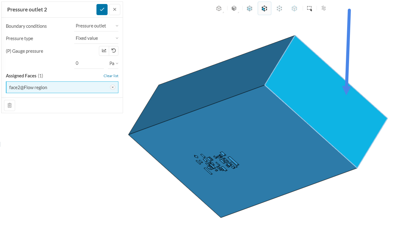
b. Pressure Outlet
Create a second boundary condition, this time a ‘Pressure Outlet’ . In incompressible analysis, the user has to specify a gauge pressure . The gauge pressure is relative to a reference value (ambient pressure, for example).
Therefore, a pressure outlet condition with 0 ¶ gauge pressure is applied to the outlet face of the domain:
c. Slip Walls
Make sure that the top, right and left side of the domain are set as slip walls, so they are modeled like open air environment:
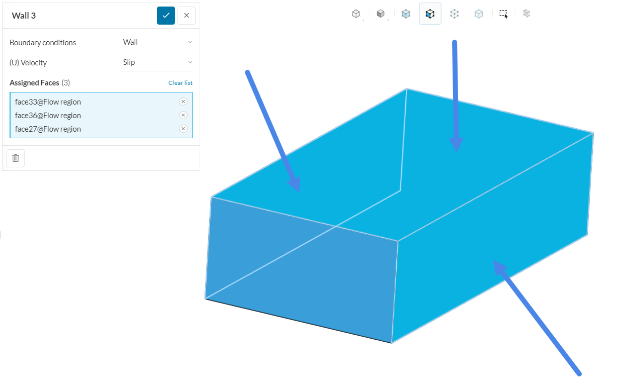
Keep in mind that the faces that did not receive a boundary condition, will be automatically assigned as no-slip walls.
2.3. Set the Numerics & Simulation Control
The Numerics settings can be left as default. If you use your own model and have a large mesh, make sure to set the ‘Maximum runtime’ input ion the Simulation Control tab to 30000 sec, so that there is no way the simulation is interrupted.
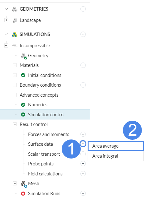
2.4 Results Control
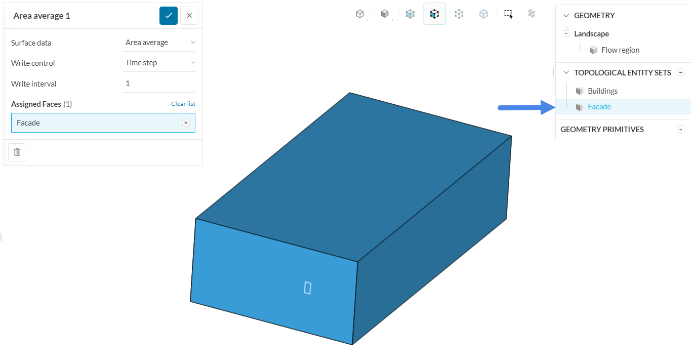
Create a ‘Surface data’ set for the Facade, so you measure the average pressure on the face.
Assign it to the face of interest by clicking on the ‘Facade’ on the Geometry tree at the right of the page:
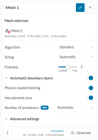
3. Mesh
For the meshing operation, you will use the recommended the standard algorithm. The standard mesher is a good choice in general, as it is quite automated and delivers good results for most geometries, with the default properties.
3.1. Add Refinements
Proceed to create new geometry primitives for your refinements. Click on the ‘+ button’ next to the Geometry primitives in the right-hand side panel:
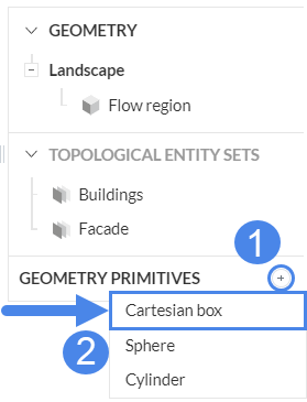
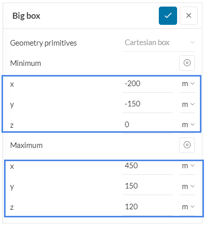
First you will ad teh dimensions of the large cartesian box:
Then create a smaller cartesian box:

To create a new refinement, click on the ‘+’ icon next to the Refinements, and select the type you wish to add:

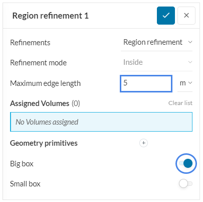
a. Region Refinements
A region refinement is used to refine the volume mesh for one or more user-specified geometry primitives . You will create one for each cartesian box. For the large box apply a maximum edge length of 5 m:
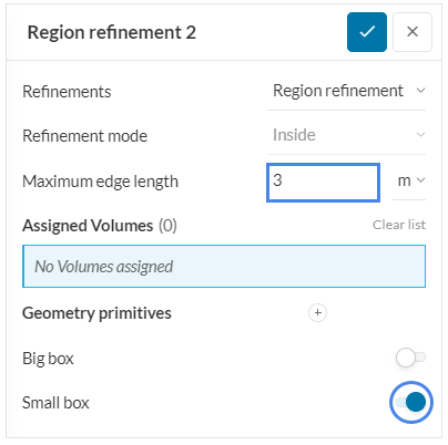
Repeat for the small box, and this time apply a maximum edge length of 3 m.:
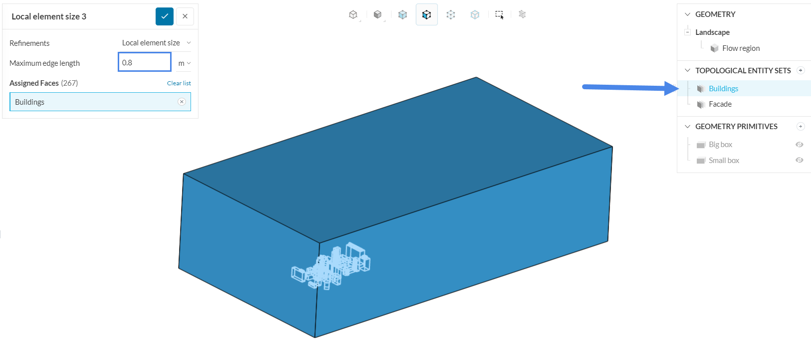
b. Local Element Size
This refinement adds a restriction to the maximum edge of the cells, limiting their size. Use a maximum edge length of 0.8 m , and apply it on the buildings, by selecting them in the geometry tree:
You can then go back to the Mesh tab and click on the Generate option, so the creation process begins. After 23 minutes, a mesh consisted of 6.8 m cells will be ready to use.
4. Start the Simulation
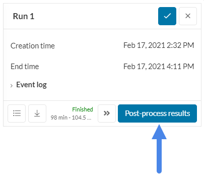
Proceed to start the run, by clicking on the ‘+ button’ next to Simulation Runs :
After 80-100 minutes (depending on the velocity inlet method you used), the run will be finished, and you can post-process your results.
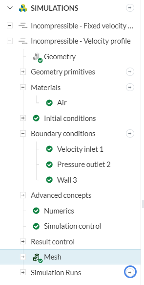
5. Post-Processing
Following the ending of the simulation, you can start to extract and analyze the results, by expanding the section of 'Run 1’. Here the results of the simulation with the fixed velocity value for the inlet are investigated:
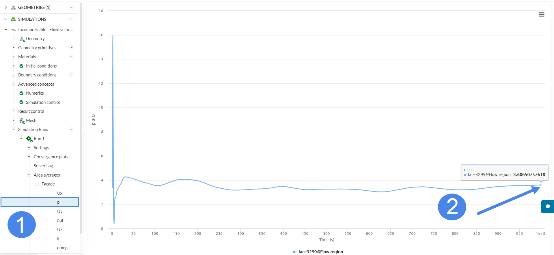
5.1. Average Pressure Data
After the simulation is finished, you can check the Pressure distribution on the façade. Use the final value, as this is the converged solution:
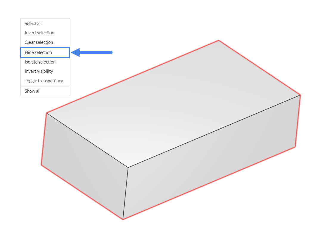
5.2. Surface Visualization
Enter the post-processor in order to visualize the values of the parameters on the domain:
To hide the walls of the domain, click on each one of them, then right-click on the workbench and choose the ‘Hide selection’ option, to turn them invisible:
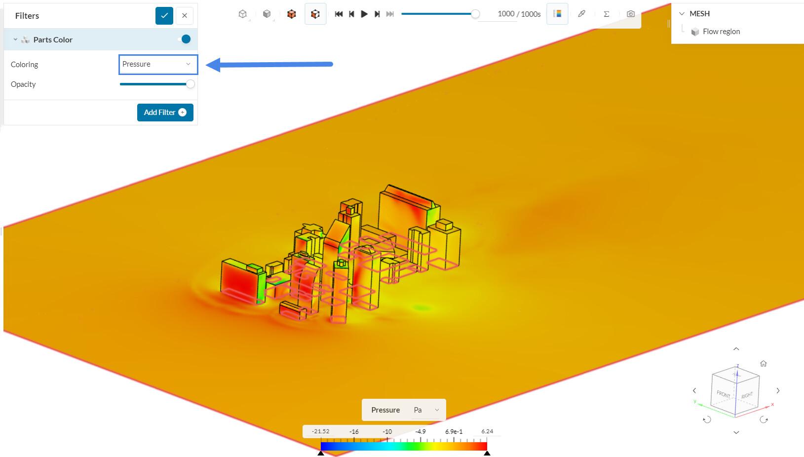
Set the Coloring to ‘pressure’. You can check all the other field parameters as well too:
5.3 Cutting Planes
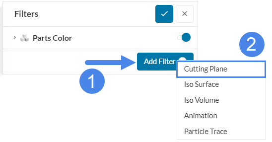
In order to observe the flow behavior inside the domain, add a new filter, and select the ‘Cutting plane’:
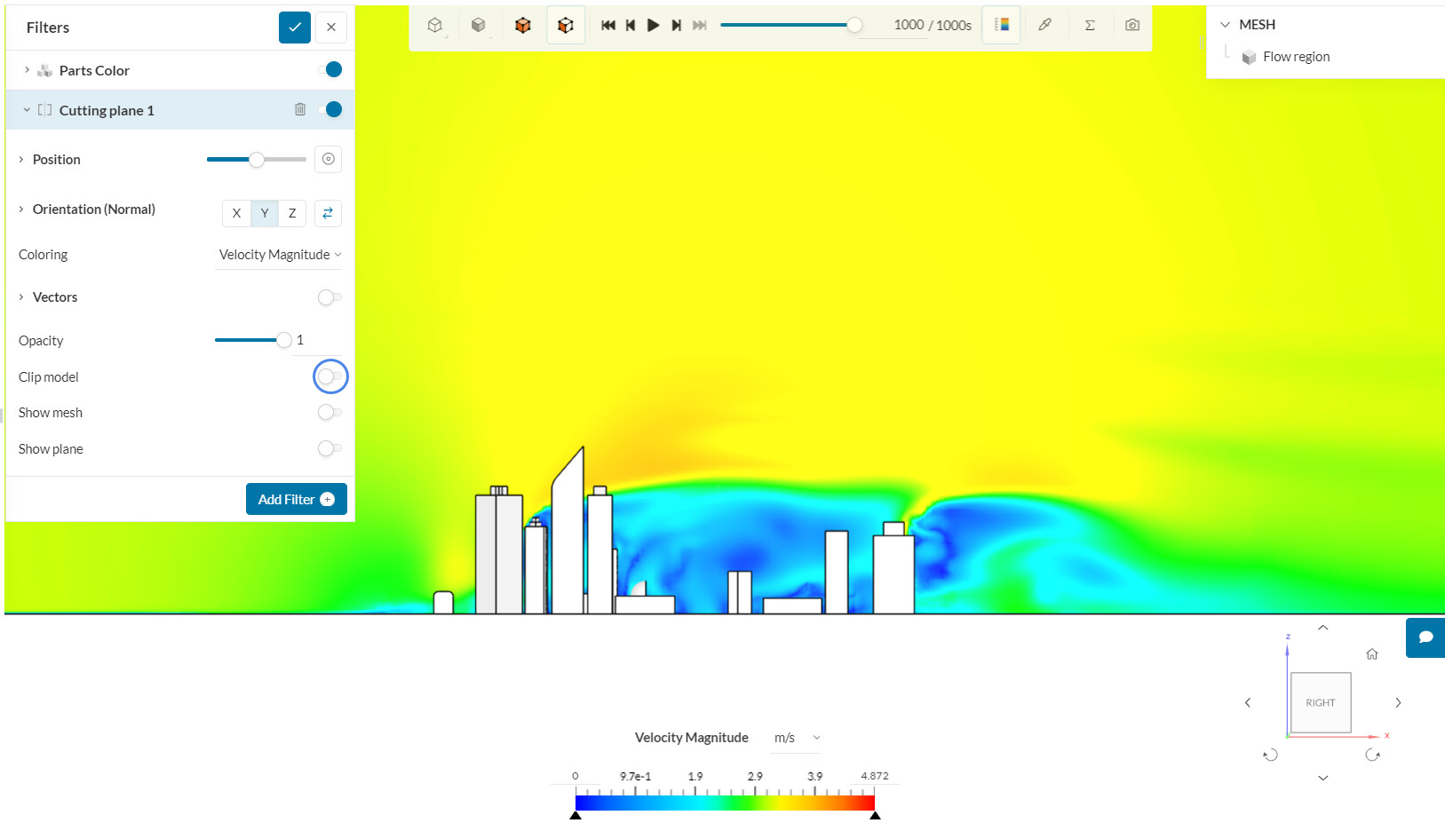
Leave the settings at default, and de-activate the ‘Clip mesh’ option, so all the 3D buildings are visualized:
You can analyze the aerodynamic flow results further with the SimScale post-processor. Have a look at our post-processing guide to learn how to use it.
Congratulations! You finished the wind field over city landscape tutorial!