
In fluid dynamics, a turbulent regime refers to irregular flows in which eddies, swirls, and flow instabilities occur. It is in contrast to the laminar regime, which occurs when a fluid flows in parallel layers, with no disruption between the layers.
The turbulence regime is extremely frequent in natural phenomena and human applications; some examples are the rise of cigarettes’ smoke, waterfalls, and most of the terrestrial atmospheric recirculation. In terms of human applications, turbulent regime occurs in the aerodynamics of vehicles, but also in many industrial applications such as heat exchangers, quenching process or continuous casting of steel.
Reynolds Number
The real onset of scientific studies on turbulence can be found in the work of Osborne Reynolds in the second half of the 19th century. Reynolds showed the transition between a laminar and a turbulent regime through a set of experimental investigations. He also suggested that this transition was directly linked to the ratio between inertial and viscous forces. This ratio was computed by George Gabriel Stokes in 1851 and has been named “Reynolds number” in honor of Osborne Reynolds who popularized it. This dimensionless number is defined as:
where:
- \rho is the density of the fluid
- u is the macroscopic velocity of the flow
- d is the characteristic length of the involved phenomenon
- \mu is the dynamic viscosity of the fluid
- \nu is the cinematic viscosity of the fluid.
Turbulent flows occur when Re exceeds a certain threshold (dependent on the application’s topology and physics) called “critical Reynolds number”.
Turbulence structure
In 1920, Lewis Fry Richardson summarized his works about the structure of turbulence for meteorological applications through a celebrated rhyme published in Weather Prediction by Numerical Process$^1$:
“Big whirls have little whirls that feed on their velocity,
and little whirls have lesser whirls and so on to viscosity”.
This principle was motivated by energetical considerations; big eddies are highly inertial and tend to be unstable. Their motion feeds smaller eddies thanks to a local transfer of kinetic energy. These smaller eddies undergo the same process, giving rise to even smaller eddies which inherit the energy of their predecessor eddy, and so on. This transfer of energy is usually called “energy cascade” and it is mainly inertial, thus almost no energy dissipation occurs until reaching a sufficiently small length scale such that the viscosity of the fluid can effectively dissipate the kinetic energy. This latter scale of the turbulence exhibits a local laminar regime and is characterized by a low value of Re. This process has been depicted in figure 2; Richardson studies highlight an important feature of turbulent flows: they are energy demanding. A turbulent flow will dissipate energy and decay to a laminar flow unless it is fed by an external source of energy.
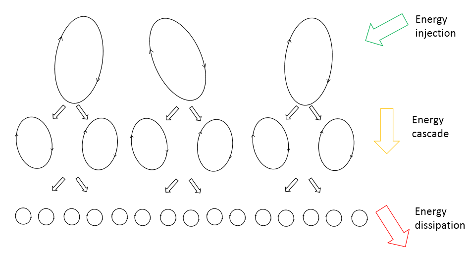
Figure 2: Richardson’s energy cascade
Governing Equations
Turbulence scale
The complexity of turbulence and its aleatory behavior led scientist to use statistical models to describe turbulence flows. In 1941, Kolmogorov enhanced Richardson theory[2]. Kolmogorov postulated that for high enough Reynolds number, the small scale eddies are isotropic, while large eddies may be anisotropic (or anyway, dependent on the specific domain’s topology). This assumption is very important because it means that the statistical analysis of small eddies is independent of any specific geometry, thus it is universal for all turbulent flows. Under this hypothesis, Kolmogorov statistically described the main features of the smallest turbulence scale (known as “kolmogorov microscales”) as follows:
- Kolmogorov length scale: \eta = \left(\frac{\nu^3}{\epsilon}\right)^{0.25}
- Kolmogorov velocity: \tau=\left(\frac{\nu}{\epsilon}\right)^{0.25}
- Kolmogorov velocity scale: u=\left(\nu\epsilon\right)^{0.25}
RANS
It is normally believed (but not proved) that Navier-Stokes equations model any kind of flow, turbulent flows included. The problem is that for very high values of Re, the resolution of NS equation is very challenging and not stable, thus a small perturbation in the parameter, initial condition, or boundary conditions may lead to a completely different solution. This problem is partially overcome by the use of the Reynolds-Averaged Navier-Stokes Equations (RANS)[3].
Let’s consider the Navier-Stokes equation for an incompressible newtonian fluid:
where u is the velocity, p is the pressure of the fluid and the material parameters are considered uniform.
The principle is to consider the flow as the sum of a mean flow and a turbulent/unsteady flow; the steady mean velocity can be computed as the Favre average of the global velocity:
thus, the velocity can be decomposed as:
where U is the mean velocity and u' is the turbulent flow velocity. T is the averaging time-scale, which must be small enough to have a good approximation of the problem, but also sufficiently higher than the turbulence time-scale, i.e. the Kolmogorov’s turnover time. By substituting the averaged quantities in the Navier-Stokes equation, we obtain the RANS equations:
where \left( u_{i}' u_{j}'\right) _j is usually called “Reynolds stress” and represents the effect of the small-scale turbulence on the average flow.
The RANS equations have no unique solution because are not in a close form, the unknowns are more than the equations. Thus, additional equations are needed to close the problem. The most common strategy used in CFD is to relate the Reynolds stress to the shear rate by the Boussinesq relationship:
where \mu_t is the turbulent viscosity, which is usually computed through turbulence models$^4$.
Applications
Turbulent flows are present in many natural phenomena (e.g. river flows, atmospheric streams, natural convection) and human applications (e.g. wind flow in a city, aerodynamic analyses, continuous casting, quenching process, cooling/heating systems). In this section, two small applications done by using SimScale have been reported.
The first (figure 3) consists of the analysis of the flow around a cylinder. The case can be applied to the flow of a river around a bridge column, but it also has a great academic value since it is a widely used benchmark for validation. Furthermore, it is often used to show the different regimes (linked to the presence, size, and frequency of eddies) at different problem’s configurations.
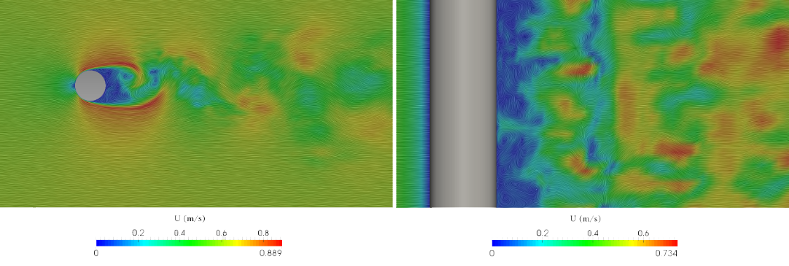
Figure 3: Contour plot of velocity in the plane normal (left) and parallel (right) to the cylinder’s axis.
The second case is the aerodynamic analysis of a vehicle (figure 4). The high velocities and the low viscosity of air encourage the development of a turbulent regime, even if it is usually avoided as much as possible in order to reduce the drag linked to the detachment of eddies behind the vehicle.
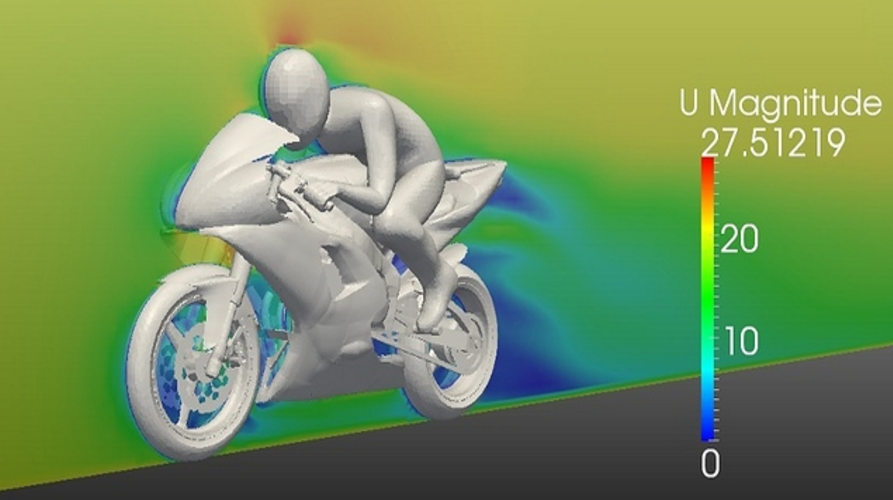
Figure 4: Contour plot of air velocity around a motorbike.
Related topics
Resources
^1: Richardson, L. F. Weather Prediction by Numerical Process (Cambridge Univ. Press, 1922)
^2: Kolmogorov originl paper on turbulence | Micropore
^3: https://web.stanford.edu/class/me469b/handouts/turbulence.pdf
^4: Turbulence modeling -- CFD-Wiki, the free CFD reference