
The transport equation describes how a scalar quantity is transported in a space. Usually, it is applied to the transport of a scalar field (e.g. chemical concentration, material properties or temperature) inside an incompressible flow. From the mathematical point of view, the transport equation is also called the convection-diffusion equation, which is a first order PDE (partial differential equation). The convection-diffusion equation is the basis for the most common transportation models.
Mathematical derivation
The transport equation (or convection-diffusion equation) can be seen as the generalization of the continuity equation ^1. While the continuity equation (extensively described in the article about incompressible flow^2) usually describes the conservation of mass, the convection-diffusion equation describes the continuity/conservation of any scalar field in any space.
Let’s consider an infinitesimal portion of space and its boundaries, as described in figure 1.
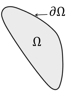
Figure 1: Generic space domain
The continuity principle states that the rate of change for a scalar quantity in any differential control volume is given by flow and diffusion into and out of that part of the system, along with any generation or consumption inside the control volume. In practice, it means that the variation of concentration of a certain quantity in the volume is given by the balance of this quantity flow across the boundary and the amount of quantity produced or removed in the volume. From the mathematical point of view, this balance is expressed by the following equation:
where c is the scalar field to be analyzed, j is the flux of c through the boundary, and S is the source/sink term inside \Omega. Equation 1 is nothing more than a balance of a scalar quantity inside the volume: the first term (\frac{\partial c}{\partial t}) represents the variation of quantity of the scalar field inside the control volume, the second term (\nabla\cdot j) represents the net balance of the quantity of field which enters and exits the control volume, and the third term (S) represents the amount of the scalar quantity “created” or “destroyed” inside the volume.
Equation 1 can be further detailed by developing its terms:
- The flux j can be divided into two terms: the convective and the diffusive terms. The convection term is the quantity of the transported field which moves across the boundaries because of the flow; thus it is proportional to the velocity and can be written as j_{convection}=cu, where c is the transported scalar quantity and u is the velocity of the means which transports this quantity. The diffusion term is the transportation of the scalar quantity according to its gradient, so j_{diffusion}=D\nabla c, where D is the diffusivity.
- The source term can be divided into a pure source term and a reaction term. The pure source term (S_S) represents the creation/destruction rate of the field inside the volume. The reaction term (S_R) describes the creation/destruction of the transported quantity as a reaction to this quantity itself; it is, therefore, proportional to the transported field and can be written as S_R=f(c), where f(c) is a function of the transported scalar field. S_R is quite uncommon for engineering applications, so it is often neglected.
Equation 1 can thus be re-written in its fully developed form as:
Heat Transfer
During thermal simulations, the temperature field (which is scalar) is transported according to the convection diffusion equation. In this specific case, the following notation is commonly used by the science community:
where:
- \rho is the material density
- c_p is the heat capacity
- T is the temperature
- k is the thermal conductivity
- Q is the volumetric heat flux
- \epsilon is the emissivity
- \sigma is the Stefan-Boltzmann constant
- A is the boundary surface in which heat is exchanged by radiation.
Equations 2 and 3 differ only for the notation and for the complexity of the reaction term, coming from the physical modelling of heat transfer phenomena$^3$.
Equation 3 is often simplified in common engineering applications thanks to the following hypotheses:
- Homogeneous material (i.e. constant and uniform material parameters):
- Incompressible flow (i.e. \nabla\cdot u=0):
- Neglection of heat exchange by radiation:
- Steady state (i.e. \frac{\partial T}{\partial t}=0):
Chemical concentration
Transportation models are commonly used to analyze the dispersion of a certain chemical component in a fluid — some pollution particles, for instance. In this case, the transport is defined as “passive transport”, because the presence of the chemical concentration does not affect the fluid flow.
Referring to equation 2, the convection term represents the transportation of the chemical component with the fluid, while the diffusive term represents a chemical reaction or molecular diffusion phenomena which could occur in the flow.
When a simple recirculation of a certain amount of chemical components is modeled, no explicit boundary conditions are needed for the simulation and only the initial chemical concentration distribution is required (figure 2).
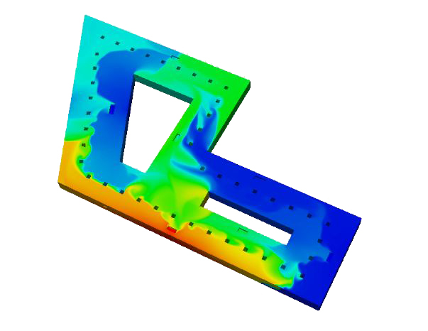
Figure 2: Smoke propagation inside a garage due to internal ventilation system
On the other side, explicit boundary conditions are needed when the injection of a chemical component in a region is simulated, e.g. a chimney stack (figure 3); in this case, a boundary condition on the inlet boundary is needed to be imposed (for instance c=1, if pure smoke is emitted into the atmosphere from the chimney or c=0.5 if the chimney output is a mixture of 50% smoke and 50% air).
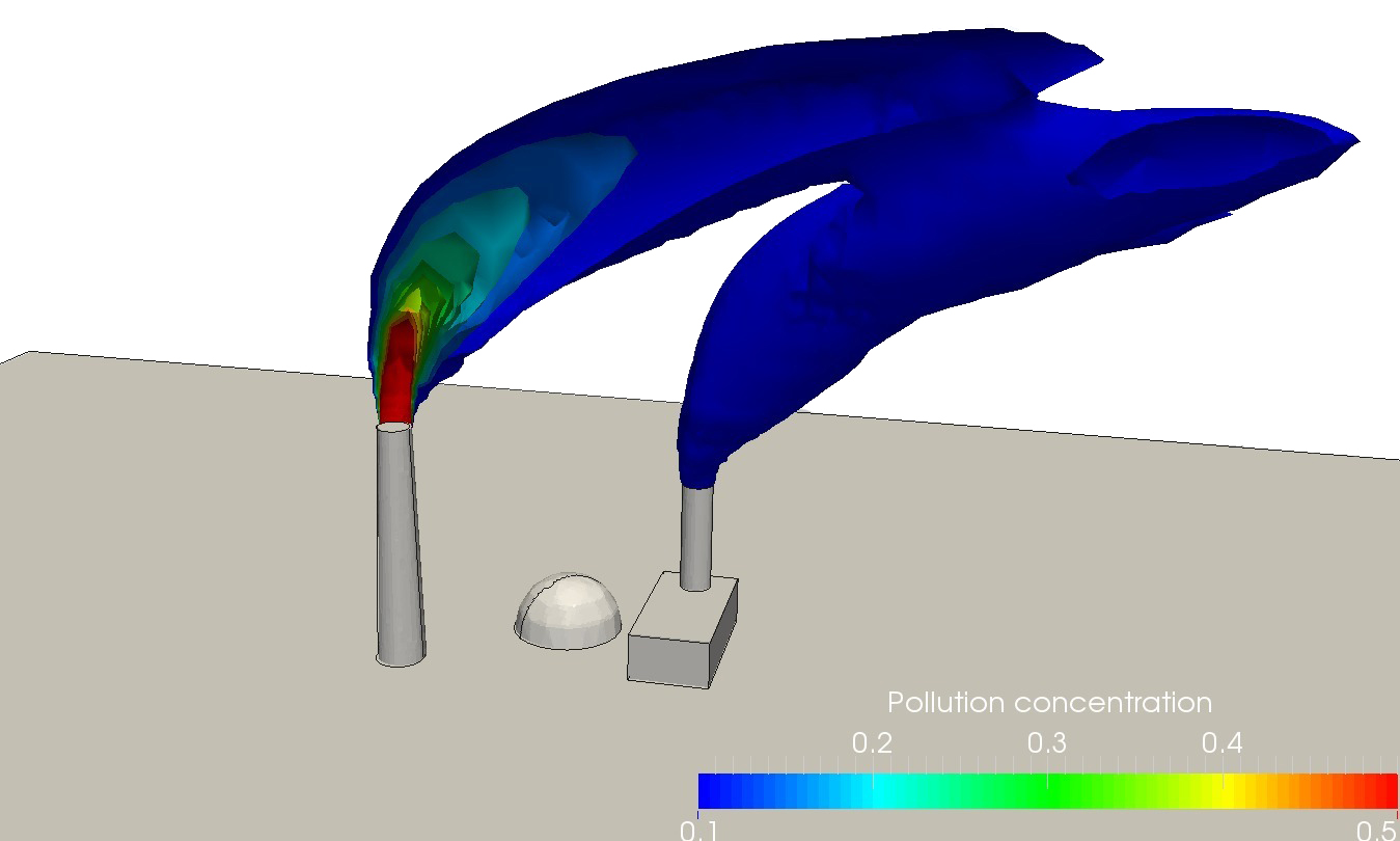
Figure 3: Smoke dispersion in the atmosphere due to two chimney stacks
Level-set method
The level set is a particular family of transportation models in which a distance function (named level-set function) is transported ^{2,3}. This distance function is computed with respect to an interface (surface for 3D problems, line for 2D problems, and point for 1D problems) and must have 2 characteristics:
- it must be an eulerian function, i.e. ||\nabla\varphi||=1 where \varphi is the level-set function
- it is signed, so it is positive on one side of the interface and negative on the other side.
For the sake of clarity, examples of the 1D and 2D distance function to be transported are shown in figure 4 and figure 5 respectively.
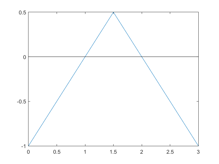
Figure 4: Level-set function computed in an 1D domain with respect to the interface \Gamma= [ x=1\cup x=2 ] .
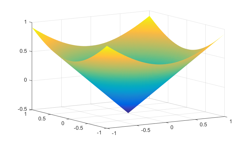
Figure 5: Level-set function computed in a 2D domain with respect to a circular interface with center C=(0,0) and radius r=0.5.
Level-set methods follow the principles of the classic transport equation, but they require a further computation step (called re-initialization) in order to maintain the Eulerian distance function condition. The main advantage of the use of a level-set function is the possibility to solve the transport equation just once, but to obtain many results in the post-processing. For instance, for multiphase flows (see the following section), it is possible to compute the transported viscosity and density fields, the surface tension, and to impose a mixing law across the interface with very little computational effort. In addition, the use of the level-set function allows dealing with fields which show high gradients (e.g. the density field for the simulation of a water droplet falling through the air). The transport of the density field would lead to numerical instabilities across the interface, where the density gradient is very high, while the transport of the level-set is more stable and enables computing the density as post-processing.
The transportation of a distance function has several engineering applications; in the following sections, we will report the most common ones.
Image segmentation
The purpose of level-set methods in image processing is to identify and export the contour of a certain profile in the image. This process (called image segmentation) is widely used in computer graphics and medical applications$^4$. It is commonly used to analyze ultrasounds and tomographies’ outputs in the localization of tumors; in figure 6 it is shown the segmentation process for an ultrasound of lungs. By the segmentation process, it is possible to identify objects inside a digital image (i.e. the lungs) through the identification of its boundaries and, eventually, use this information for the analysis of the pathology.
Figure 6: Image segmentation of a lungs tomography$^{5}$.
In the case of image segmentation, convection and source terms in equation 3 are not considered; the only means of transport is diffusion according to the gradient of pixels density of the image.
Multiphase flow
The level-set method is also commonly used to simulate multiphase flows. In this case, the transport model is defined as “active transport” because convection/diffusion of the interface (through the distance function) affects the flow. The distance from the interface influences the flows because it is used to compute the material parameters in the computational domain; given a flow composed by two fluids characterized by different material properties \eta_1 and \eta_2, the value in any given position (or element, in the case of numerical simulation) is given by:
where H(\phi) is the Heaviside function defined as
In this way, any complex multiphase flow with non-uniform material properties can be modeled through the simple transport of a scalar field (the level-set function) and the interface can be tracked implicitly as the zero Isocontour of this function. In figure 7, the results of the simulation of a rising bubble are shown; in this case, the interface represents the \varphi=0 isoline, while the region where \varphi>0 is colored in blue and the region where \varphi<0 is colored in red.
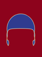
Figure 7: Rising air bubble in a liquid domain
Microstructure analysis
Similarly to the simulation of multiphase flows, the level-set method is used for the modelling of material crystallization. The transport of the level-set function is the starting point to analyze the phase change and crystals growth within a material. In figure 8, an example of a 2D representation of the crystal structure of a material through level-set method is presented: each microstructural grain is identified through its boundaries (the zero-level of the level-set function), while the color is based on the level-set function in order to distinguish the grain.
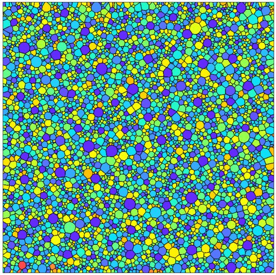
Fig. 8: 2D polycrystal containing 5000 grains representative of a 304L austenitic steel$^{6}$
Related Topics
Resources
^1: https://www.io-warnemuende.de/tl_files/project/amber/workshops/Lagoon%20Ecosystem%20Modelling/SSK-Lecture4.pdf
^2: https://math.berkeley.edu/~sethian/Papers/sethian.vallambrosa.87.pdf
^3: https://math.berkeley.edu/~sethian/Papers/sethian.osher.88.pdf
^4: http://physbam.stanford.edu/~fedkiw/
^5: https://www.youtube.com/watch?v=1R9oJ4OrTD0
^6: http://chaire-digimu.cemef.mines-paristech.fr/wp-content/uploads/2017/01/ManuscrittheseScholtes.pdf
