Recording

Homework
Submitting all three homework assignments will qualify you for a free Professional Training (value of 500€) as well as a certificate of participation.
Homework 3 - Deadline 30.06 12:00pm
Please use the form to submit your homework
Exercise
The aim of this exercise it to investigate two different cooling concepts for a Raspberry-Pi housing.
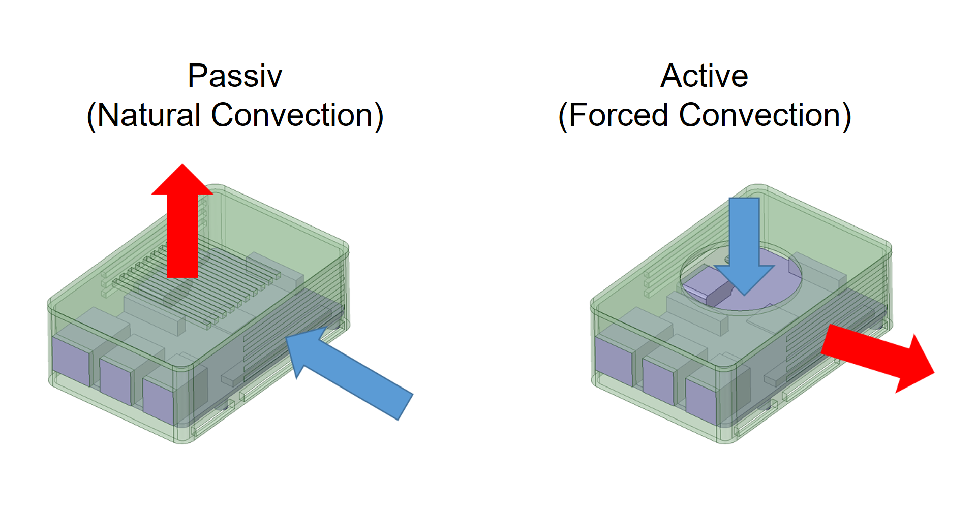
The two variants differ in terms of their underlying heat transfer mechanisms:
The passive design has only ventilation slots on top of the housing and the housing flank. Due to the heat transfer from the hot plate to the cool air, the heat rises and exits the housing through the upper slots. This gives rise to a subsequent flow of fresh cooling air through the slits on the side.
In contrast, the ‘active’ design has a fan on top of the case. This “forces” air flow through the housing.
Step-by-Step Instructions
NOTE: This tutorial was updated on 10/2016 to match the updated version of the platform
Meshing
First of all, you have to import the geometry into your SimScale workspace. For this, you only have to click on this link.
Please note that this can take several minutes.
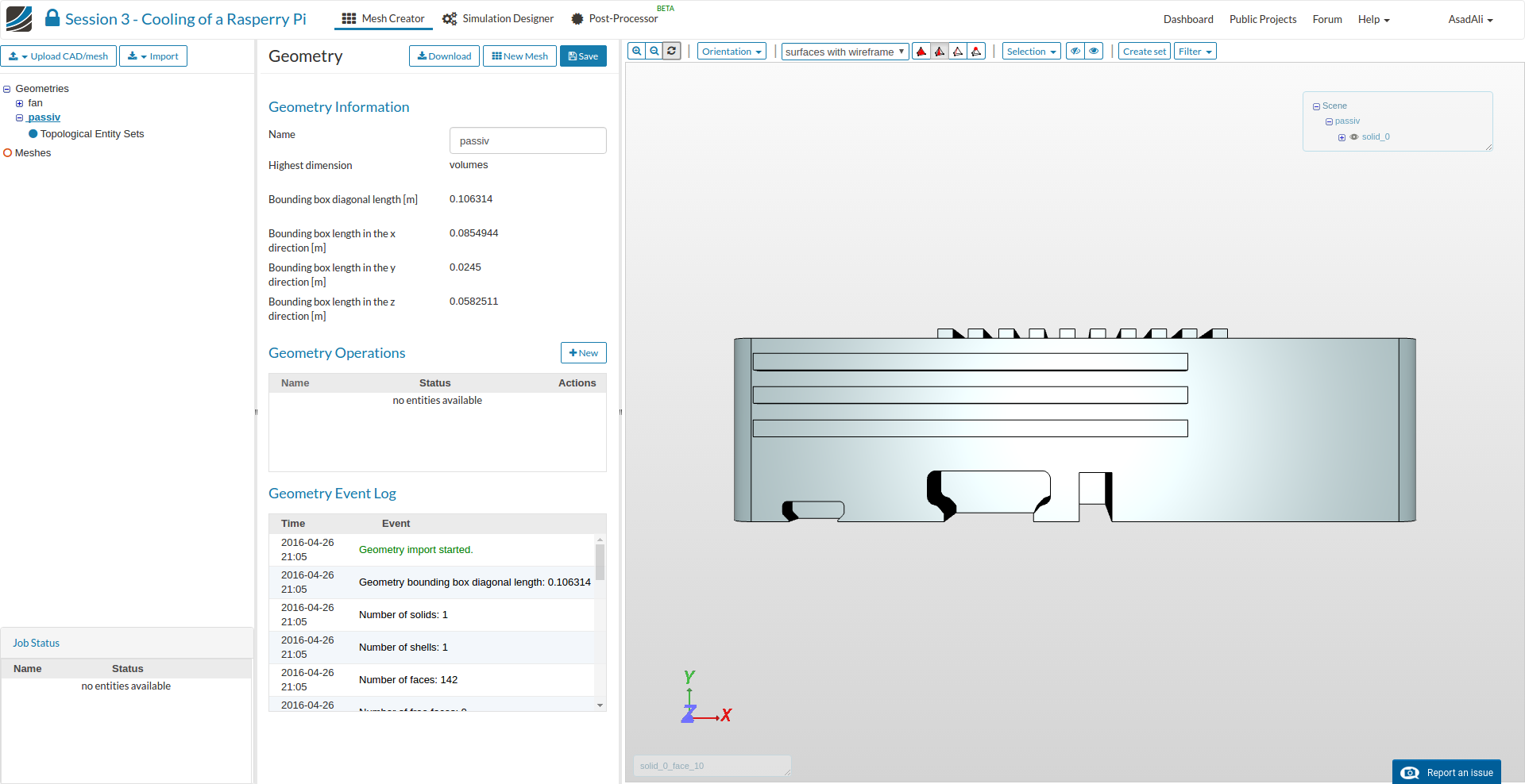
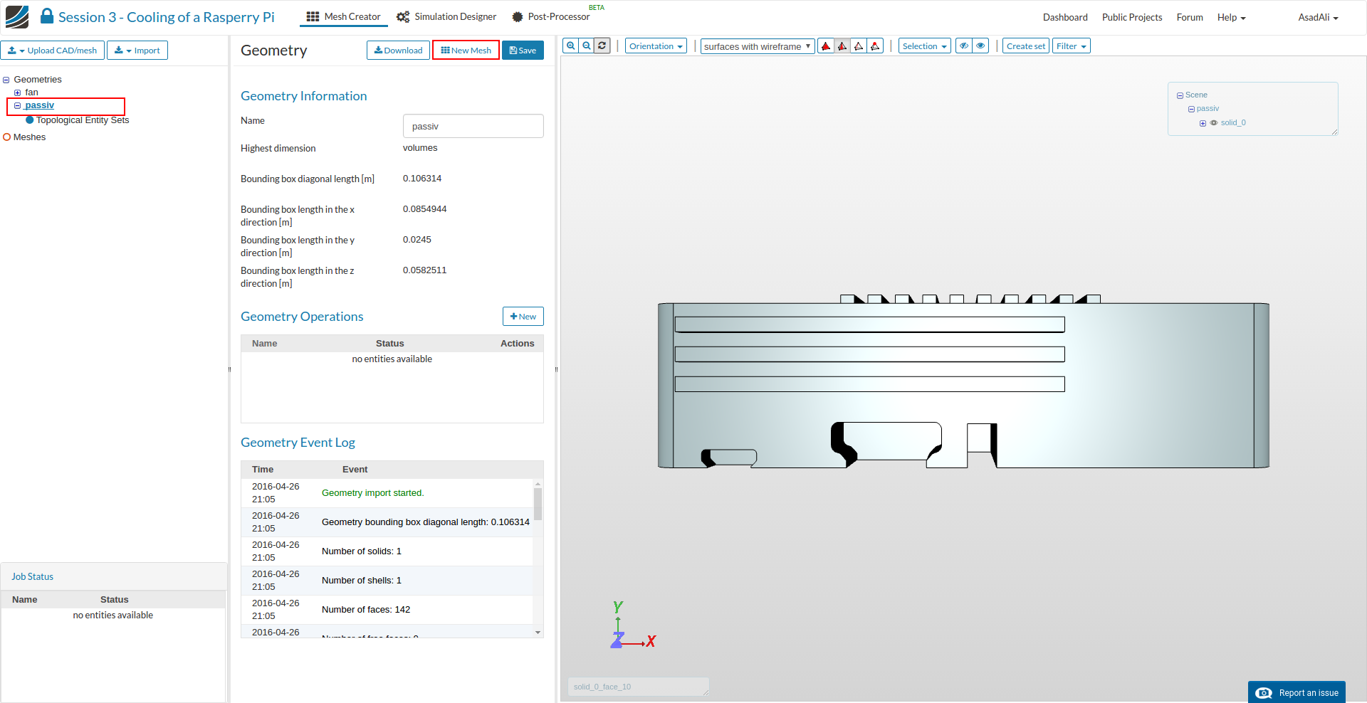
Now, select the geometry you want to mesh, in this case first we will mesh “passiv” model, and click on the New Mesh item in the middle column.
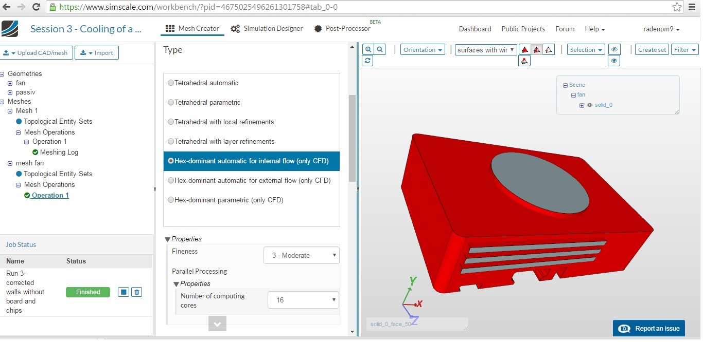
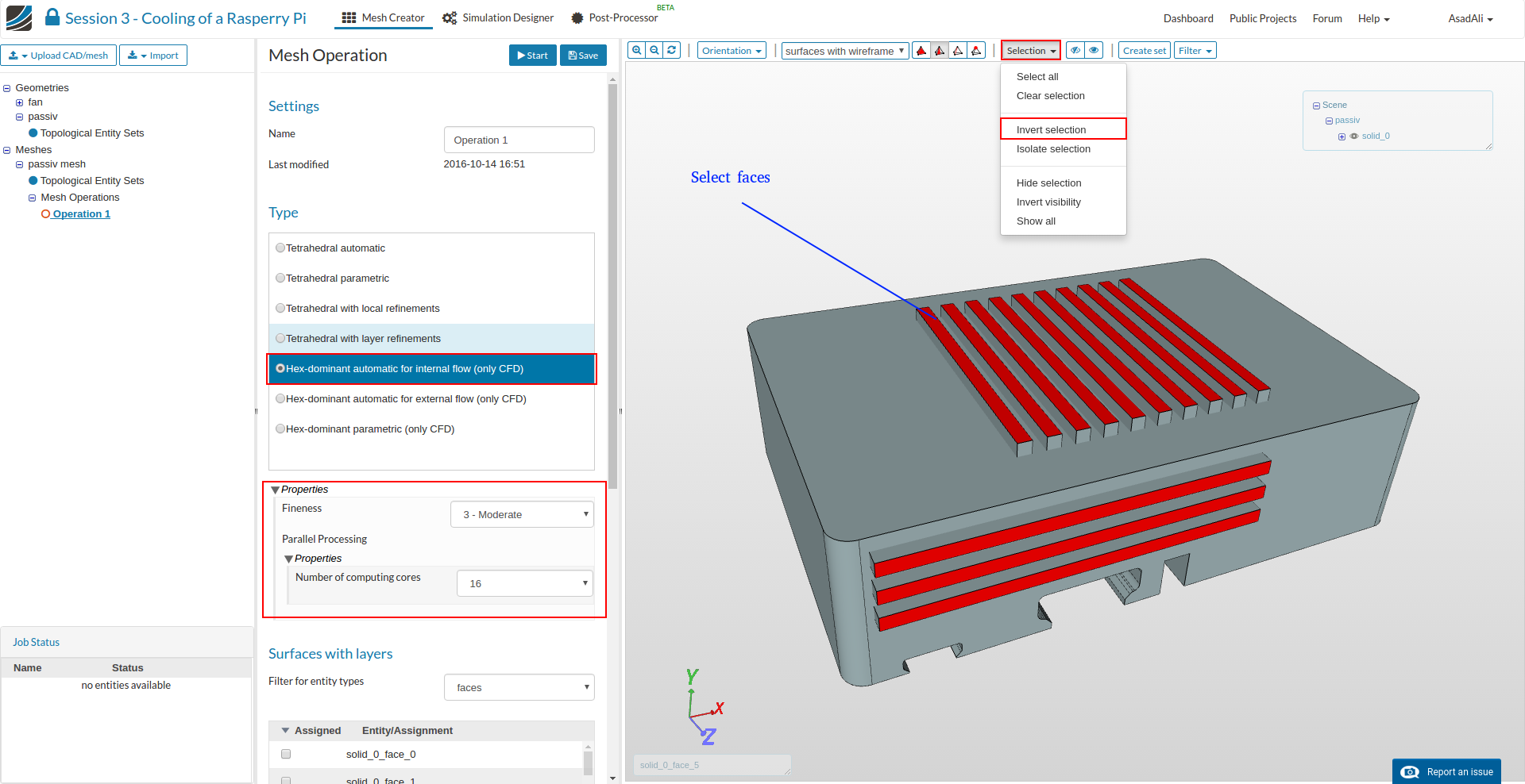
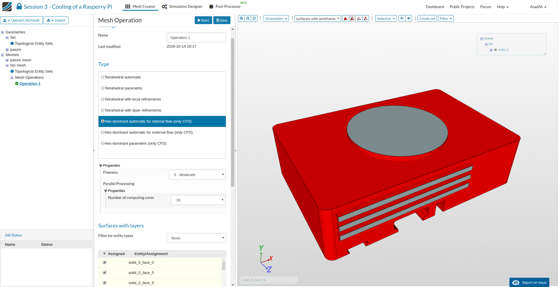
This will open an additional column in the middle. Here you can set the parameters for the meshing. Select Hex-dominant automatic for internal flow (only CFD) from the list and adapt following parameters:
- Fineness: 3 - Moderate
- Number of computing cores: 16
This meshing operation will automatically create a mesh for fluid flow simulation. The cell size and refinement will be adapted automatically.
In addition, we want to create a prism layer near the walls . This is characterized by very flat elements that are able to resolve the boundary layer appropriately. However, these should not be created on the inlet or outlet , as these areas do not have any boundary layer .
It is recommended to first select the inlet and outlet graphically and to invert your selection afterwards by clicking the related button.
Then just click on the Add selection from viewer button to add the faces you’ve selected before. Now click on the Start button to start meshing.
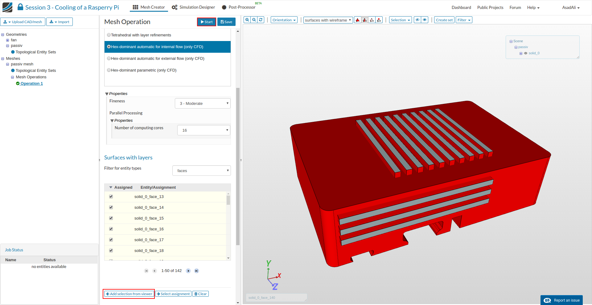
The meshing process will take few minutes to finish.
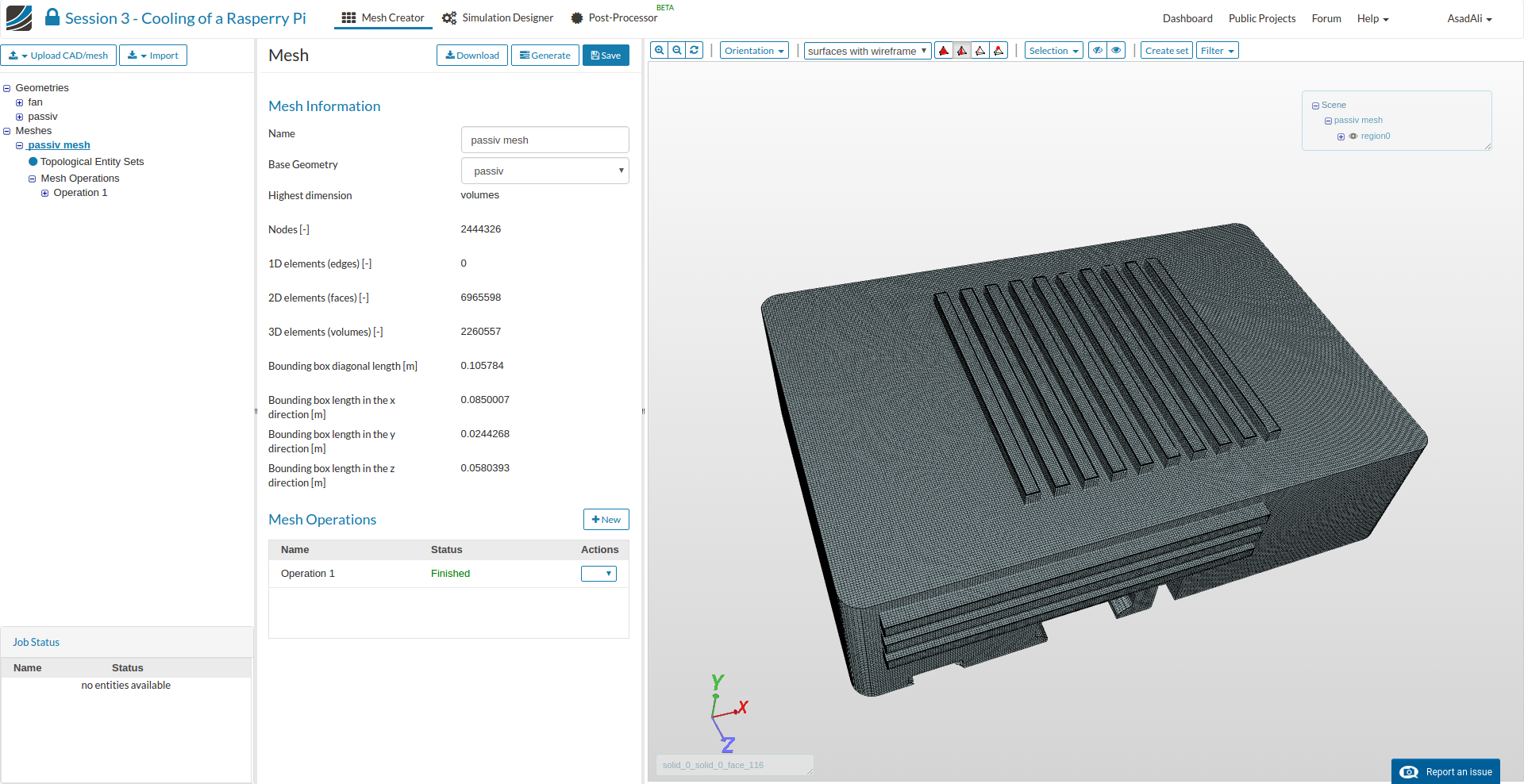
Simulation Setup
Once mesh is finished, move to the Simulation Designer tab and click on the New button to create a simulation run.
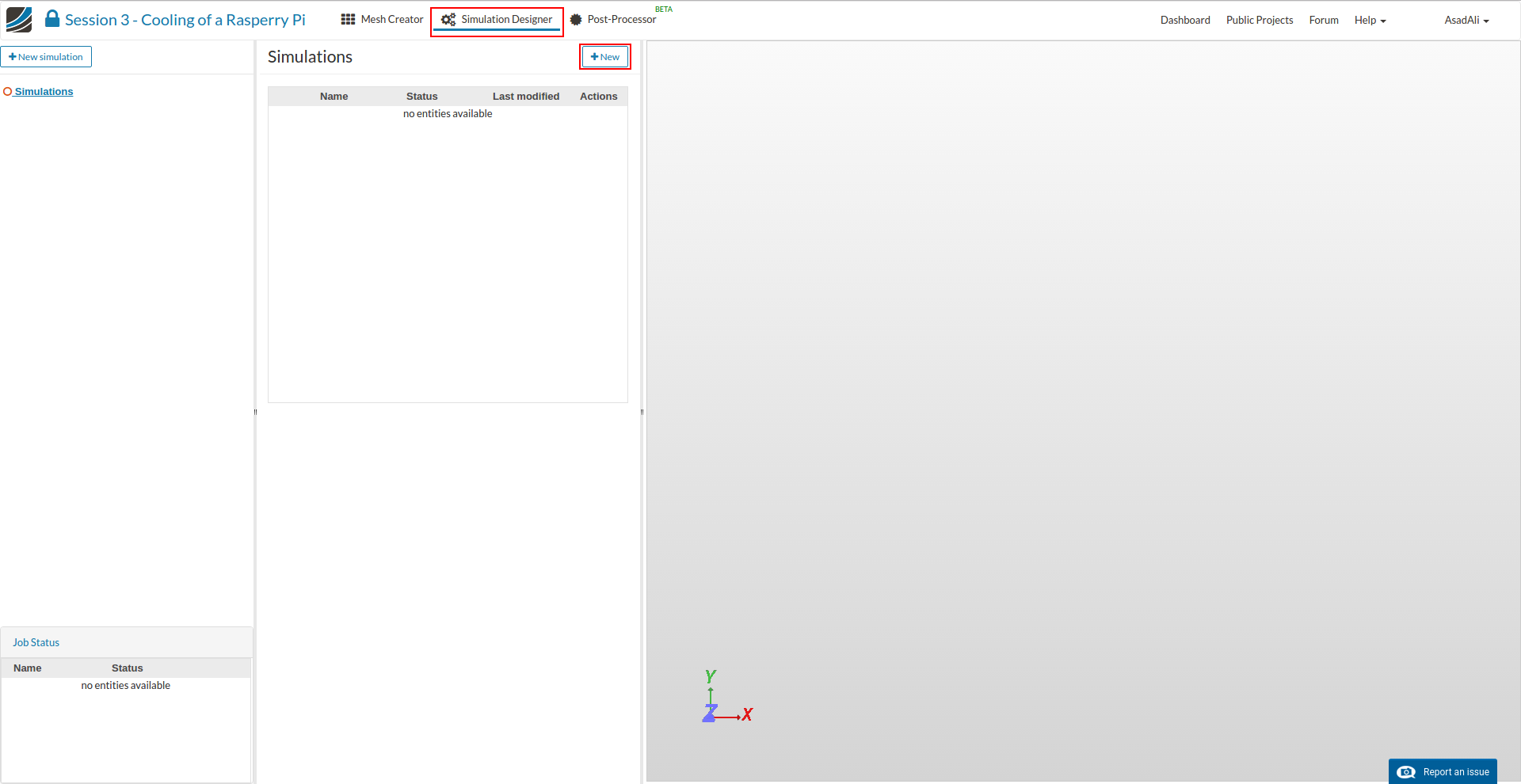
This will open an additional column in the middle. Here you can select which kind of simulation you want to run.
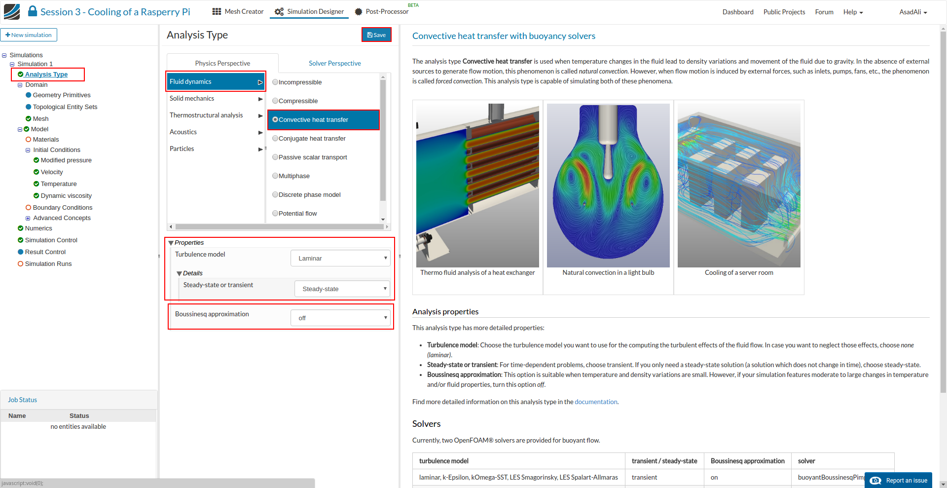
In our case we will run a Fluid dynamics simulation of Convective heat transfer.
Now you can define some additional settings. First of all choose Laminar as the turbulence model, since we are not expecting any turbulence. Then choose Steady-State from the drop down field below. This means that we will simulate the stationary flow field. choose “off” for Boussinesq approximation since its mostly used for liquids. Finally, save your settings by clicking the related button at the bottom, which will create additional items in the project tree on the left side.
Next you have to specify which mesh you want to use for your simulation. Click on Domain item in the project tree and select passiv mesh from the menu which disappears in the middle column. Don’t forget to save your selection.

Next we have to define the physical Model we want to use for this simulation. Click on the Model item in the project tree which will open a middle column windows. Here you can define the gravitation.
- x value: 0
- y value: -9.81
- z value: 0

Now we have to specify the material properties of the fluid by defining the kinematic viscosity. Therefore click on the Materials sub-item in the project tree.
Click on the New button.

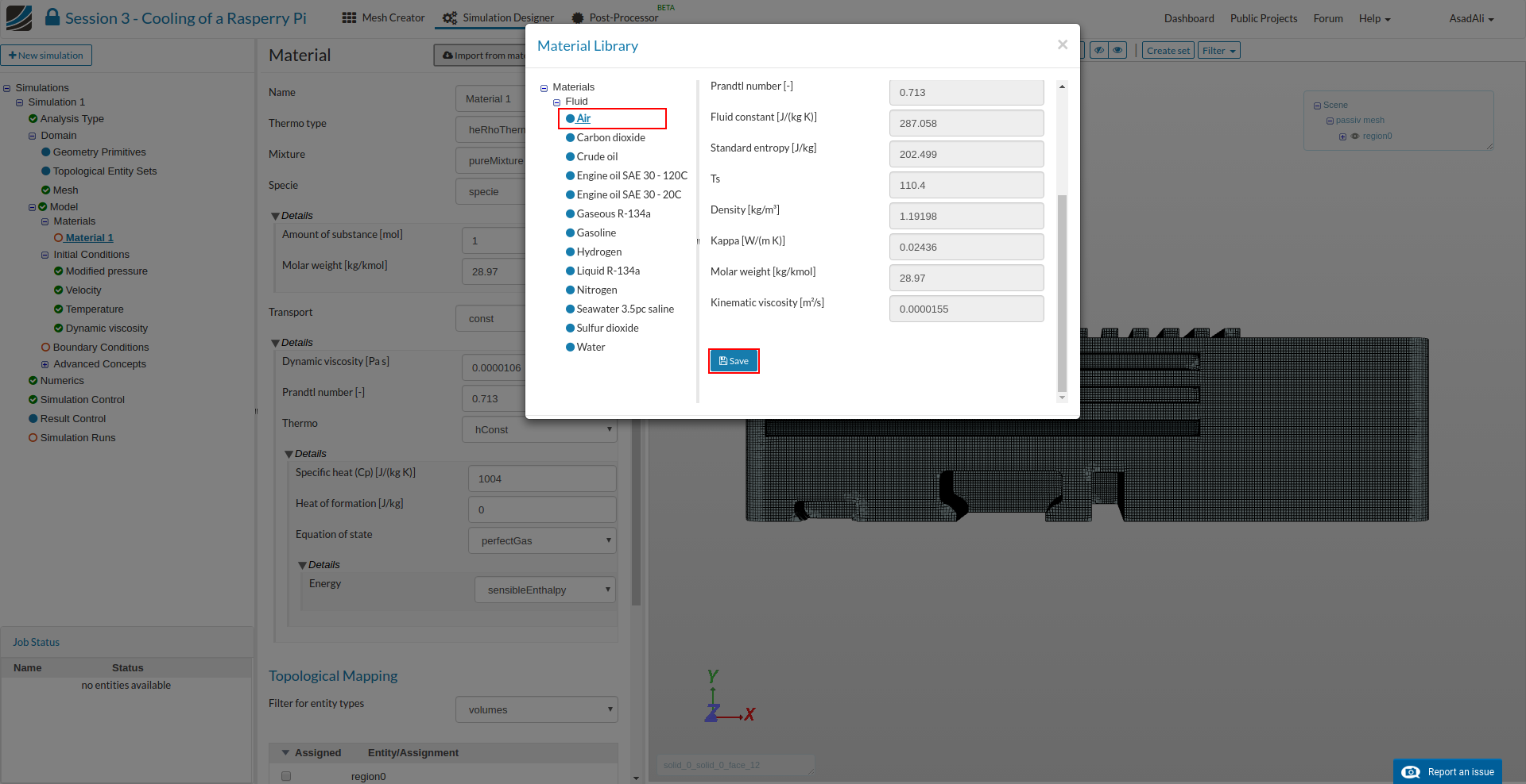
This will open a new middle column windows where you can assign fluids to your mesh. SimScale also comes with a material library which we will use. Click on the Import from material library button. Here choose Air from the list on the left side and save your selection.
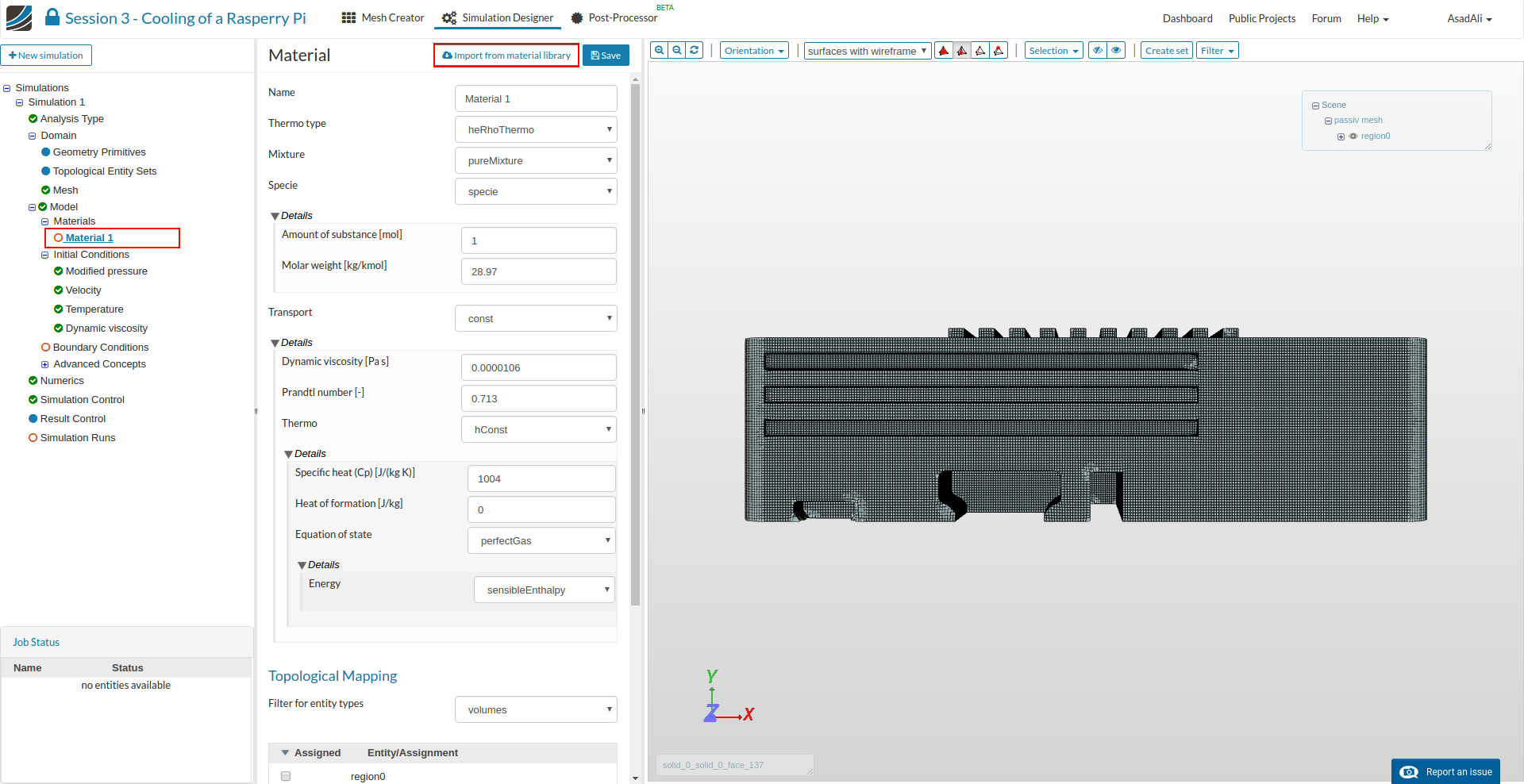
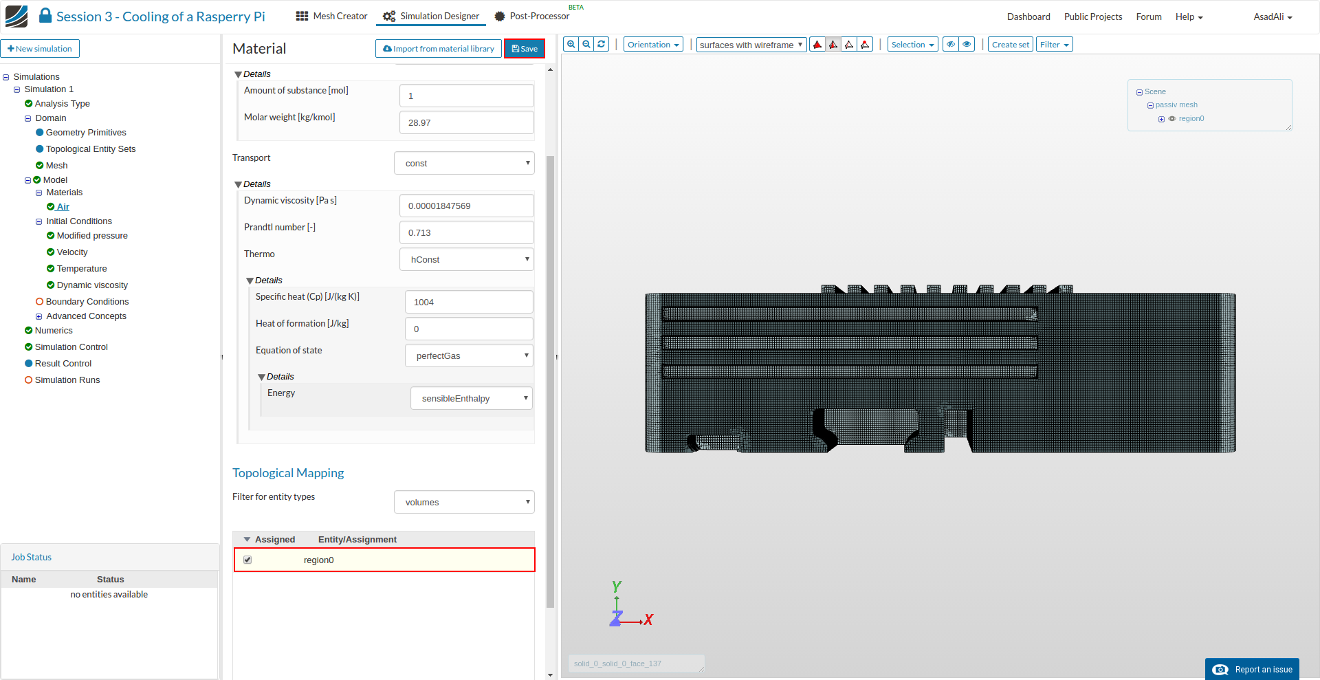
Finally, we have to assign which parts of the mesh should be from this material. Please assign the material model to your mesh (region0)
Now we have to assign Initial Conditions and Boundary Conditions
The initial conditions are used as a starting solution for the calculation . Here you should to keep in mind that simulation result can be calculated approximately only. The applied numerical method operates in a loop.
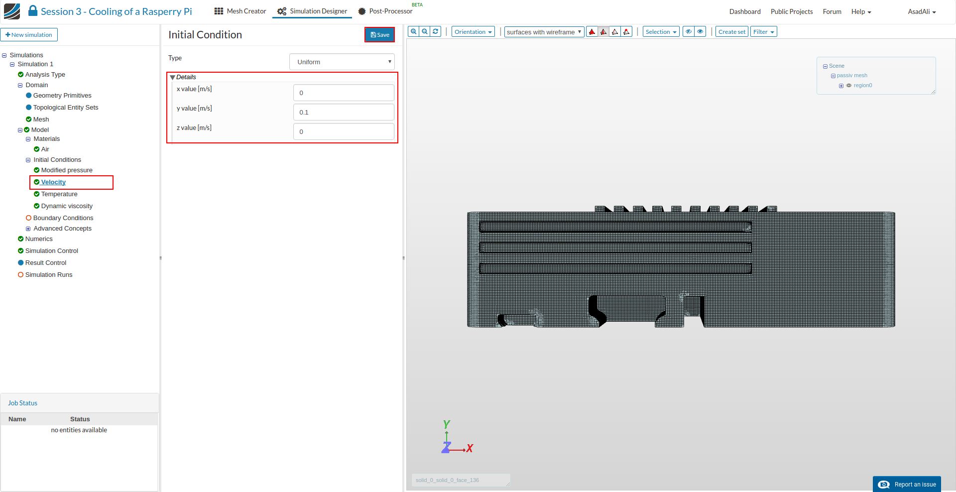
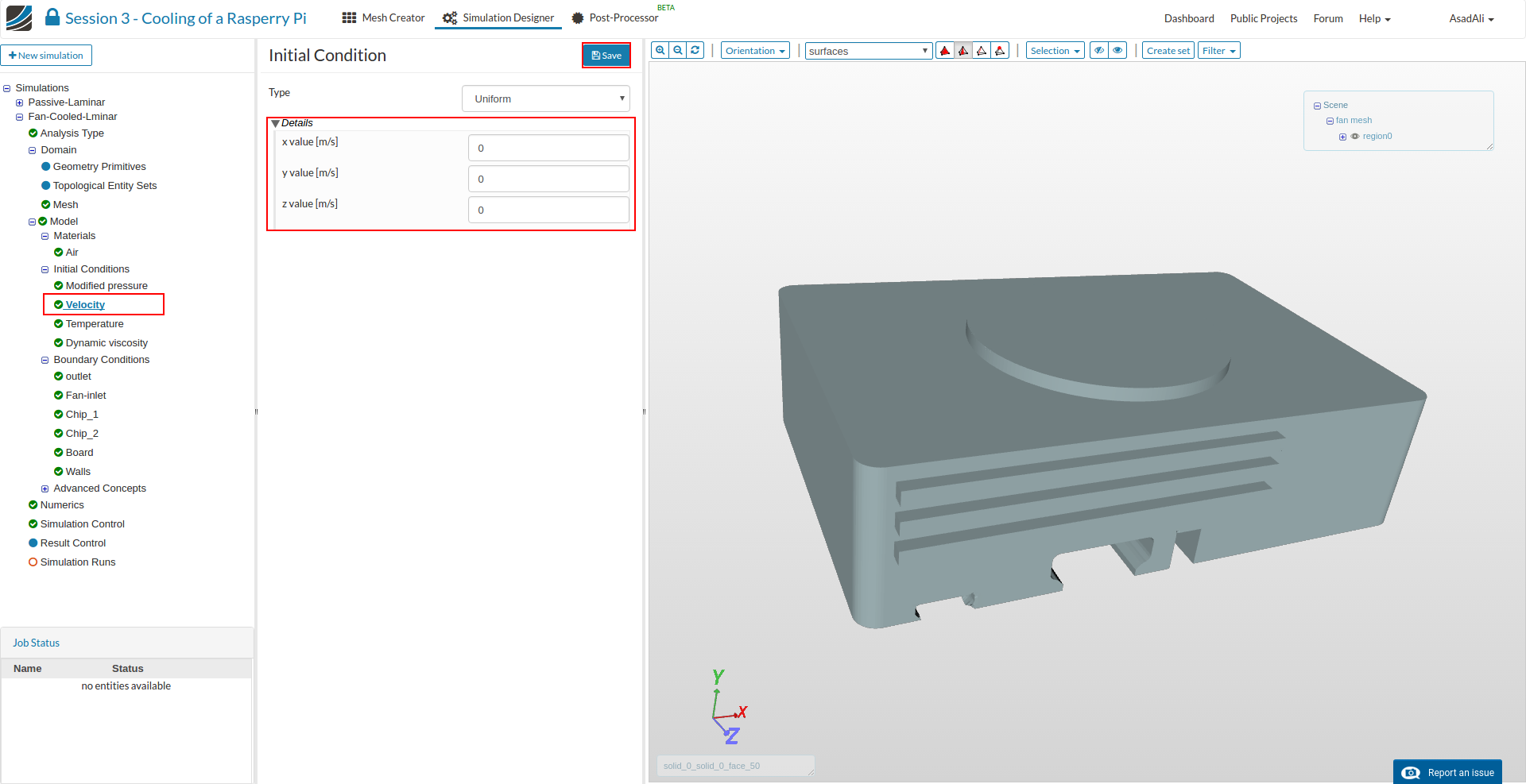
For our simulation, we need only to adapt the initial conditions for speed and viscosity:
Velocity
- x value [m/s] = 0
- y value [m/s] = 0.1
- z value [m/s] = 0
Dynamic viscosity
- Dynamic viscosity value = 0.0000155

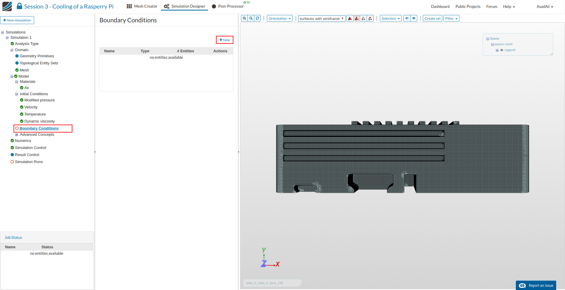
Boundary Conditions describe the interaction between your model and it’s environment.
Please click on the Boundary Conditions element to create new boundary conditions or modify existing ones. Click on the Add boundary condition button.
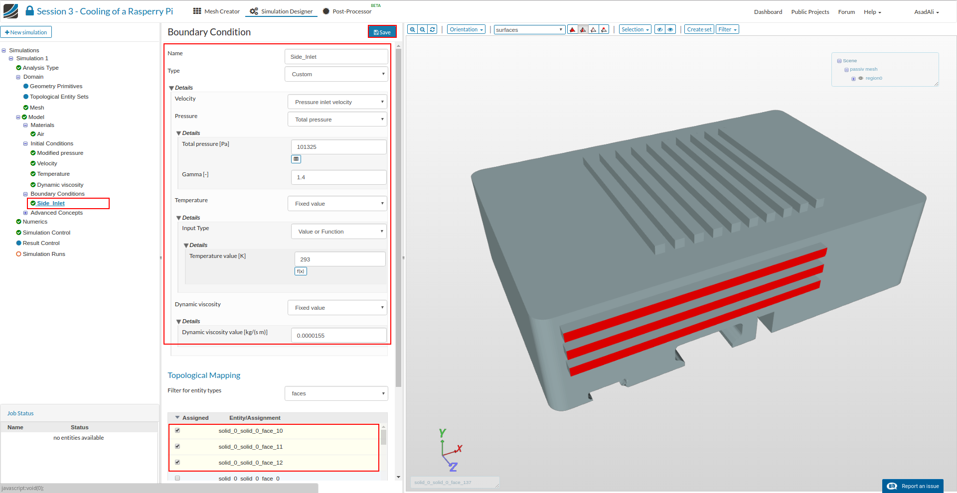
Side_Inlet
Since warm air rises, we can assume that by the lateral louvers only air enters but does not come out.
- Name: Side_Inlet
- Type: Custom
- Velocity: Pressure inlet velocity
- Pressure: Total pressure
- Total pressure [Pa]: 101325
- Gamma [-]: 1.4
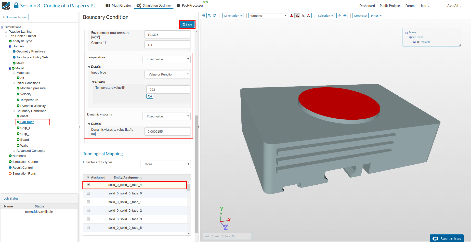
- Temperature: Fixed value
- Temperature value [k]: 293
- Dynamic viscosity: Fixed value
- Dynamic viscosity value [kg/(s/m)]: 0.0000155
Please assign following faces to your boundary condition (graphically or selection via list):
solid_0_solid_0_face_10, solid_0_solid_0_face_11, solid_0_solid_0_face_12
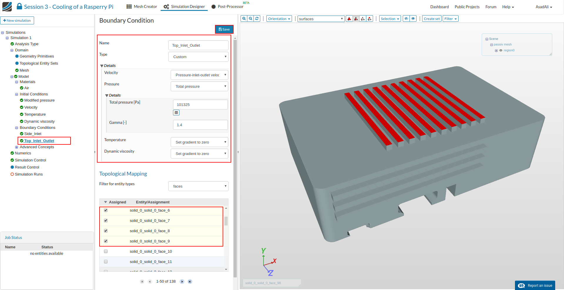
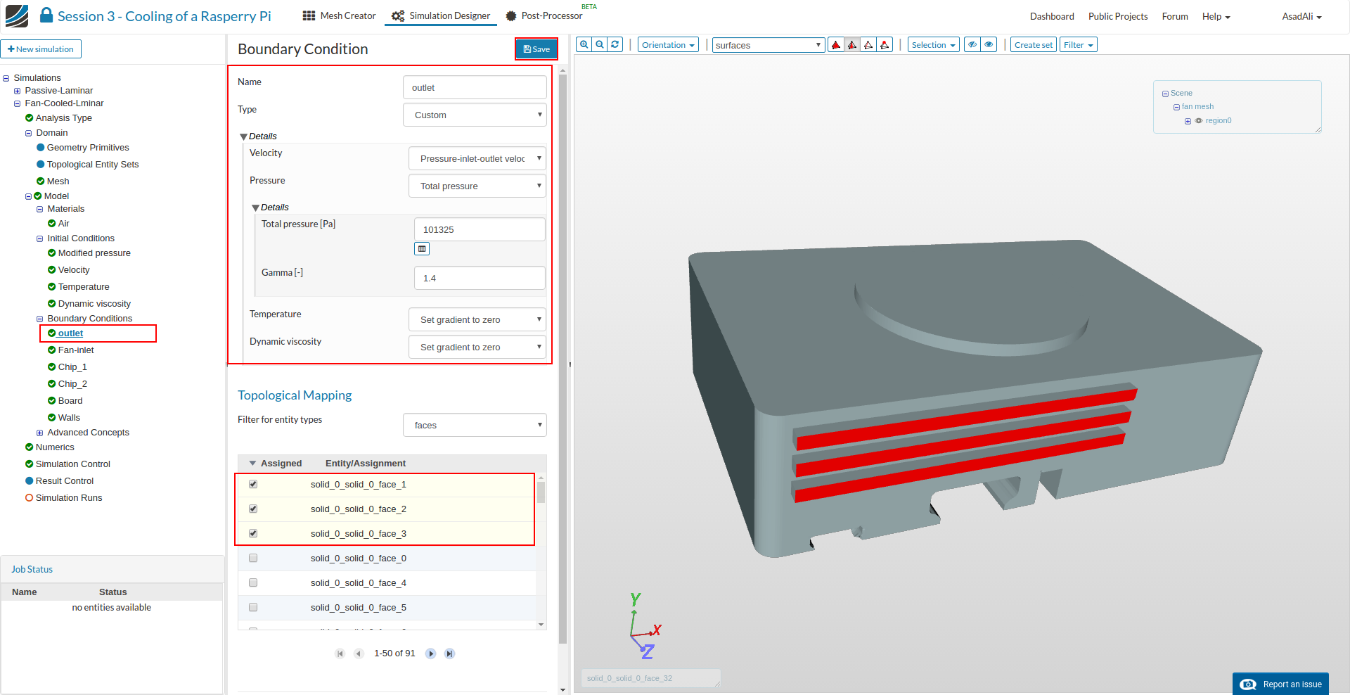
Top_Inlet_Outlet
*For the airflow through the upper cooling slots, we can not assume the flow direction.
- Name: Top_Inlet_Outlet
- Type: Custom
- Velocity: Pressure inlet-outlet velocity
- Pressure: Total pressure
- Total pressure [Pa]: 101325
- Gamma [-]: 1.4
- Temperature: set gradient to zero
- Dynamic viscosity: set gradient to zero
Please assign following faces to your boundary condition (graphically or selection via list):
solid_0_solid_0_face_0, solid_0_solid_0_face_1, solid_0_solid_0_face_2, solid_0_solid_0_face_3, solid_0_solid_0_face_4, solid_0_solid_0_face_5, solid_0_solid_0_face_6, solid_0_solid_0_face_7, solid_0_solid_0_face_8, solid_0_solid_0_face_9
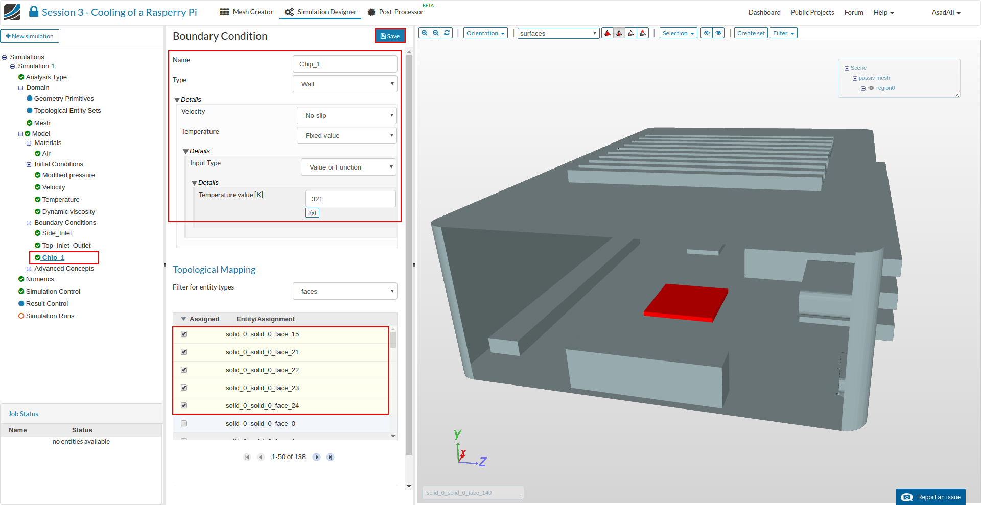
Chip_1
The surface temperature was measured with an IR camera
- Name: Chip_1
- Type: Wall
- Velocity: No-slip
- Temperature: Fixed value
- Temperature value [k]: 321
Please assign following faces to your boundary condition (grapically or selection via list):
solid_0_solid_0_face_15, solid_0_solid_0_face_21, solid_0_solid_0_face_22, solid_0_solid_0_face_23, solid_0_solid_0_face_24
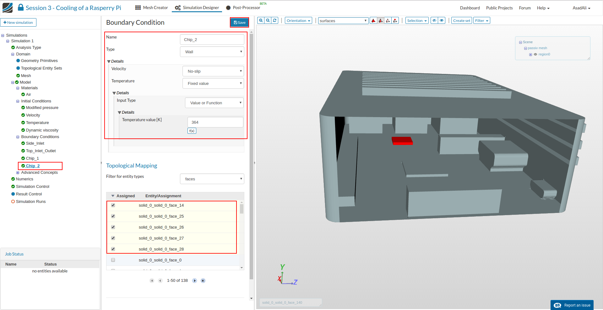
Chip_2
The surface temperature was measured with an IR camera
- Name: Chip_2
- Type: Wall
- Velocity: No-slip
- Temperature: Fixed value
- Temperature value [k]: 364
Please assign following faces to your boundary condition (grapically or selection via list):
solid_0_solid_0_face_14, solid_0_solid_0_face_25, solid_0_solid_0_face_26, solid_0_solid_0_face_26, solid_0_solid_0_face_28
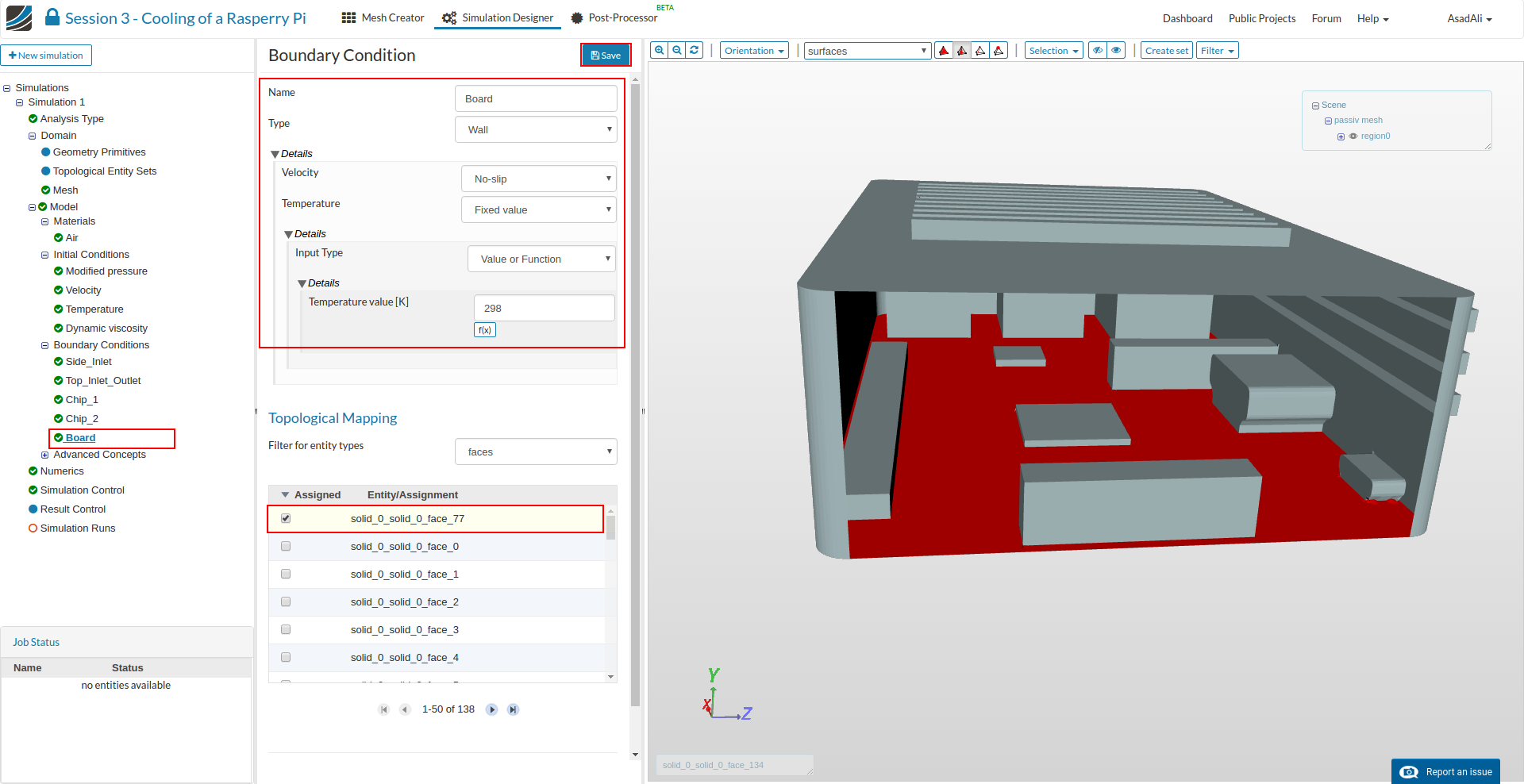
Board
The surface temperature was measured with an IR camera
- Name: Board
- Type: Wall
- Velocity: No-slip
- Temperature: Fixed value
- Temperature value [k]: 298
Please assign following faces to your boundary condition (grapically or selection via list):
solid_0_solid_0_face_77
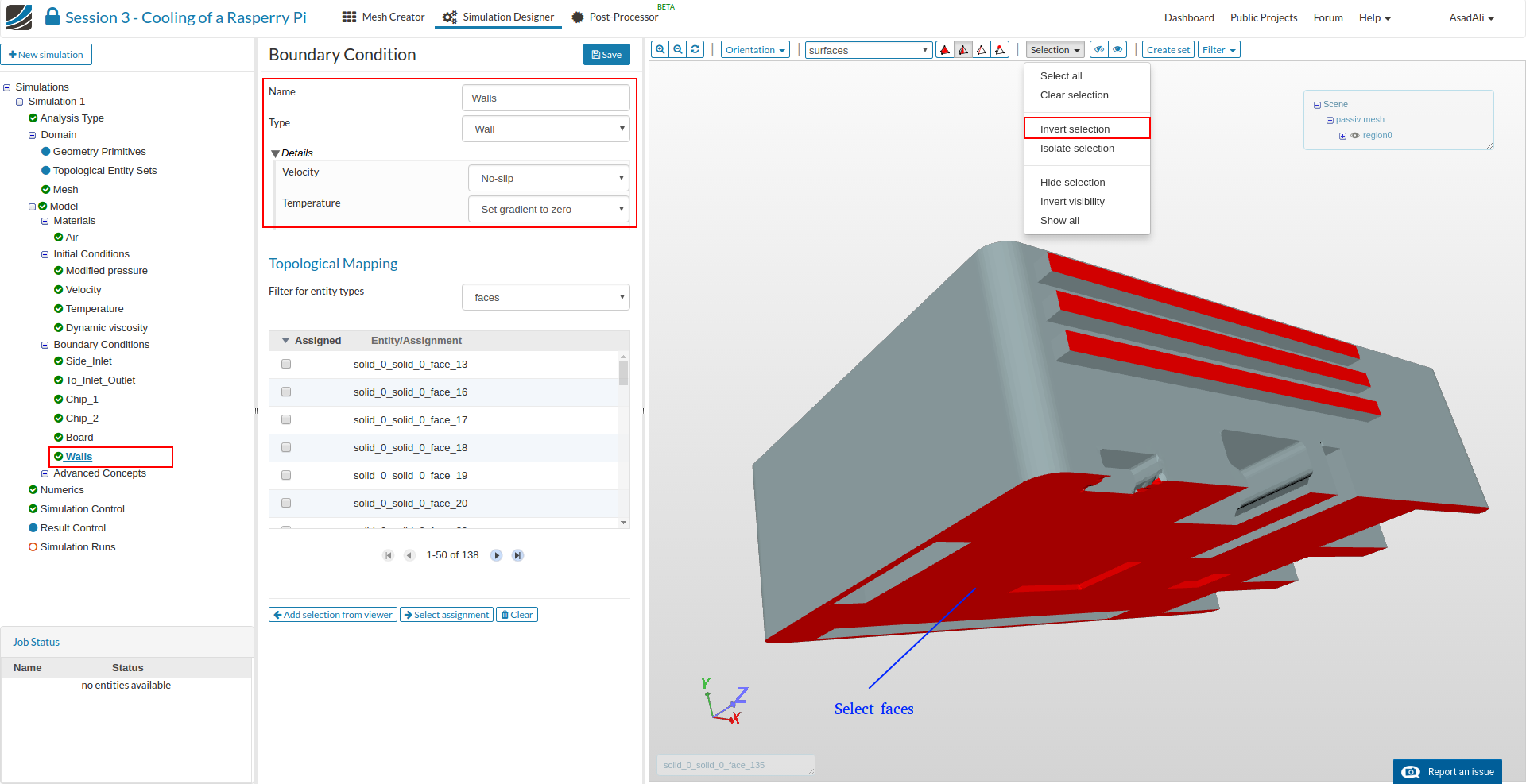
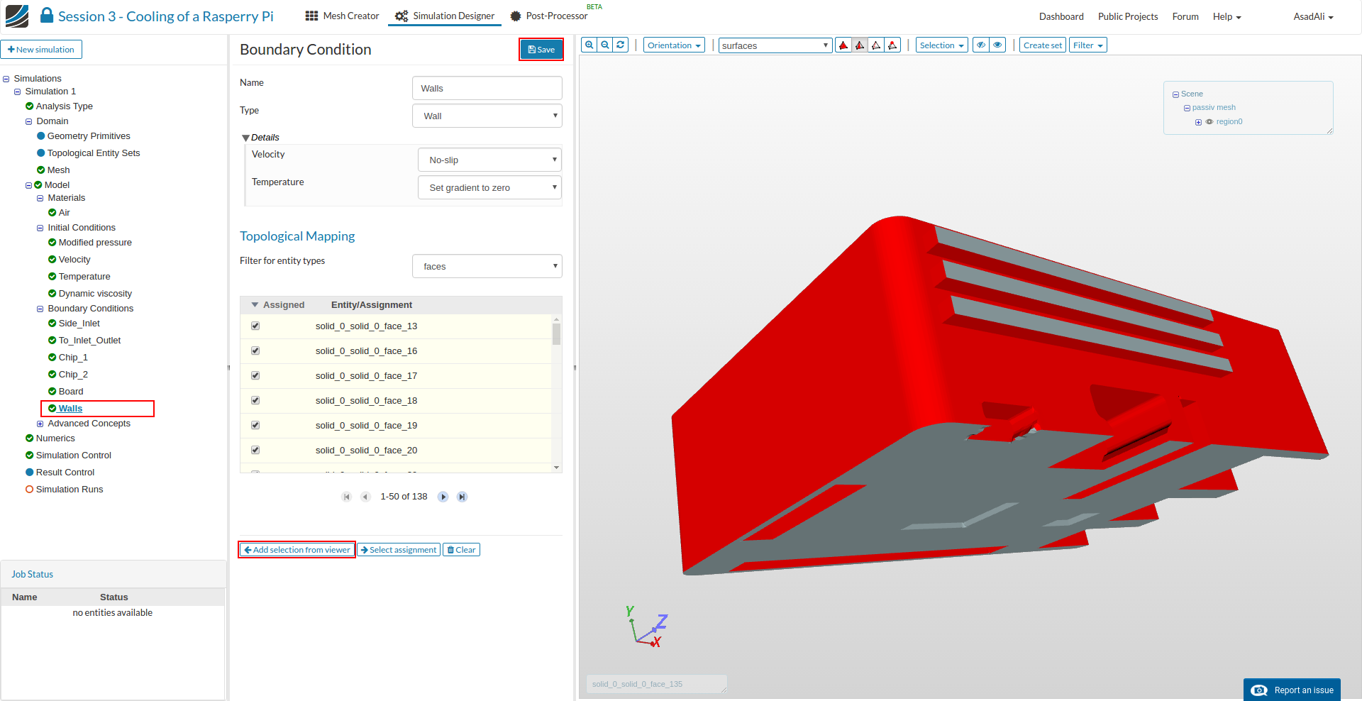
Walls
The temperature distribution of the other surfaces is not specified , since it is unknown. To simplify the selection of the related faces we recommend to use again the invert selection feature
- Name: Walls
- Type: Wall
- Velocity: No-slip
- Temperature: set gradient to zero
Please assign all remaining faces to this boundary condition
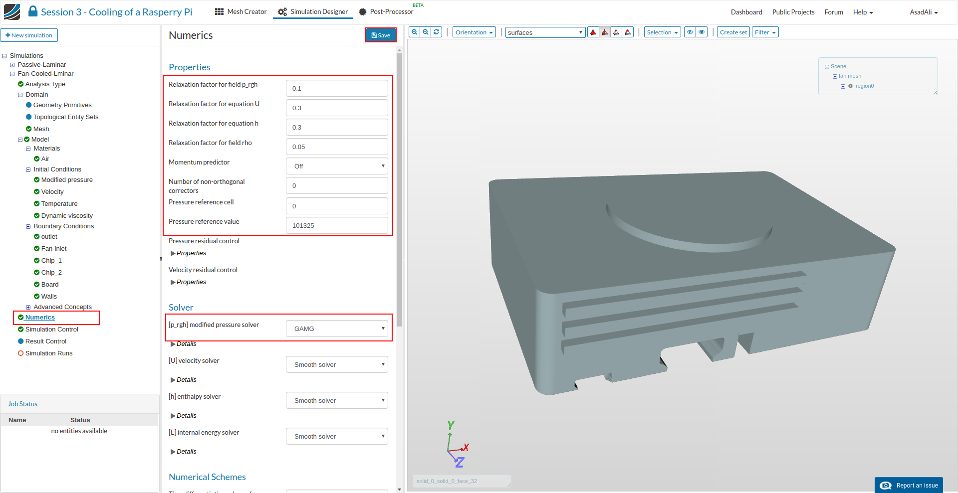
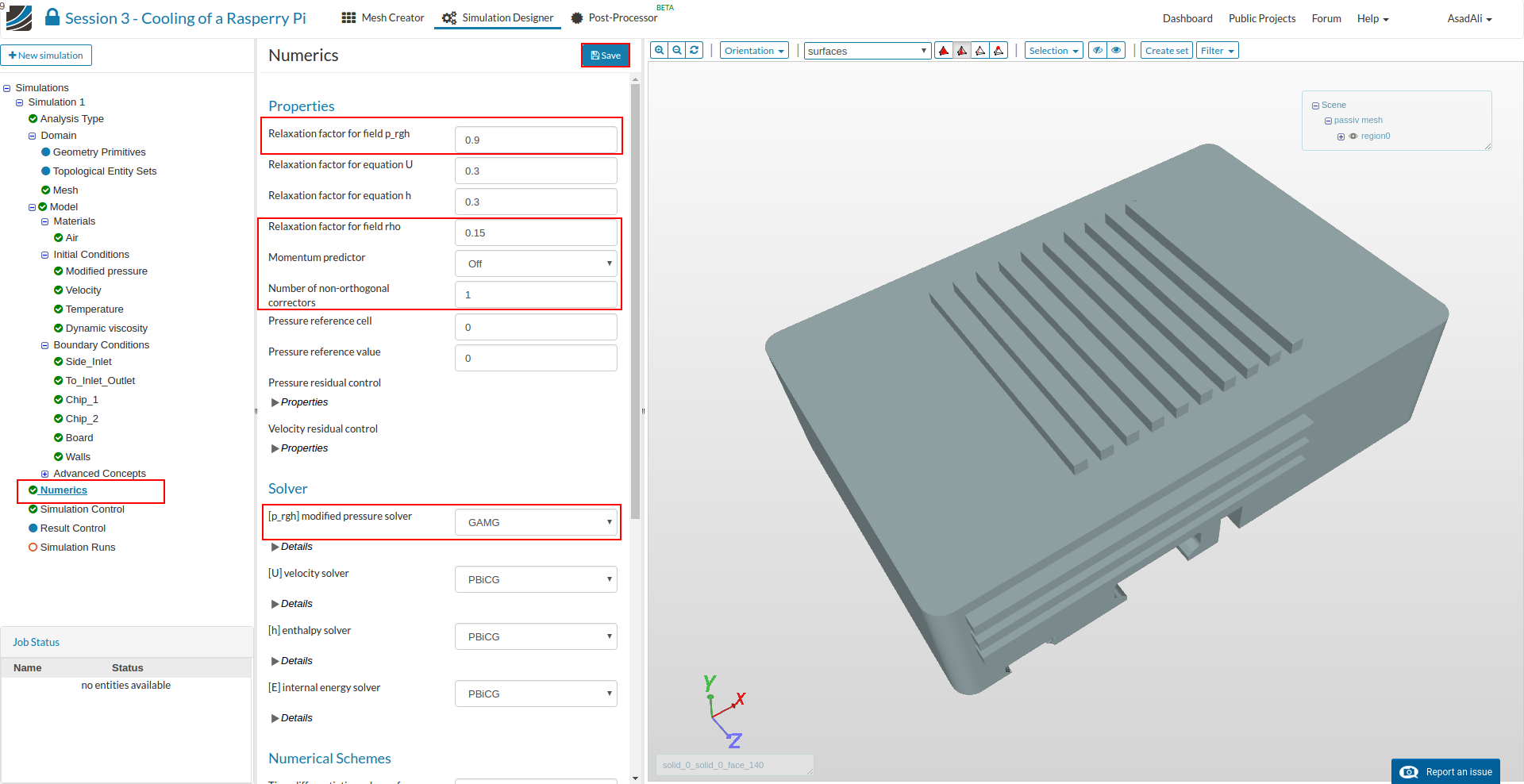
Now we have to modify some of the numerical settings. This is not absolutely necessary but it will help to reduce the simulation time and make it more stable. Click on the Numerics items in the tree and change the settings and values according to the image below (Please note that you may have scroll down).
Click on the Simulation Control item in the project tree to specify how fast and accurate you want the simulation to be computed.

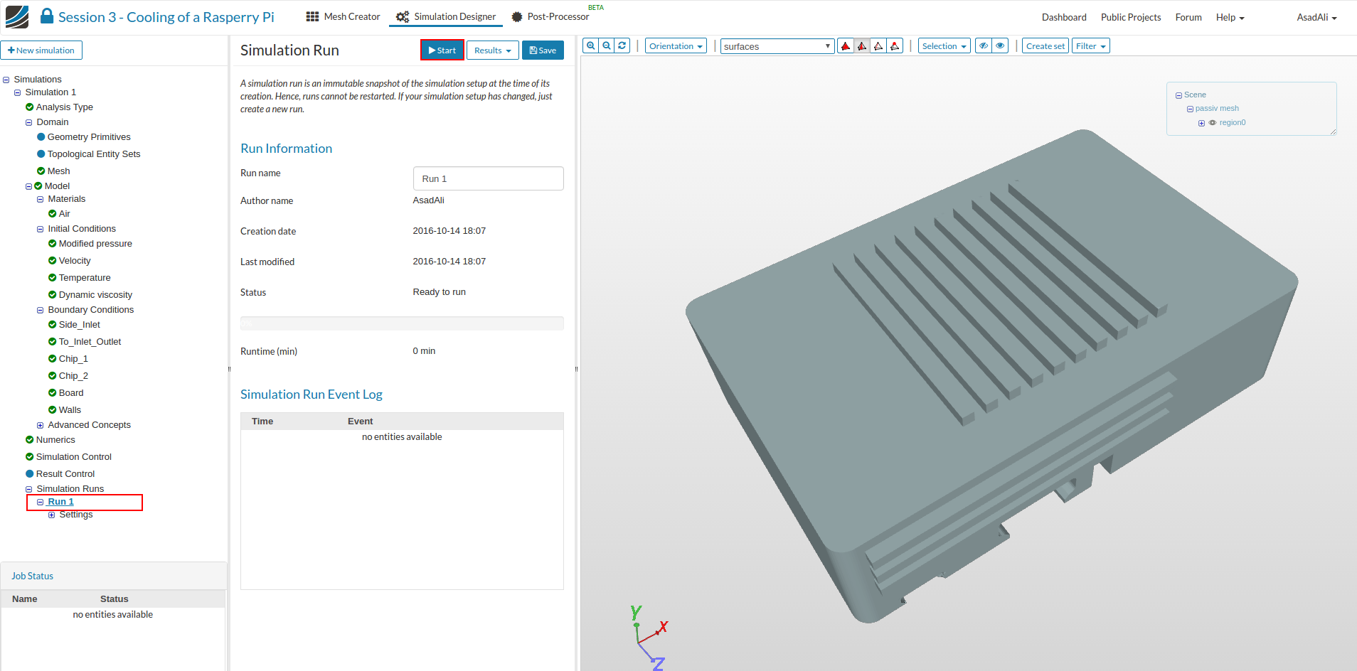
To start the simulation, click on the Simulation Run item in the tree and click on the Create new run button at the bottom of the middle column menu. This will create a snapshot of your simulation settings as a new sub-item.
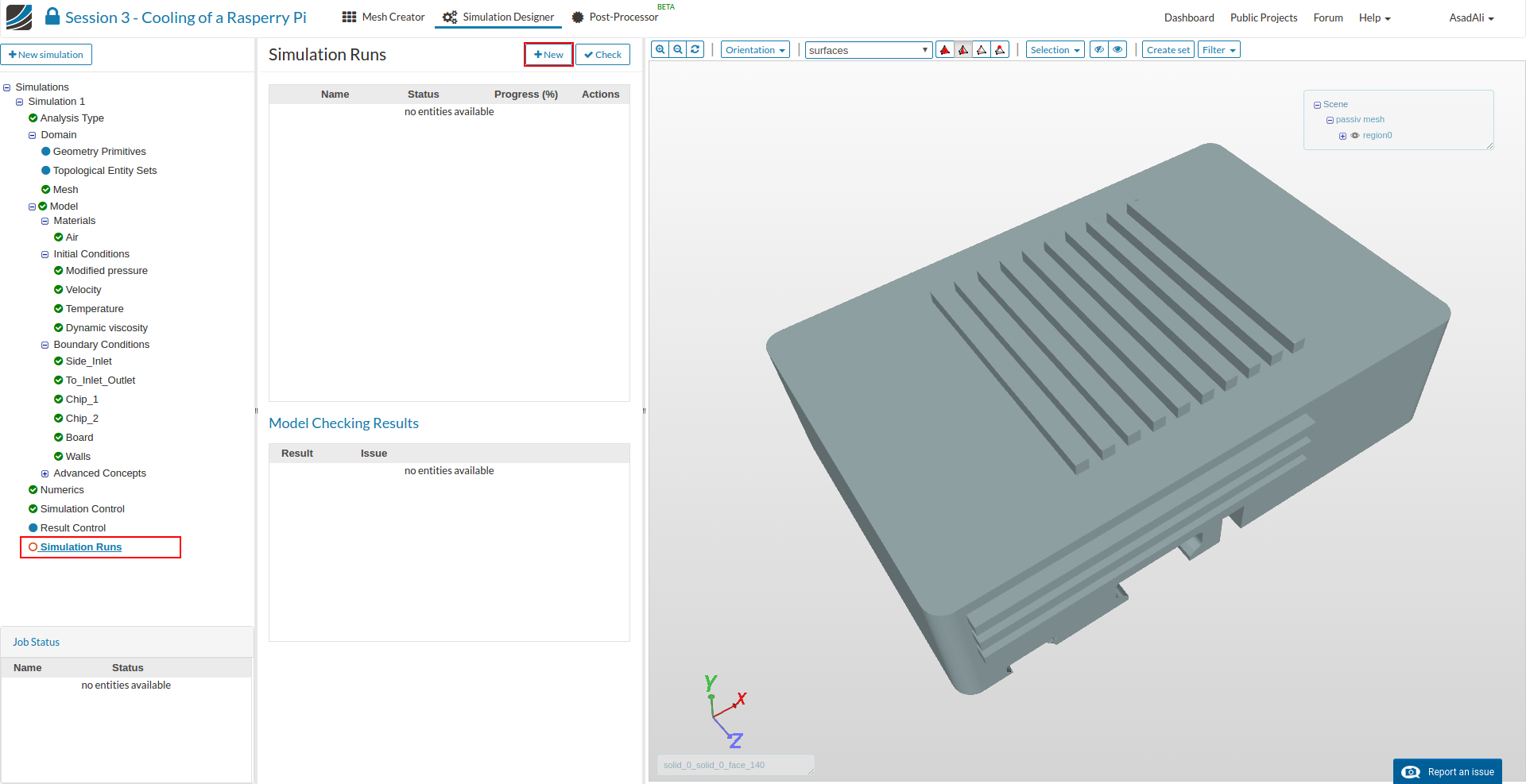
And start the simulation run by clicking the related button.
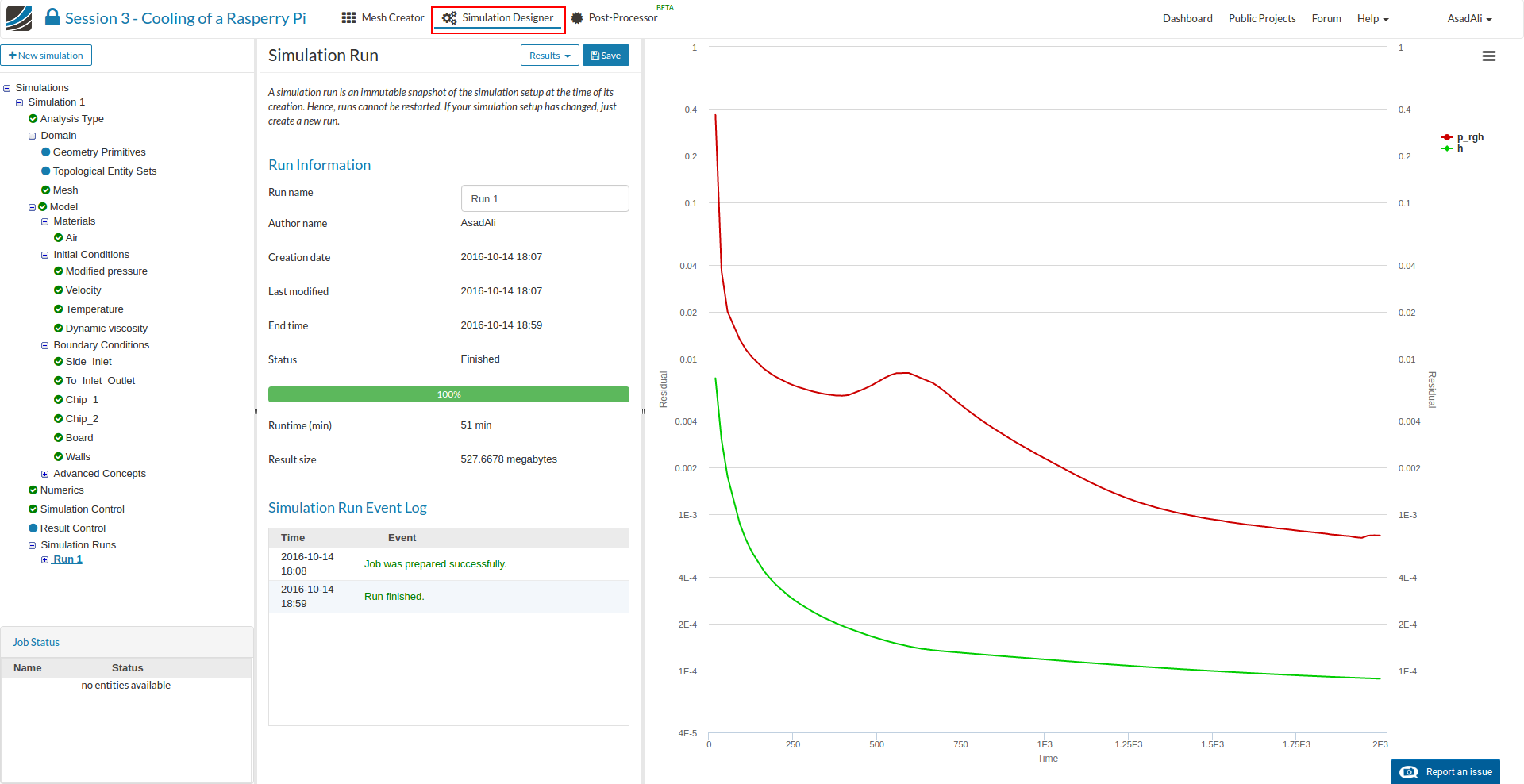
Post Processing
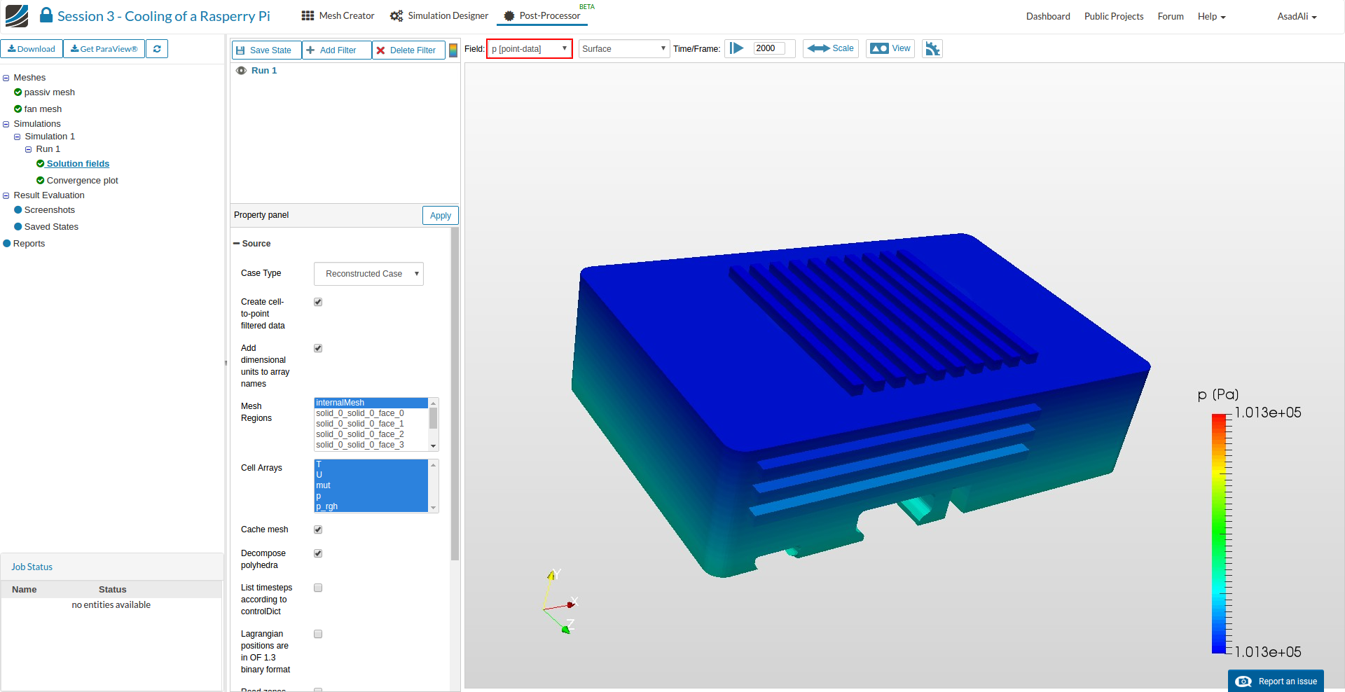
Once the simulation finishes, now to the Post-Processor tab And click on the Solution Field item in the project tree.
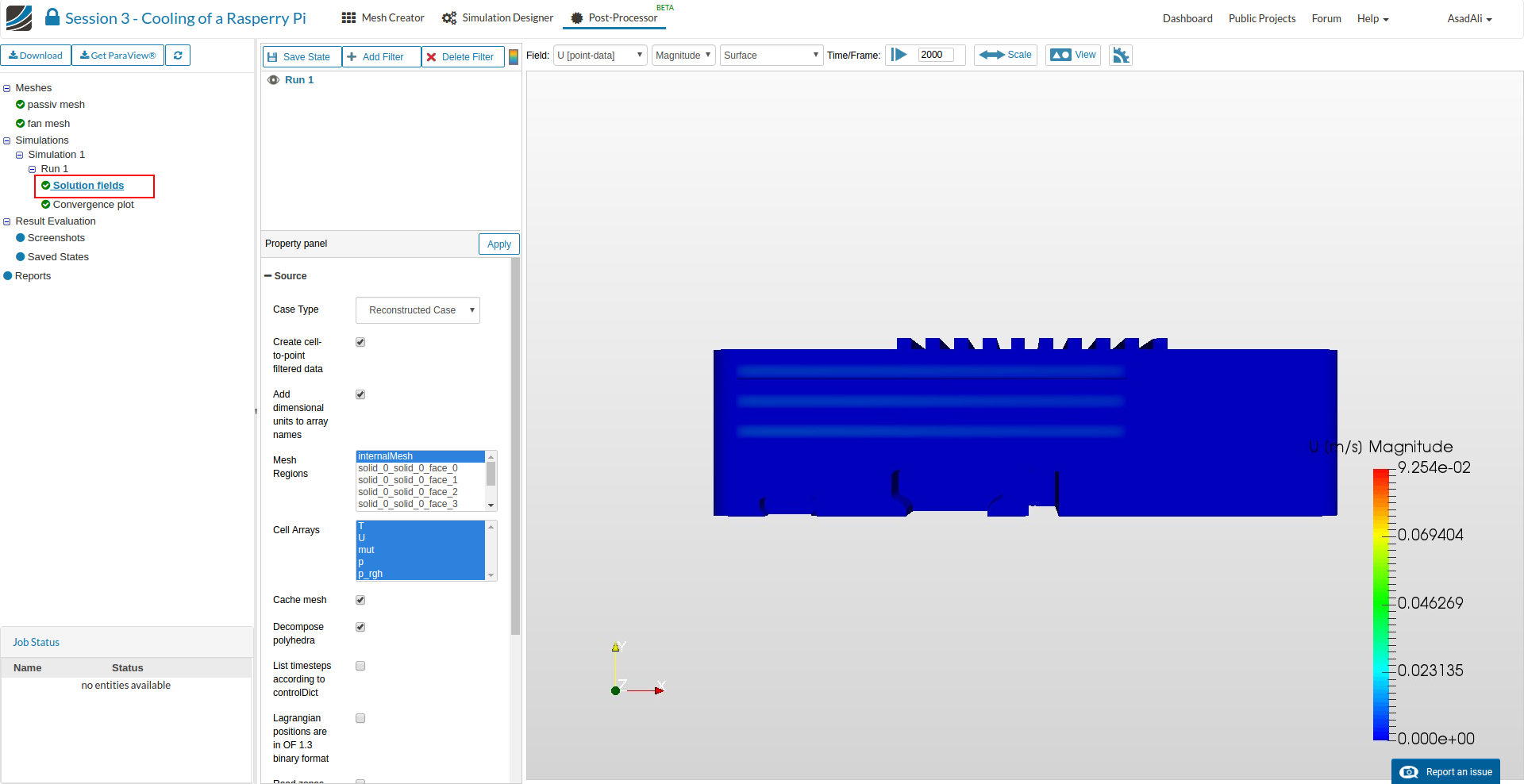
To visualize the pressure, change the plotted field to “p” by pressing the respective button.
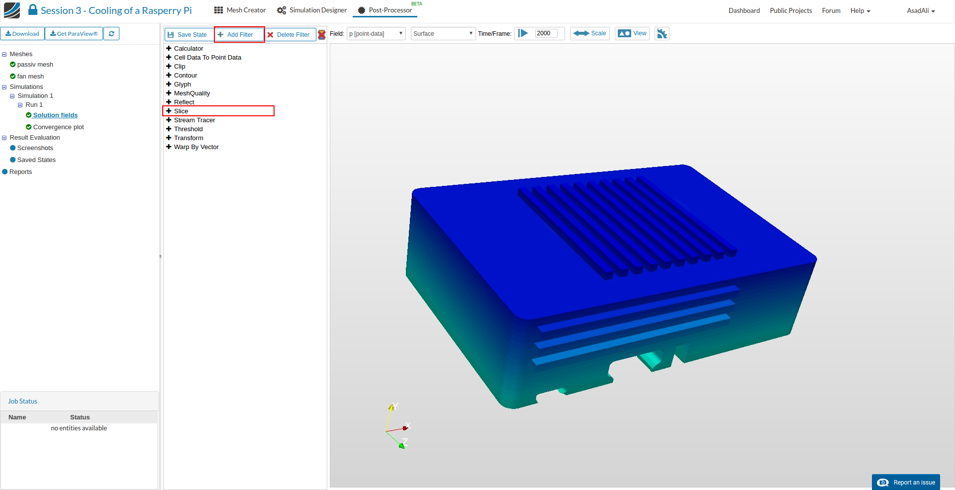
Now we can apply different filters on our simulation results to gain additional insights:
Slice-Filter
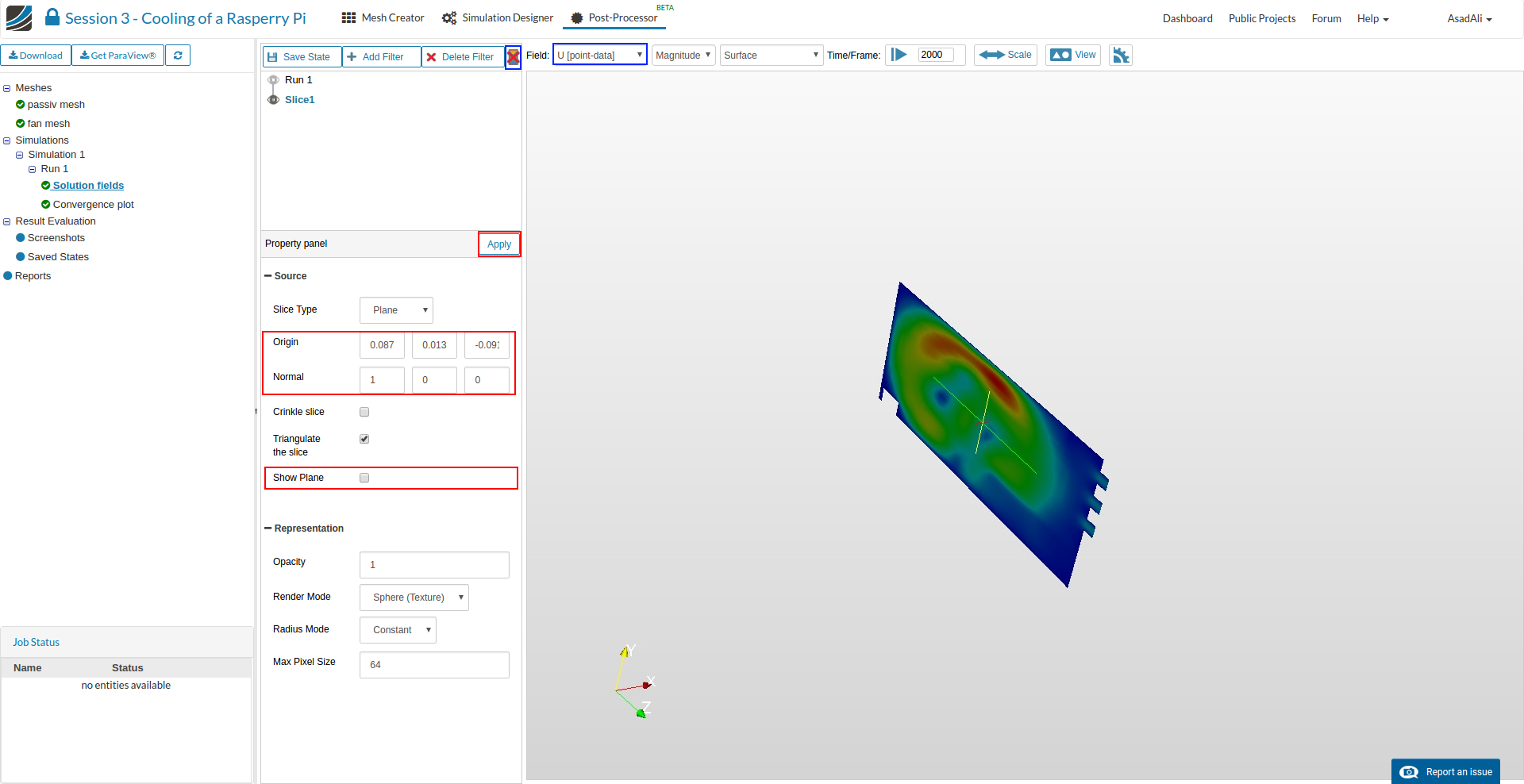
This filter isolates a slice through your mesh. It can help you to take a look inside the flow field. For this you only have to specify a plane by a point and a normal vector
You can manipulate the position of your slide my adapting the normal vector and the origin. Now let’s change the representation from pressure to velocity. Click on the left part of the drop down menu and change it to the field you want to show.
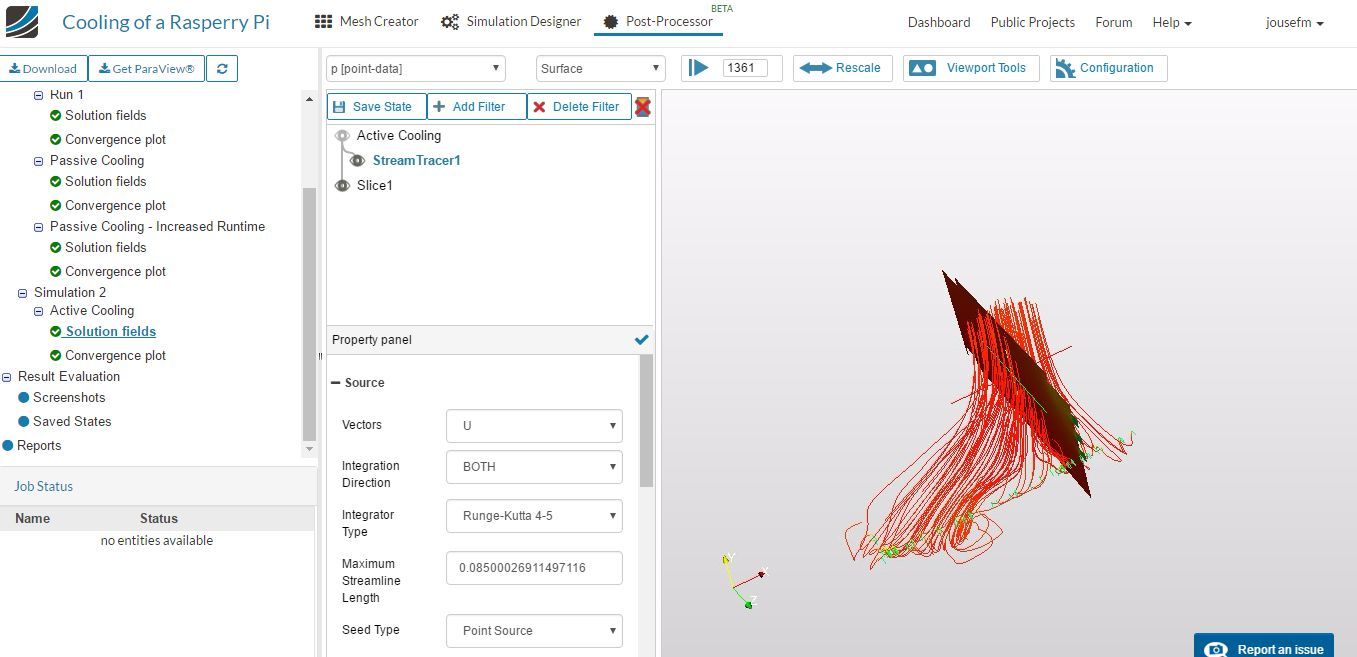
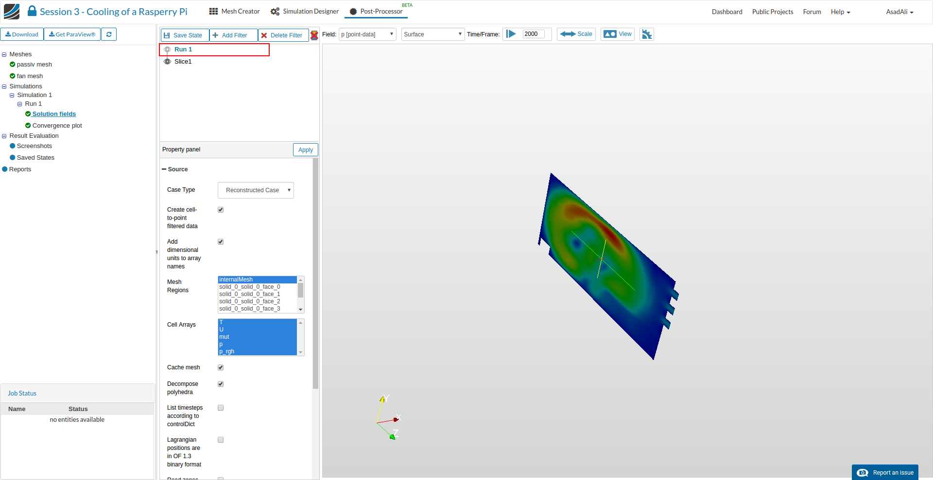
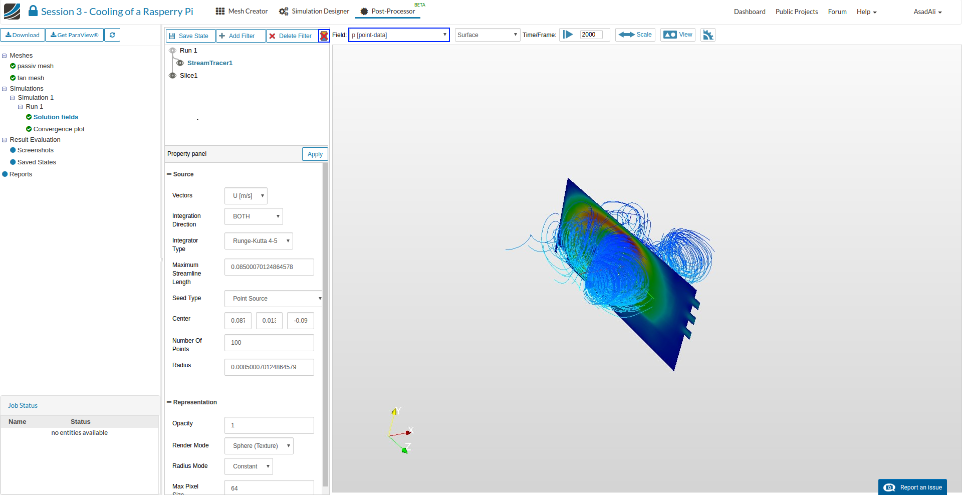
StreamTracer-Filter
We will now apply an addition filter to create stream lines which show us how the flow is streaming within the fluid domain. First of all you have to select the highest element of the post processing tree (Run 1) before you apply the next filter. Otherwise you would try to apply this filter on the slice.
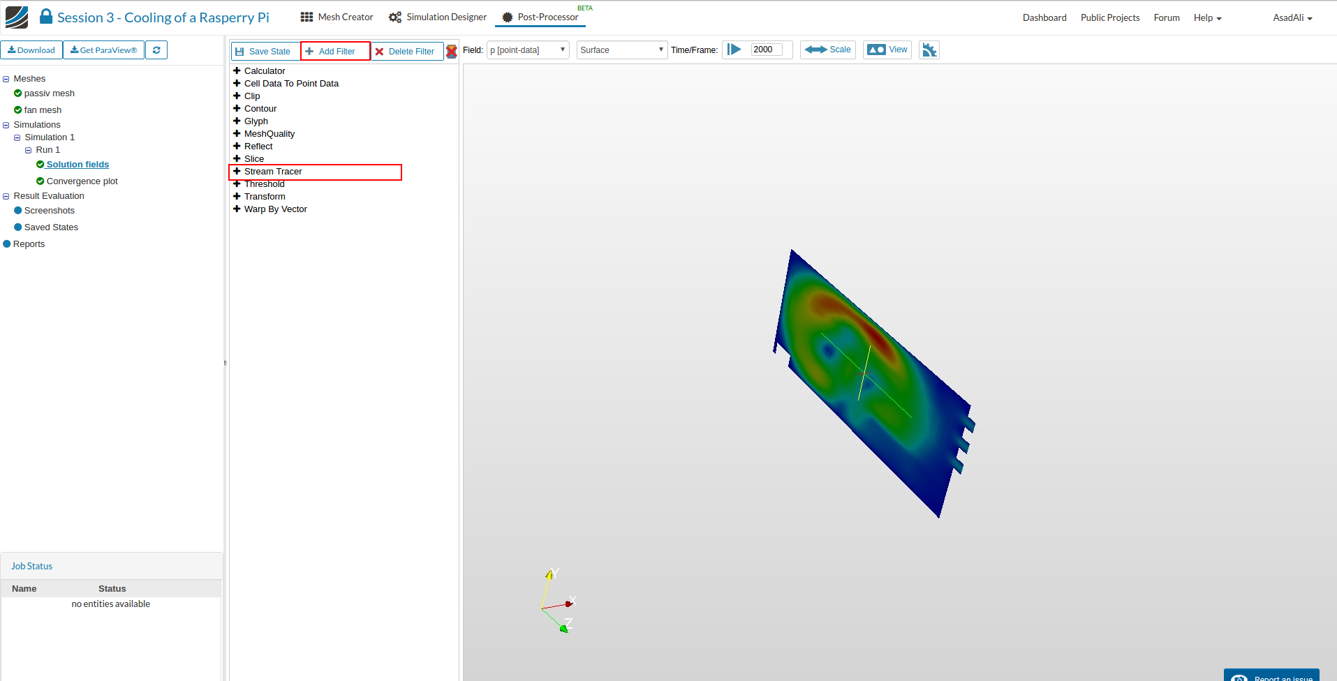
You can change the plotted fields, and show or hide the color legend.
Setup for Cooling
The steps for the simulation of the actively cooled housing are largely the same. However, there are small differences due to the different geometries, which are summarized here:
1. Meshing
The meshing operation (Hex-dominant automatic for internal flow (CFD)), and the parameters for Fineness and Parallel Processing be maintained.
2. Simulation Setup
For the initial conditions, only the values for the velocity must be adapted.
Since this setup is intended to simulate a fan and thus forced convection, it is necessary to change the boundary conditions for the inlet and the outlet.
We will use following boundary condition for the lateral louvers (outlet):
And following boundary condition for the fan inlet:
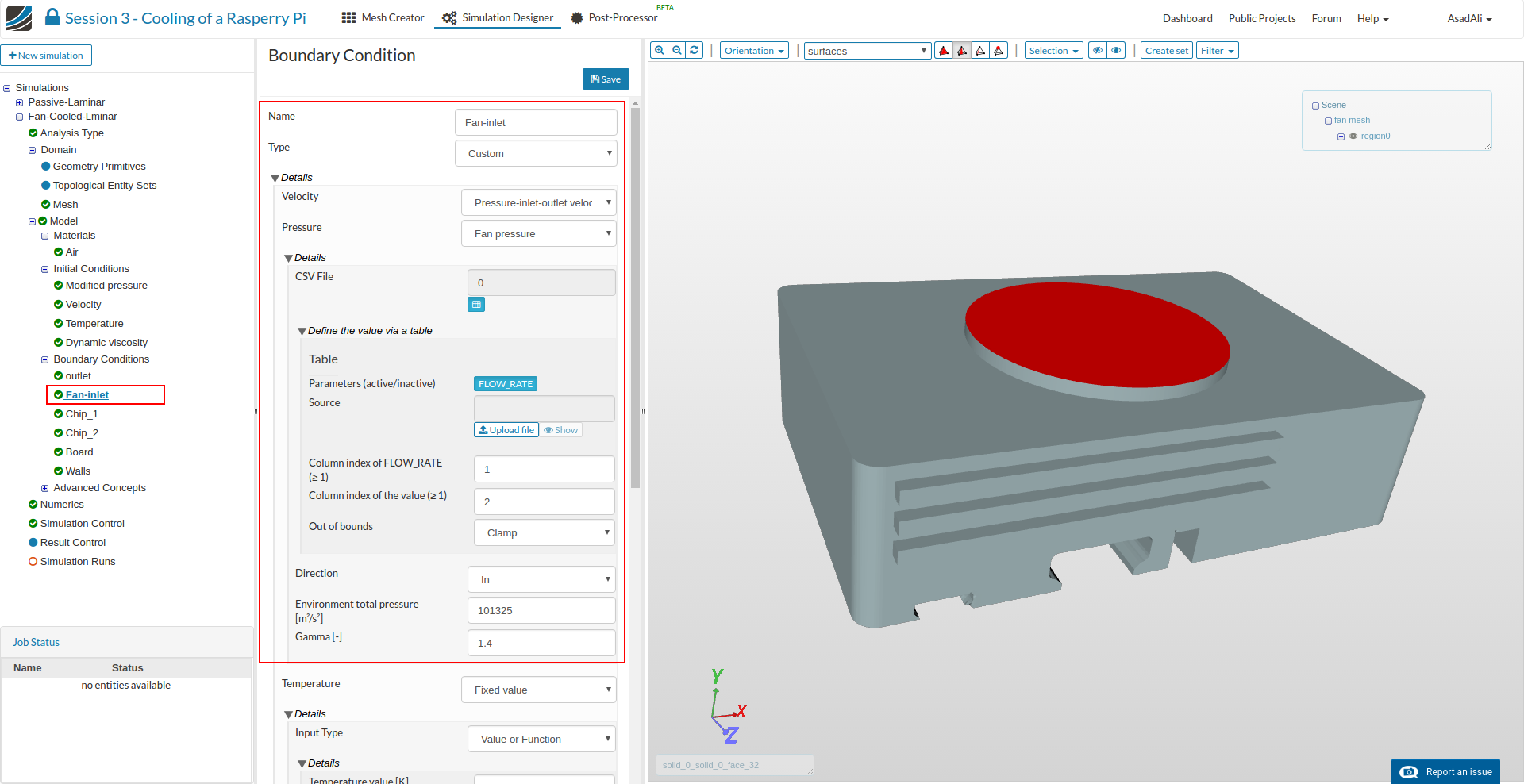
[The CSV file containing the fan curve]
(https://seafile.simscale.com/f/8cb2880188/?raw=1)
Other boundary condition, Chip_1, Chip_2, Board, Walls, are same as previous setup.
Finally, the numerical settings need to be adjusted: