Recording

Homework Submission
For your homework, your task is to setup a static structural analysis considering different material combinations for an artificial hip joint to better understand how stresses are transferred to the femur bone.
The step-by-step tutorial below contains all of the steps for setting up the simulation in SimScale and visualizing the results.
To submit your homework assignment, please generate a public link of your project (Sharing a Project)
Homework Deadline: Sunday, February 4th, 11:59 pm CET
Submit your homework here
Introduction
A hip joint prosthesis is used to replace a damaged hip joint. The most common materials used for artificial hip joints are metal alloys, ceramic or certain types of plastic. It is important to study these prostheses to understand how much compressive force will be transferred directly to the femur bone.
Ideally we would want a prosthetic joint component to carry stress in the same way as the original bone, however, this does not happen in real life.
According to the Department of Medicine at the University of Washington:
In a hip prosthesis, much of the load applied to the femoral component tends to be transmitted to the bone near its distal tip. The bone near the proximal part of the component tends to have less force transmitted through to it. What happens to the native bone that is now no longer receiving its usual loading? Bone loss occurs here. This phenomenon is called “stress shielding”. Since one can get quite a bit of stress shielding around a prosthesis, it’s no mystery why one sees progressive bone loss around prosthetic components over the years on follow-up radiographs.
The concept of stress shielding helps to explain the usual life course of a joint prosthesis. A hip prosthesis, for example, may last for 5 – 10 years before sufficient stress shielding occurs that the prosthesis loosens enough to be symptomatic. The loose prosthesis is then removed by the orthopedist, and a new one is put in. However, the native bone around the original femoral component now generally has substantially diminished bone stock. Therefore, the new one has to have a longer stem so that it will reach down far enough to seat in normal bone. This new prosthesis works for another 5 – 10 years, until stress shielding has caused enough bone resorption around this new prosthesis for it too to become symptomatically loosened. Then, a newer, even longer prosthesis is placed, and the cycle continues. Obviously, this process can’t go on forever, since you eventually run out of undisturbed bone in which to seat the prosthesis.
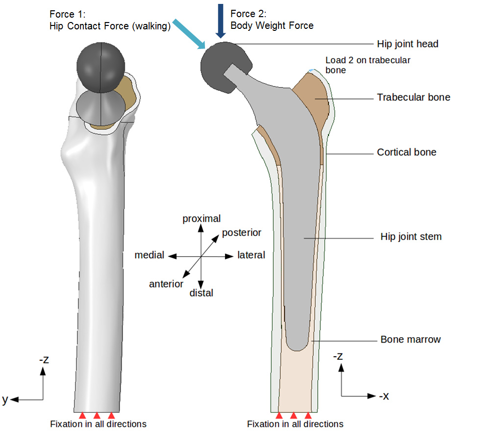
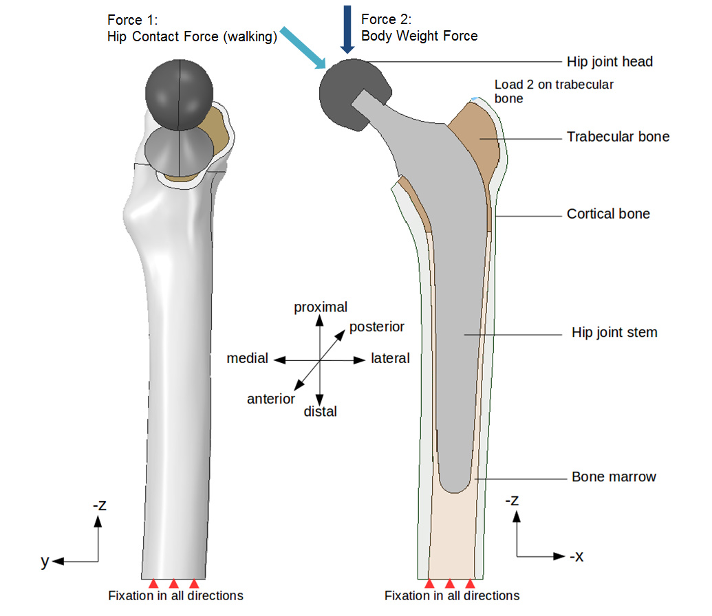
To set up the hip model for virtual simulation, the following loading conditions will be used:
-
The distal end of the bone is assumed to be fully fixed.
-
The body weight of the person is applied as a fixed force (Force 2).
-
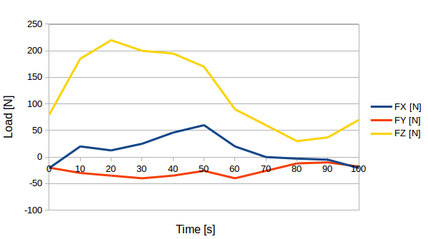
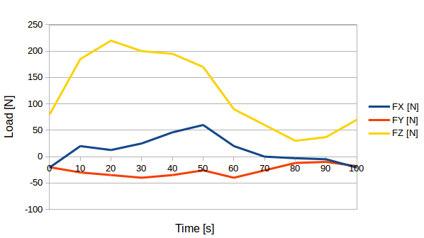
The hip joint head, which transfers the load from the upper body to the lower body is loaded with a variable force over 100 iterations (Force 1). See the graph below:
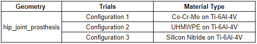
In this step-by-step tutorial, we will focus on a hip joint prosthesis model considering different material combinations for our artificial hip joint to better understand how stresses are transferred to the femur bone. You will perform 3 different simulations using the same geometry with different material combinations as shown:
Import Project
To start this exercise, please import the project into your workspace by clicking on the link below:
Mesh Generation
In the Mesh Creator tab, click on the geometry hip_joint_prosthesis
Then, click on the New Mesh button in the options panel.
Select the mesh Type Tet-dominant. This operation will automatically create a mesh for the geometry. The cell size and refinement will be adapted automatically. Please choose the following parameters:
- Element sizing: Automatic
- Mesh fineness: 3-Moderate
- Element order: First order
- Number of computing cores: 8
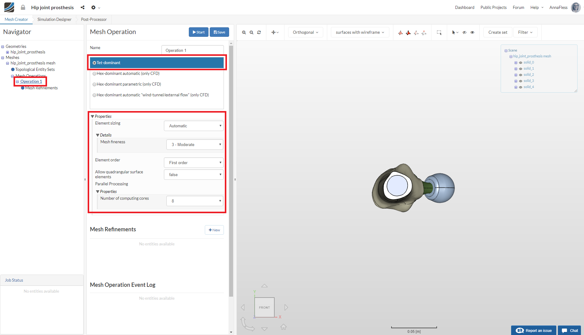
Click on Save to preserve the mesh settings
Now click the Start button to begin the mesh operation. The meshing job will start in a few moments (all of the computation is done via cloud computing).
The mesh operation takes about 5 minutes to complete. You will see the Finished status in the lower left corner when it is ready.
Simulation Setup
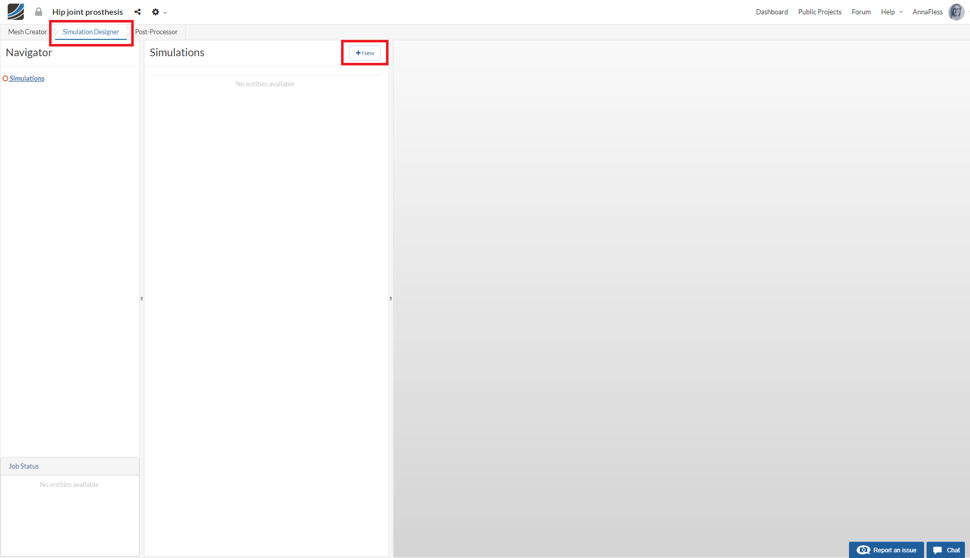
For setting up the simulation switch to the Simulation Designer tab and click +New to create a new simulation.
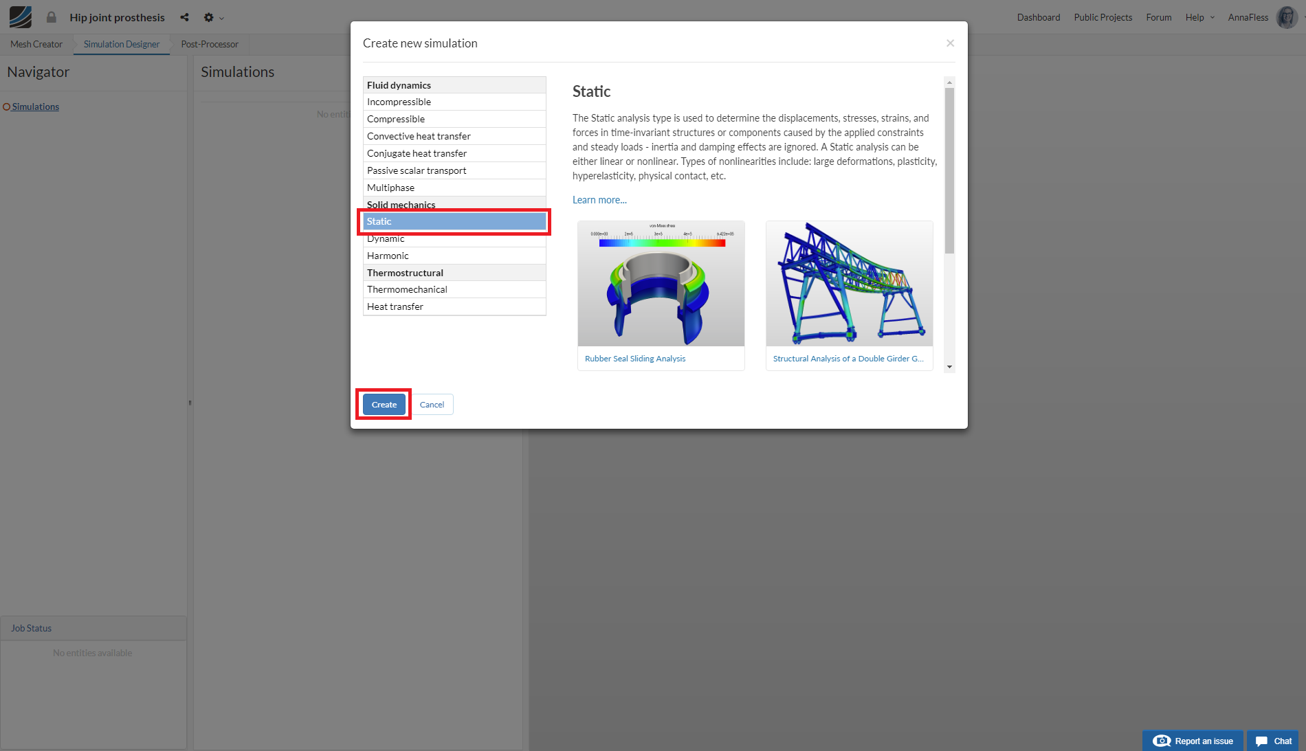
Since we want to evaluate the displacements, stresses, and strains on the hip prosthesis and femur, select the analysis type Static under Solid mechanics and then click create.
Give the project a name (optional) Co-Cr-Mo on Ti-6Al-4V and set the Nonlinear analysis option to true and click Save.
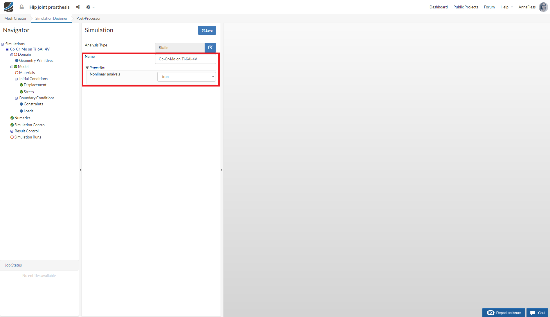
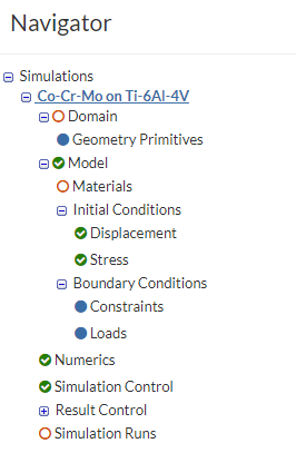
After saving, the Navigator now looks as shown below. Here the entries in red must be completed.
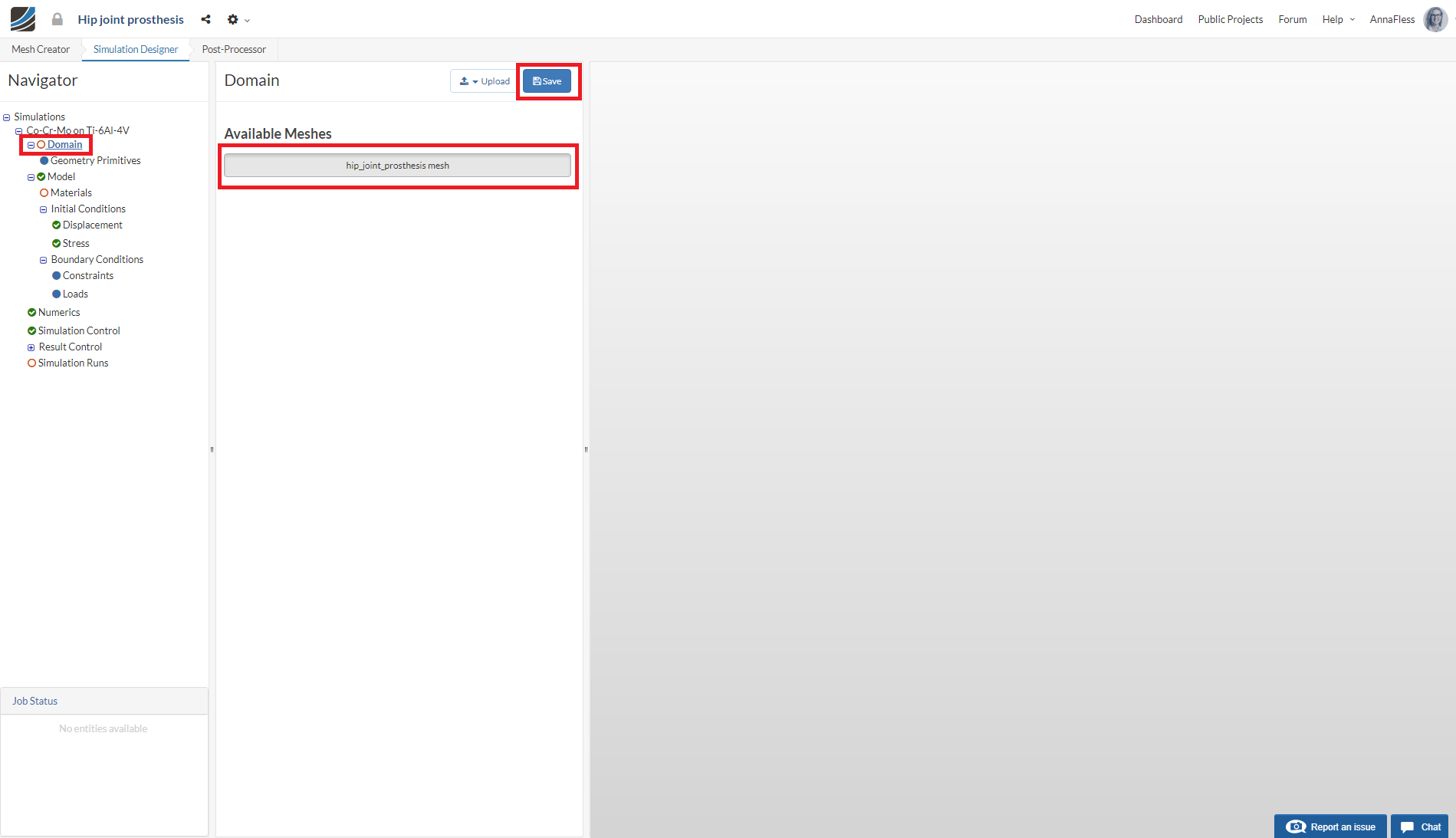
Click the Domain item in the Navigator and select the mesh that you just created. Click Save. The mesh will then automatically load in the viewer.
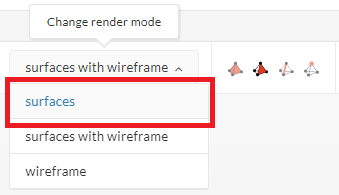
Next, change the render mode to Surfaces in the top viewer bar to interact with the mesh more easily.
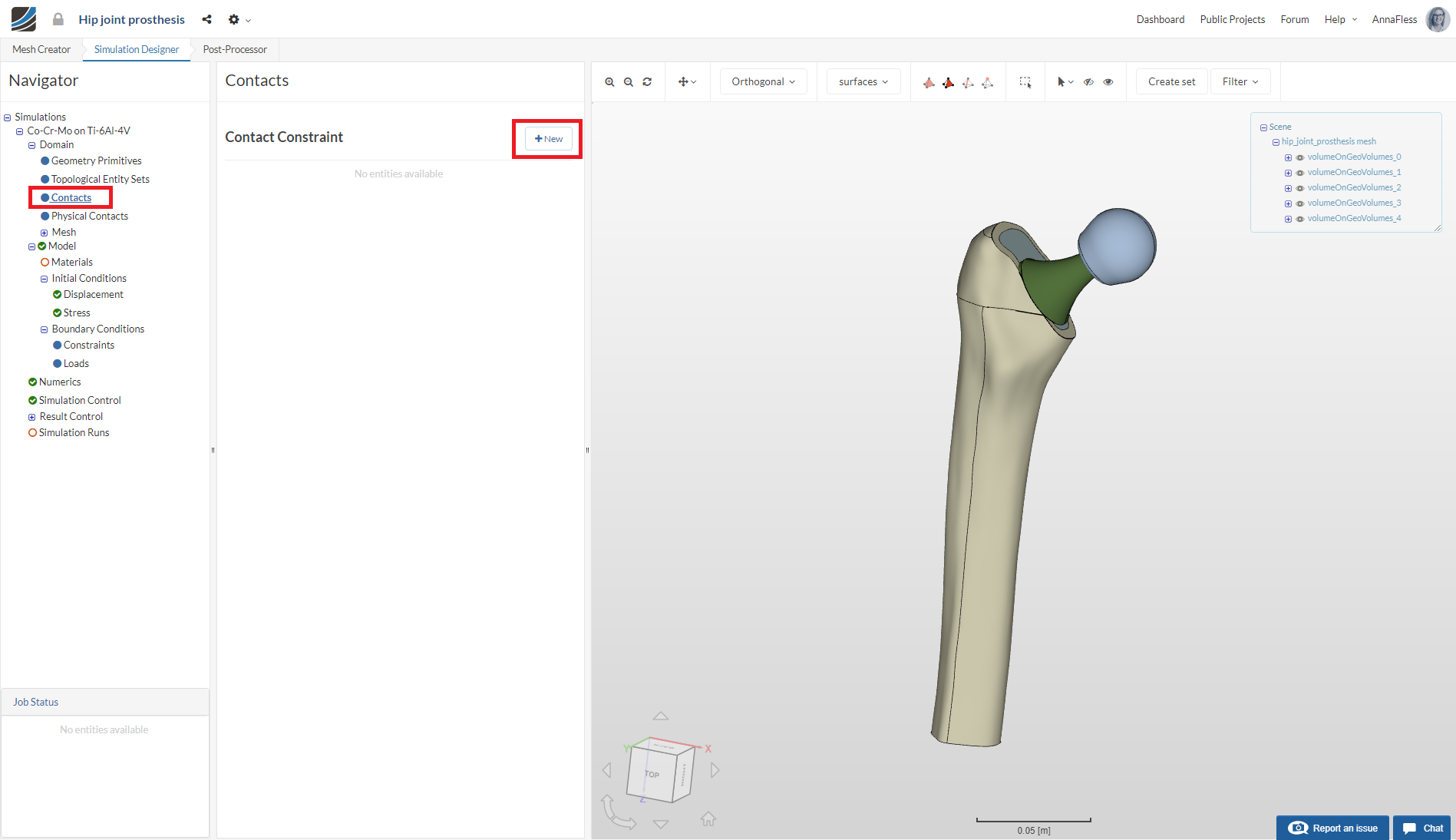
Contacts
Due to different material definitions for the bone and hip joint, we have to have a geometry that contains multiple volumes. These need to be bonded together so that the solver knows that they are connected. We will proceed with defining the bonded contacts between all of the solids.
Go to Contacts and click +New to create a new contact.
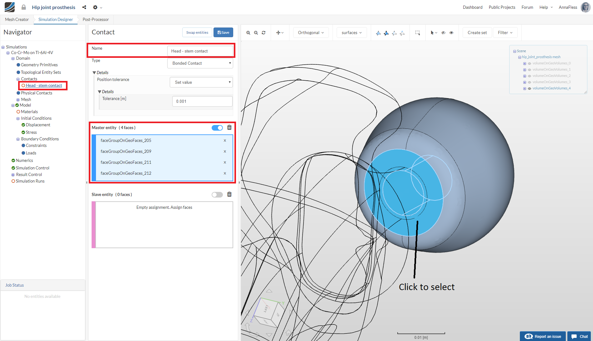
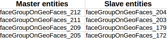
Head - stem contact
For creating a bonded contact between the head and stem of the hip joint, rename the contact definition to Head - stem contact (optional).
Hide all the volumes except volumeOnGeoVolumes_4 from the scene viewer in the top right.
Click to select all the faces of the head that will come in contact with the stem. Your selections will be automatically assigned to the Master entity (Blue).
Click on the Slave entity assignment box to activate selection.
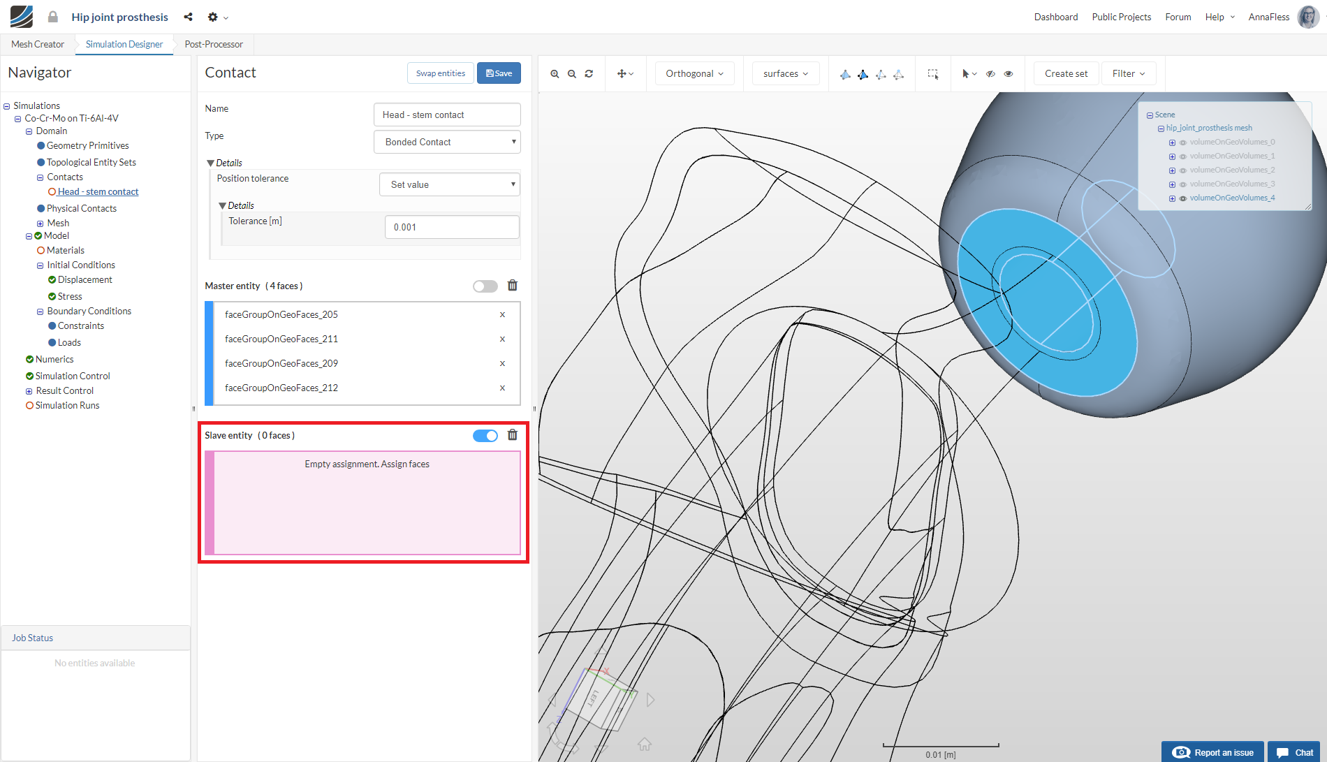
Then follow the same procedure for selecting the surfaces of the stem that are in contact with the head and assign these faces to the Slave entity.
Hide all the volumes except volumeOnGeoVolumes_3 from the scene viewer in the top right.
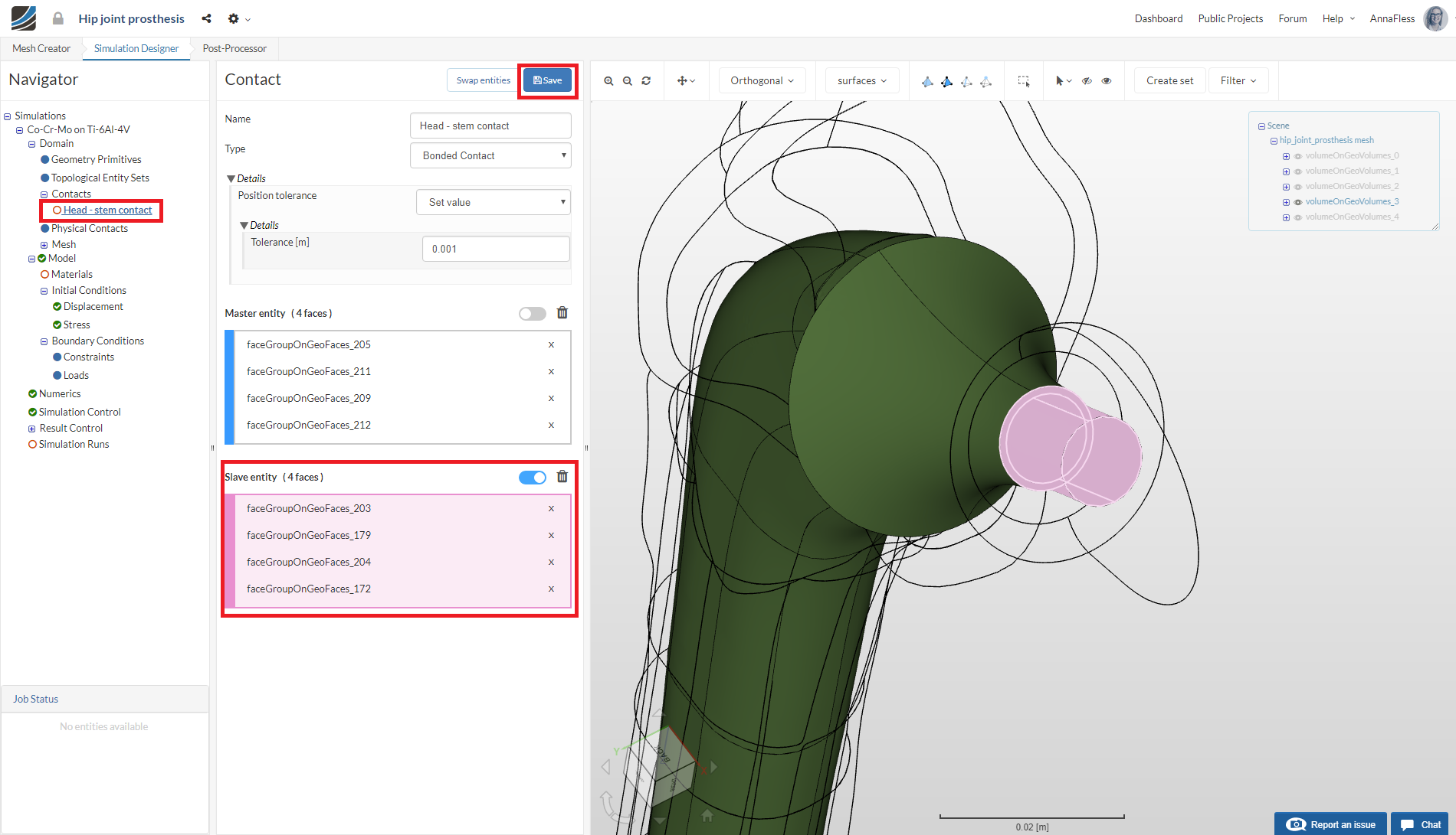
Click Save to create the contact.
To reconfirm, please make sure your selected entities match with those provided in the table below:
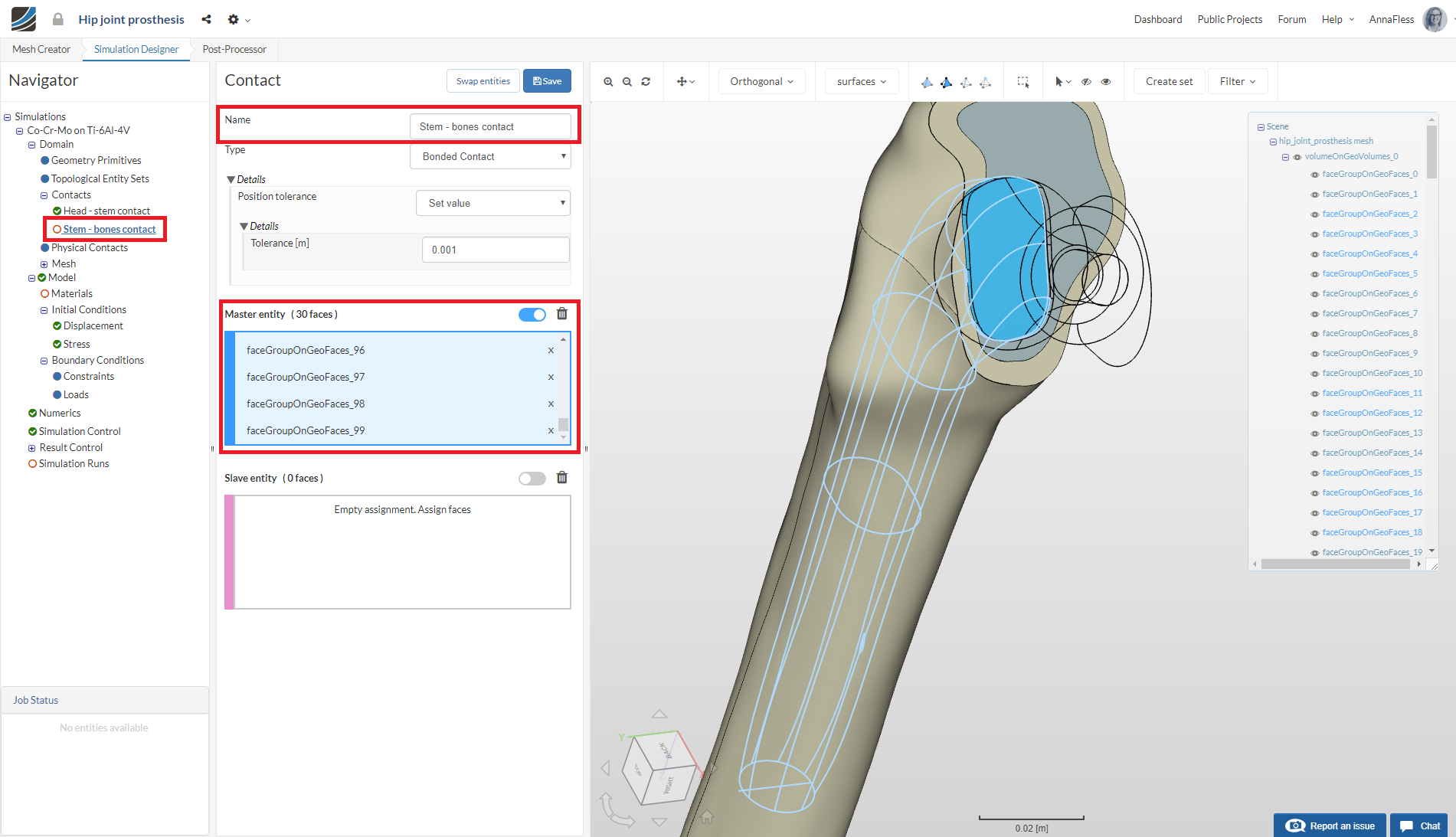
Stem - bones contact
Create a New Contact called Stem - bones contact and setup the contact between the stem and bones. Hide all of the solids except volumeOnGeoVolumes_0,volumeOnGeoVolumes_1 and volumeOnGeoVolumes_2
Select all of the internal surfaces that are in contact with the stem. Assign them as the Master entity.
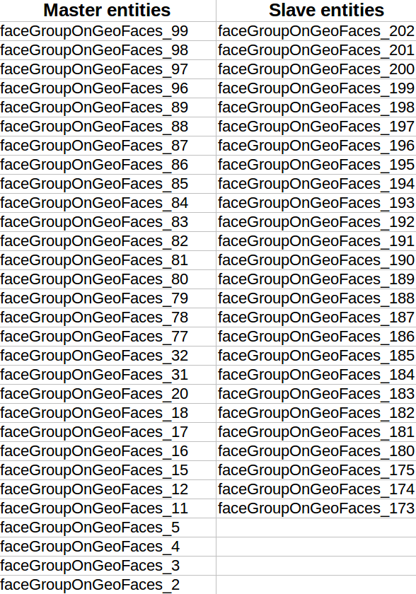
Click on the Slave entity assignment box to activate selection. Do the same for the stem and assign the faces as the Slave entity. Click Save to save the contact definition.
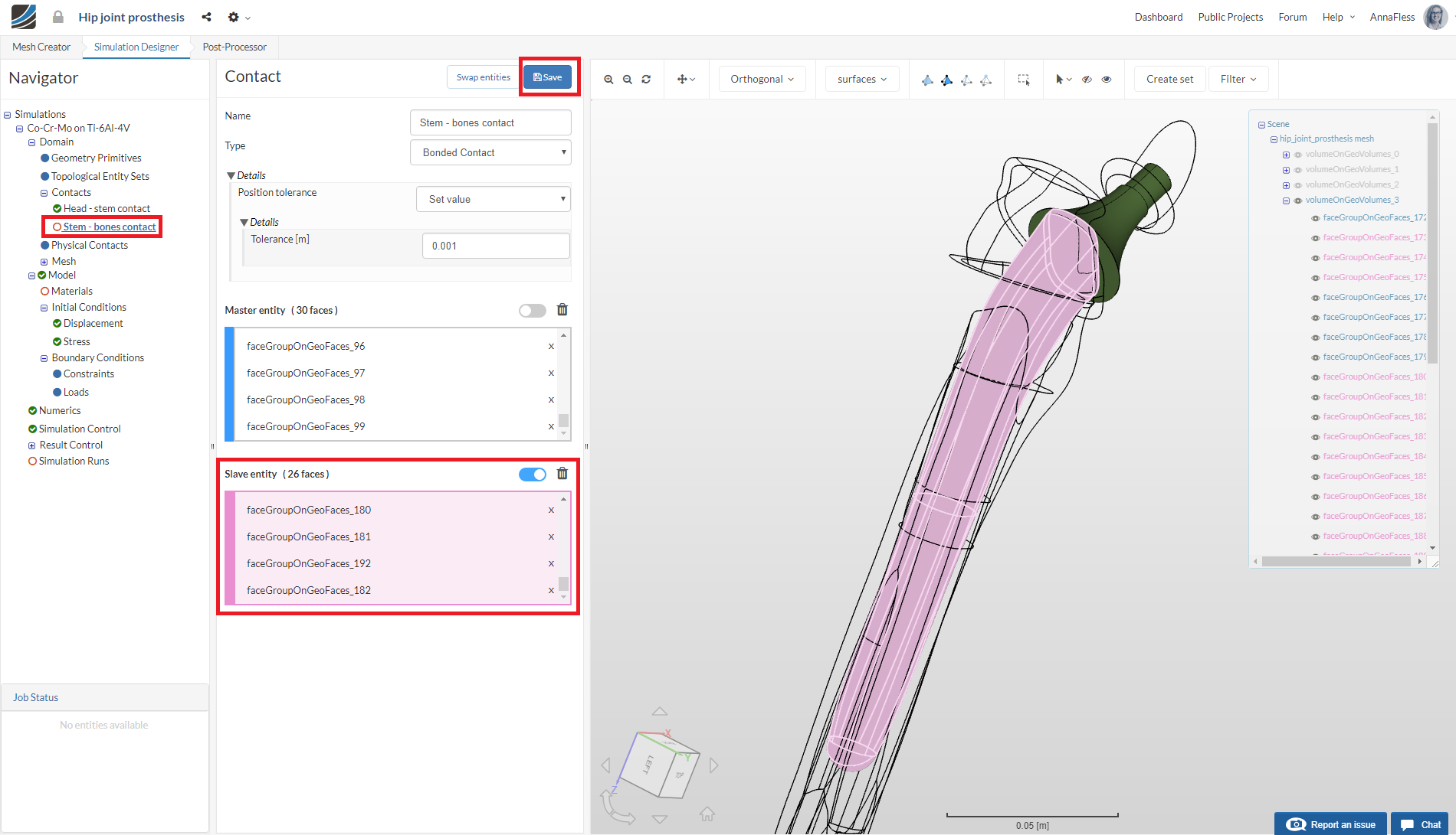
Hint: If you have problems selecting the faces in the Viewer, you can use the Scene viewer on the right of the screen to select faces. Double check that your selected entities match with those provided in the table below:
Trabecular - marrow contact:
Create a New Contact called Trabecular - marrow. Hide all volumes except volumeOnGeoVolumes_0. Select the lower face and assign it as the Master entity.
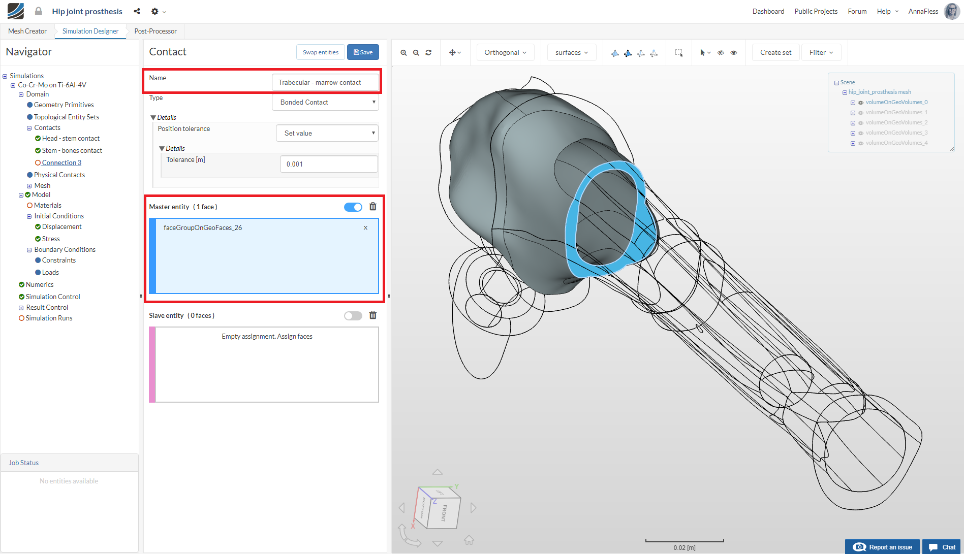
Click on the Slave entity assignment box to activate selection. Hide all volumes except volumeOnGeoVolumes_1. Select the lower face and assign it as the Slave entity. Click Save to save the contact definition.

To reconfirm, please make sure your selected entities match with those provided in the table below:
![]()
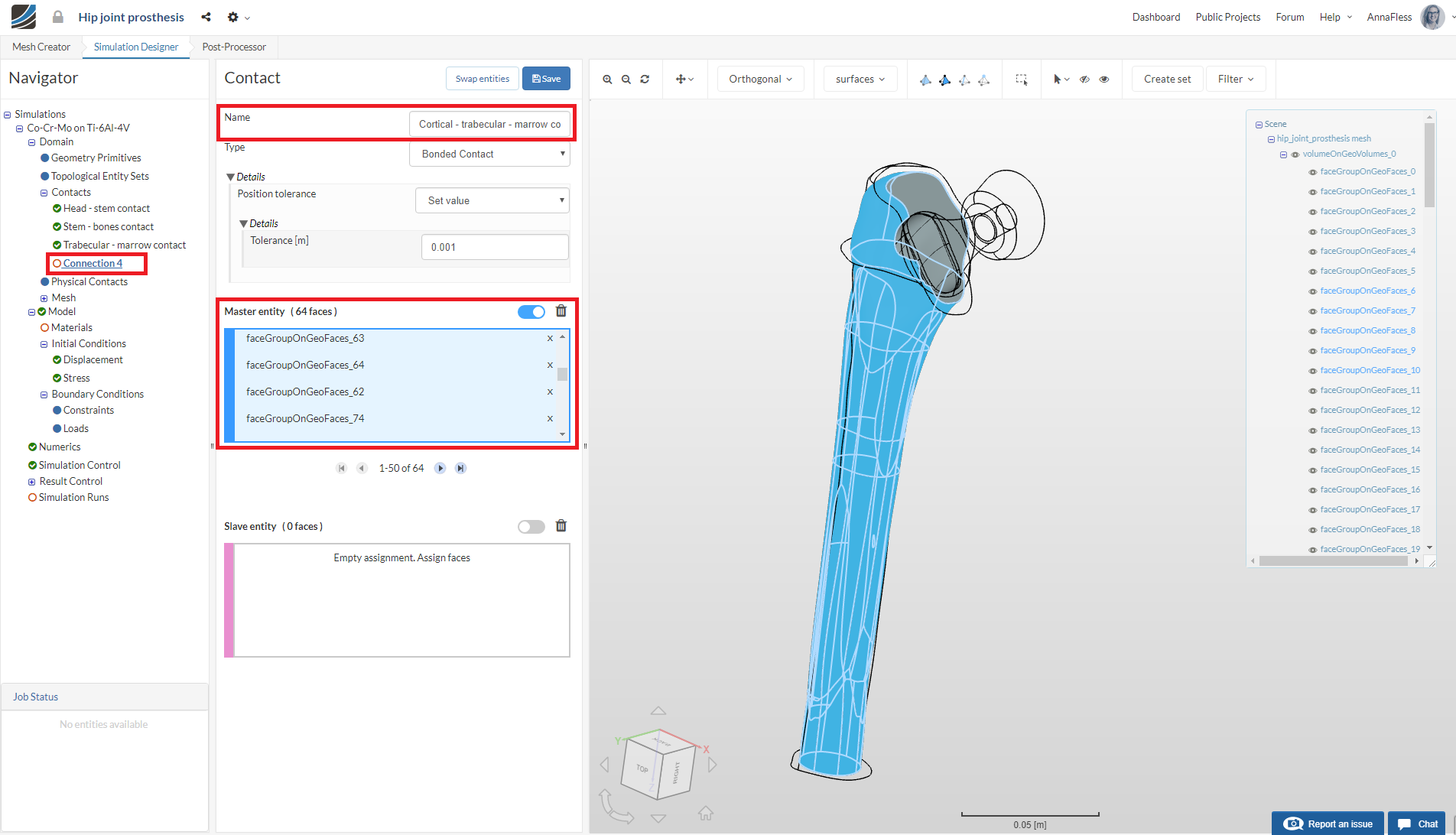
Cortical - trabecular - marrow contact
Create a New Contact called Cortical - trabecular - marrow contact. Hide all volumes except volumeOnGeoVolumes_0 and volumeOnGeoVolumes_1. Select all of the outer faces and assign them as the Master entity.
Click on the Slave entity assignment box to activate selection. Now hide all volumes except volumeOnGeoVolumes_2. Select all of the internal faces and assign them as the Slave entity. Click Save to save the contact definition.
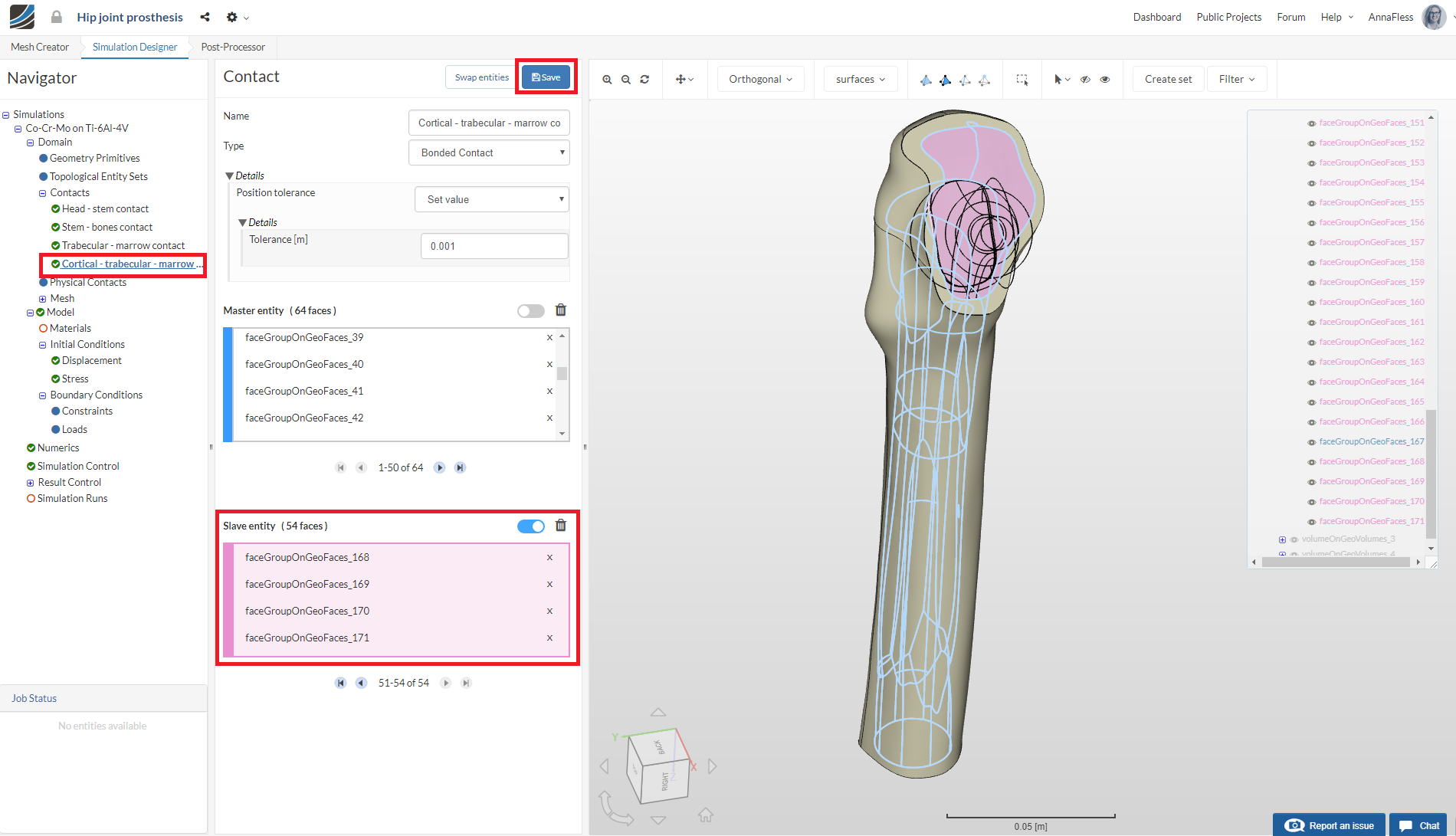
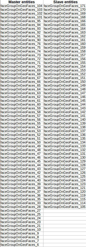
To reconfirm, please make sure your selected entities match with those provided in the table below:
Now that the contacts are set up, we will define the material definition for all of our volumes. The material definition for the bones and the hip joint are taken from reference [1].
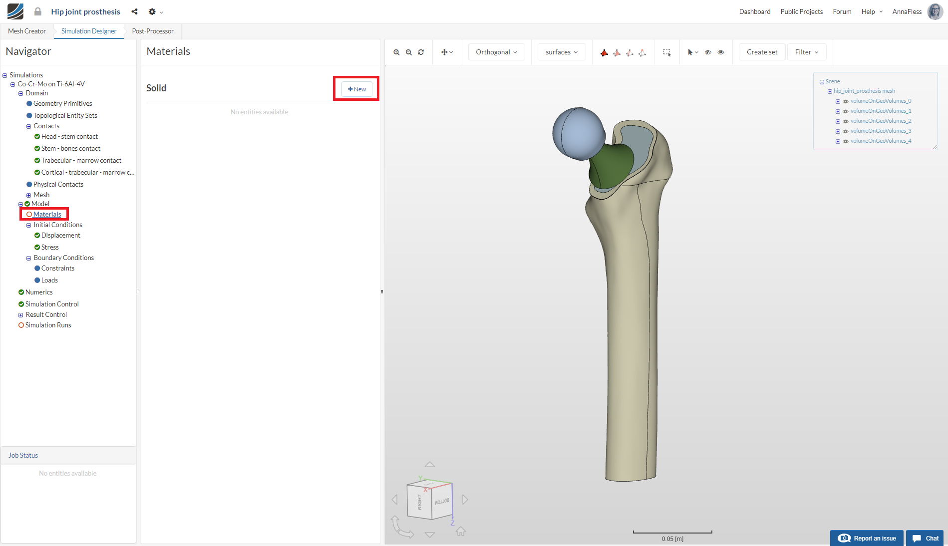
Materials
Go to the Materials item in the Navigator and click + New
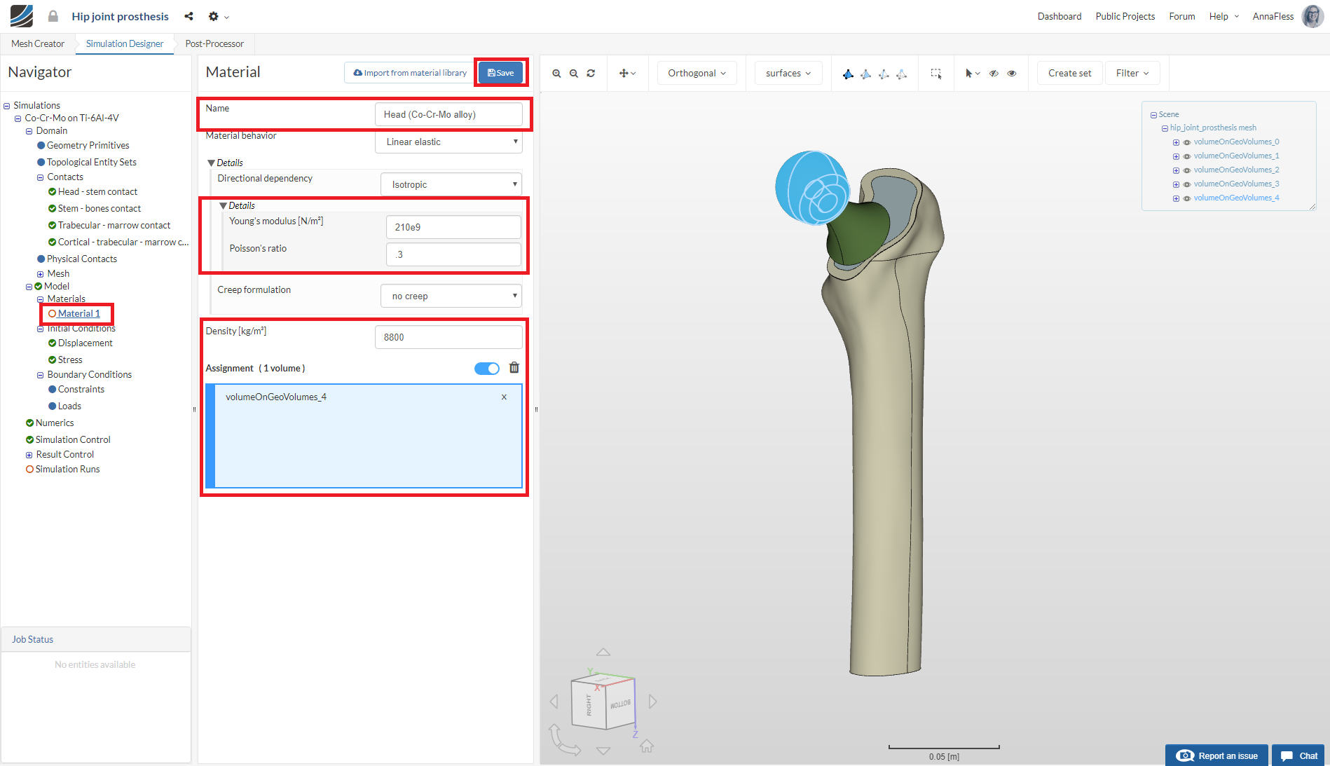
Head (Co-Cr-Mo alloy)
First we will define the material for the hip joint head. Rename the newly created material to Head (Co-Cr-Mo alloy) (optional).
Change the Young’s modulus, Poisson’s ratio and Density values to 210e9, 0.3, and 8800 as shown in the figure below.
Assign the material to volumeOnGeoVolumes_4.
Click Save to save this material definition.
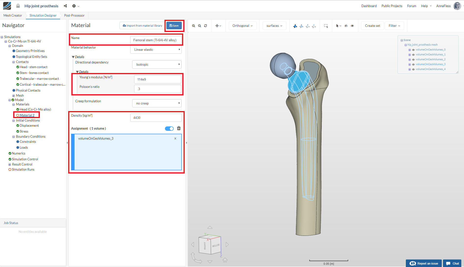
Femoral stem (Ti-6Al-4V alloy)
Proceed with the same steps as above to create a new material. Rename the newly created material to Femoral stem (Ti-6Al-4V alloy) (optional).
Change the Young’s modulus, Poisson’s ratio and Density values to 114e9, 0.3, and 4430 as shown in the figure below.
Assign the material to volumeOnGeoVolumes_3.
Click Save to save this material definition.
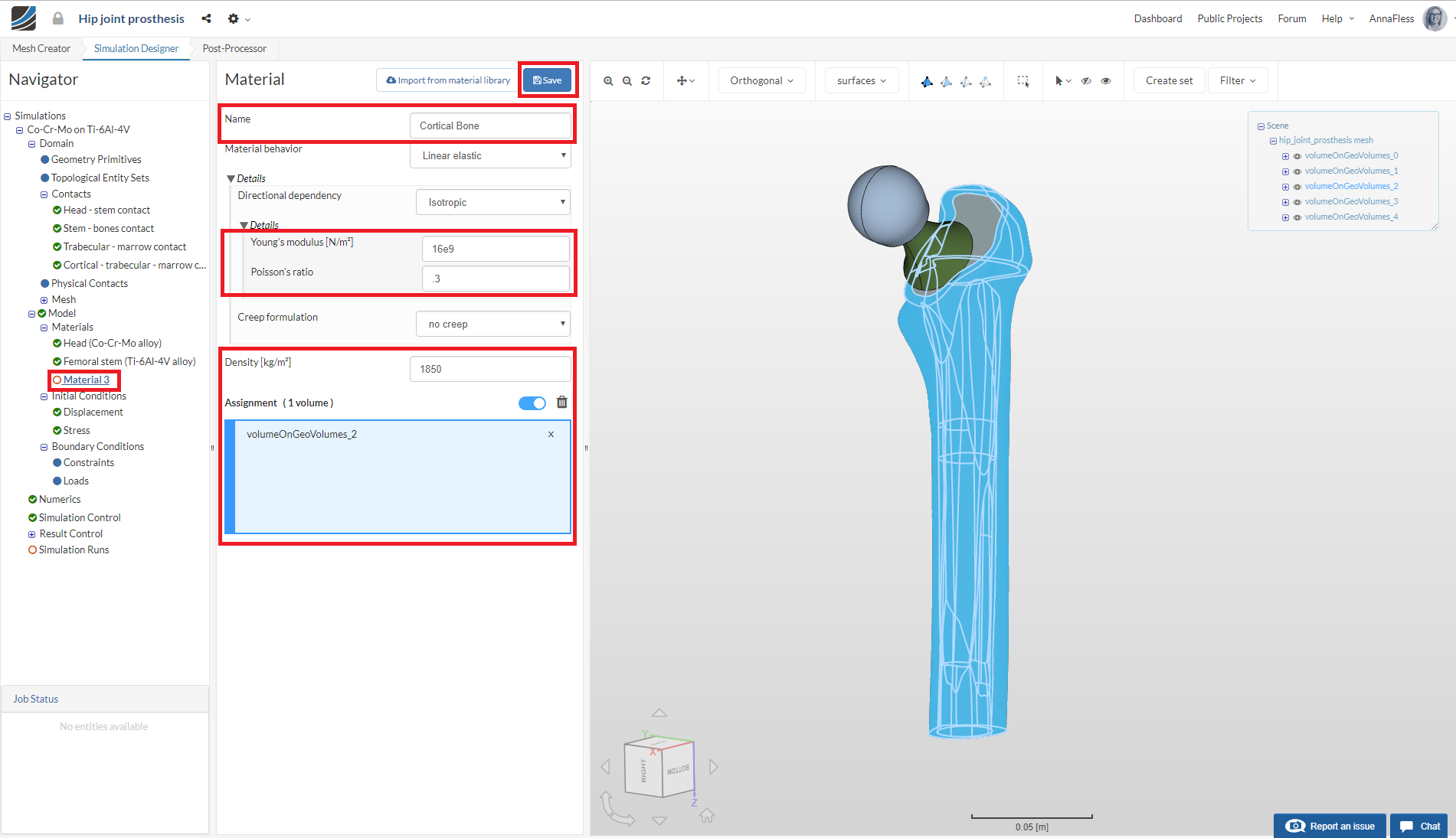
Cortical bone
Proceed with the same steps above to create a new material. Rename the newly created material to Cortical bone (optional).
Change the Young’s modulus, Poisson’s ratio and Density values to 16e9, 0.3, and 1850 as shown in the figure below.
Assign the material to volumeOnGeoVolumes_2.
Click Save to save this material definition.
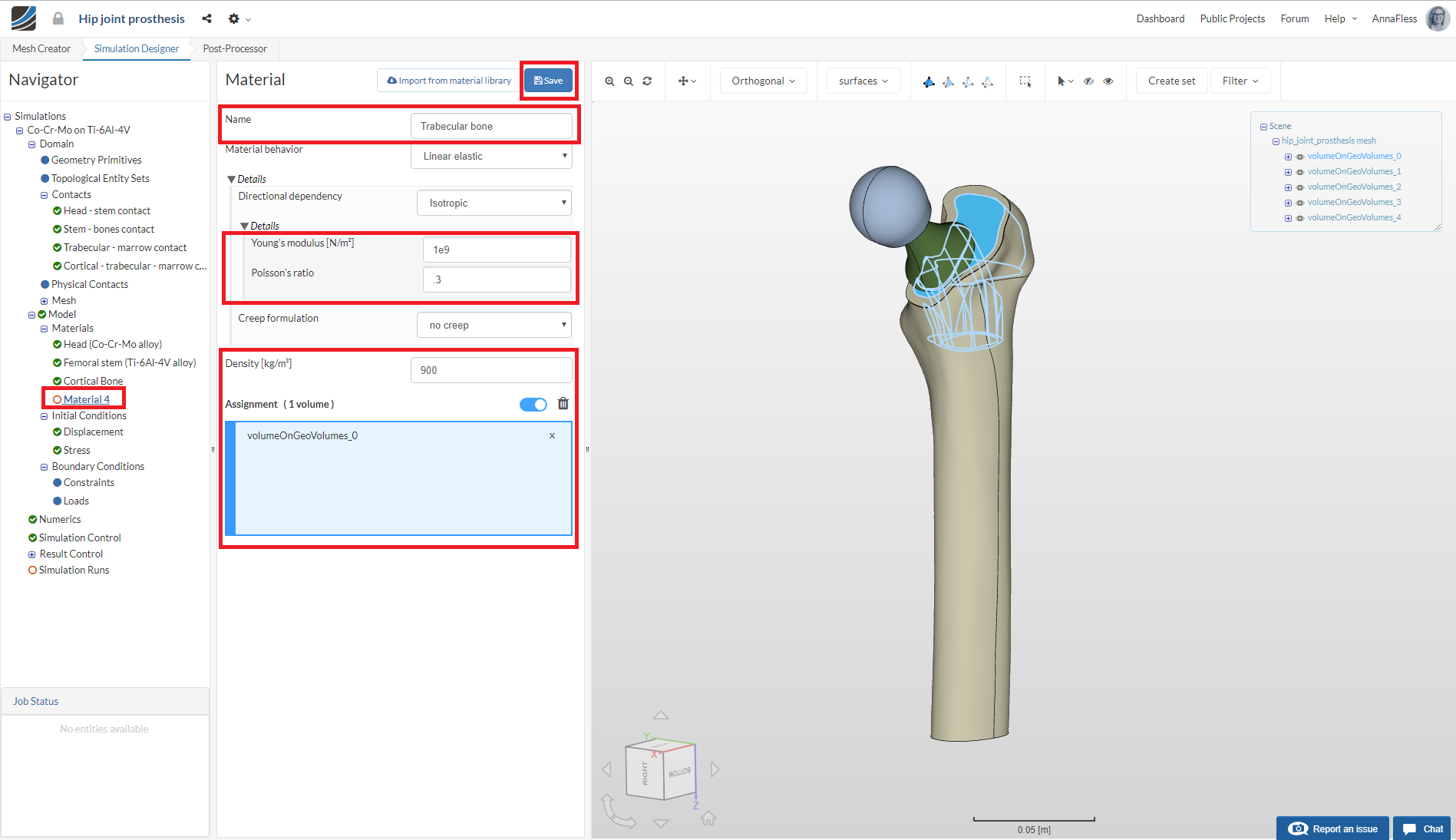
Trabecular bone
Proceed with the same steps above to create a new material. Rename the newly created material to Trabecular bone (optional).
Change the Young’s modulus, Poisson’s ratio and Density values to 1e9, 0.3, and 900 as shown in the figure below.
Assign the material to volumeOnGeoVolumes_0.
Click Save to save this material definition.
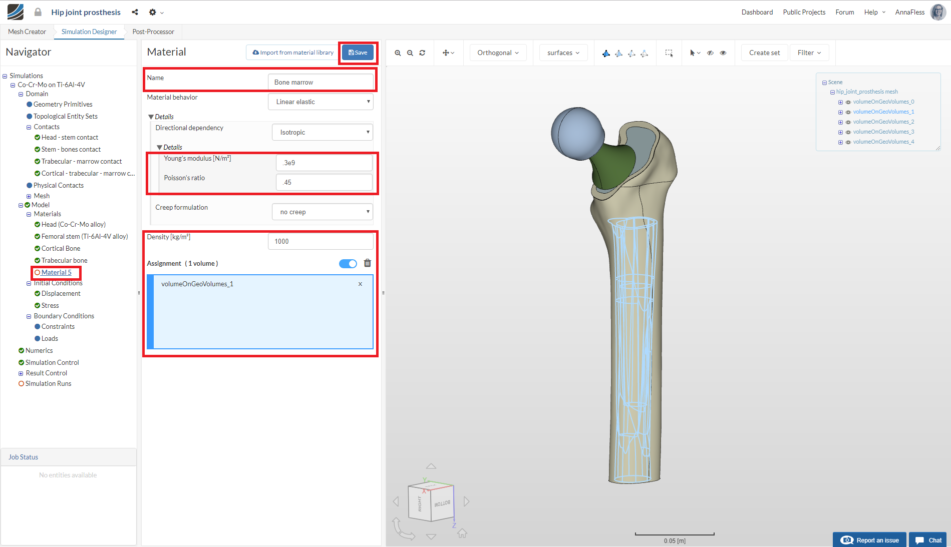
Bone marrow
Proceed with the same steps above to create a new material. Rename the newly created material to Bone marrow (optional).
Change the Young’s modulus, Poisson’s ratio and Density values to 0.3e9, 0.45 and 1000 as shown in figure below.
Assign the material to volumeOnGeoVolumes_1.
Click Save to save this material definition.
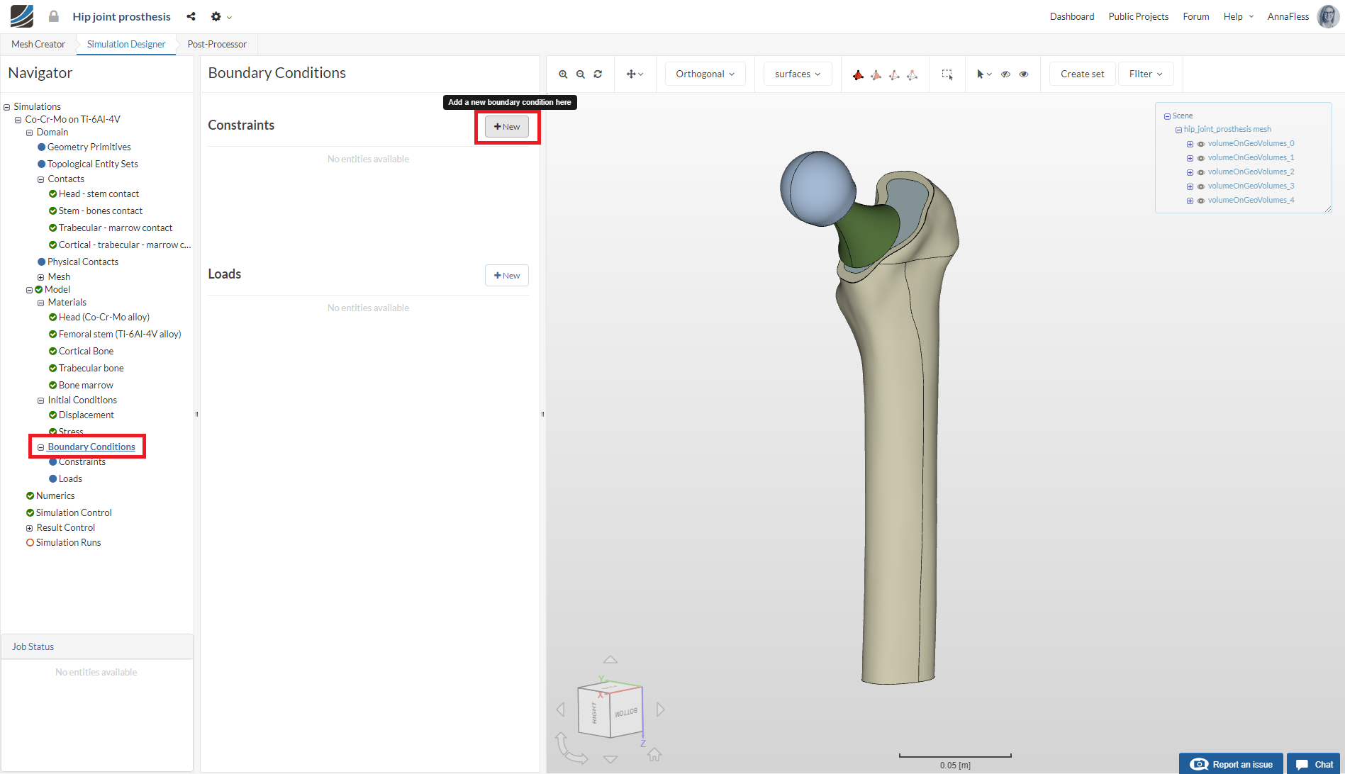
Boundary Conditions
We will now proceed the constraint and load definitions for our simulation case, as shown in figure below.
Go to the Boundary Conditions item in the Navigator and click +New next to Constraint to first define the fixation boundary condition.
Fixation
Rename the newly created constraint to Fixation (optional). Select Fixed support as the Type.
Make sure the Filter for entity types to faces under Topological Mapping
Select the bottom two faces of the model.
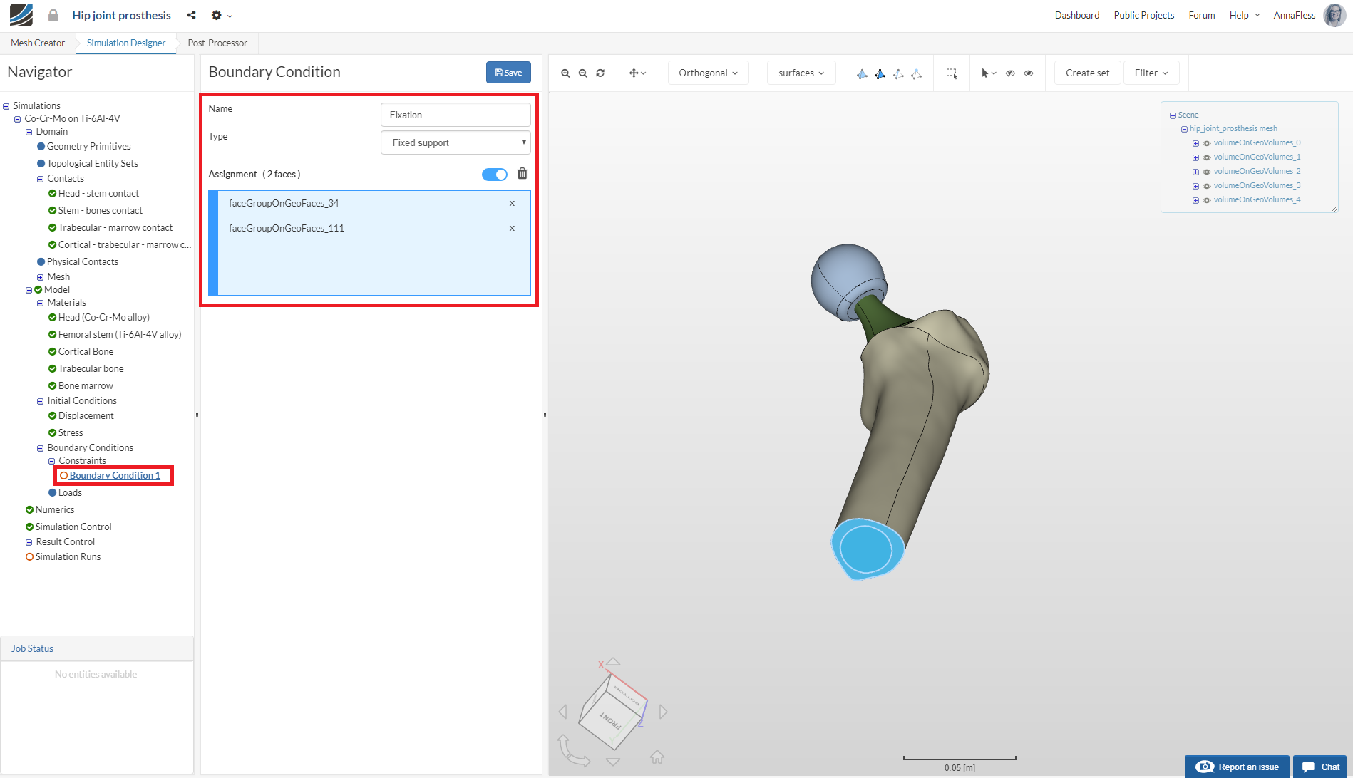
Click Save to save the constraint definition.
Load 1
Next we will define our first load boundary condition on the femur hip joint head for the hip contact forces when a person is walking.
This will be applied as a variable load, as shown below:
Proceed to Loads under tree and click +New to create a new load definition.
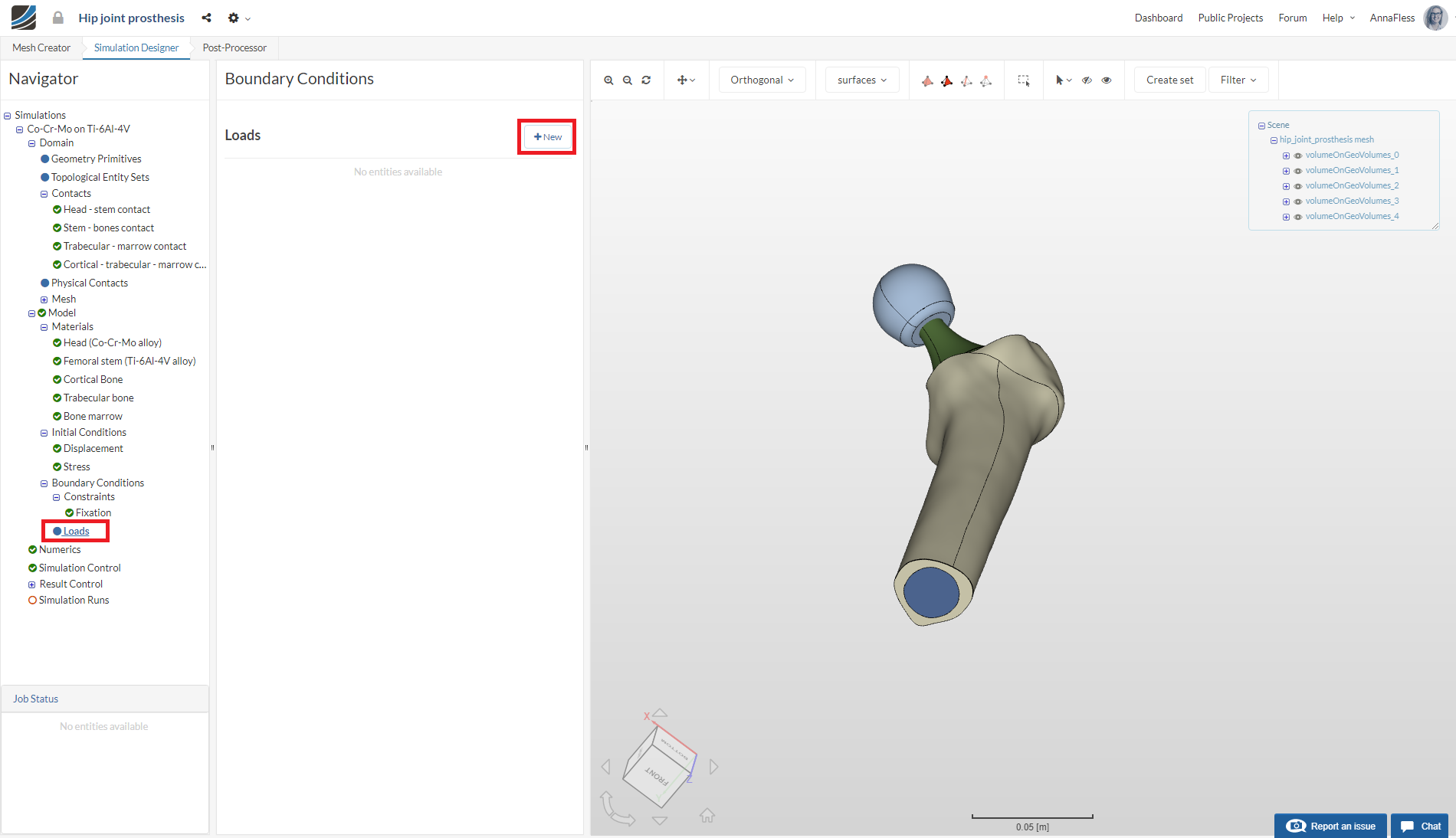
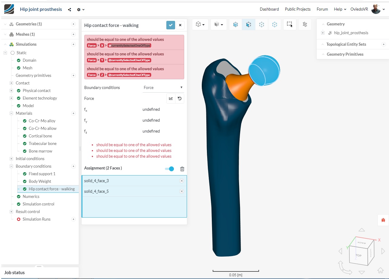
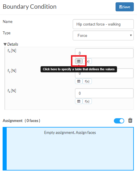
Rename the newly created constraint to Hip contact force - walking (optional). Select Force as the Type.
To apply the load in this case, we need upload a table that specifies the values over time.
Download the .csv file here: https://drive.google.com/file/d/1iAlXsylhDkfs_N4TBsdafTXIEtkBjAdw/view?usp=sharing
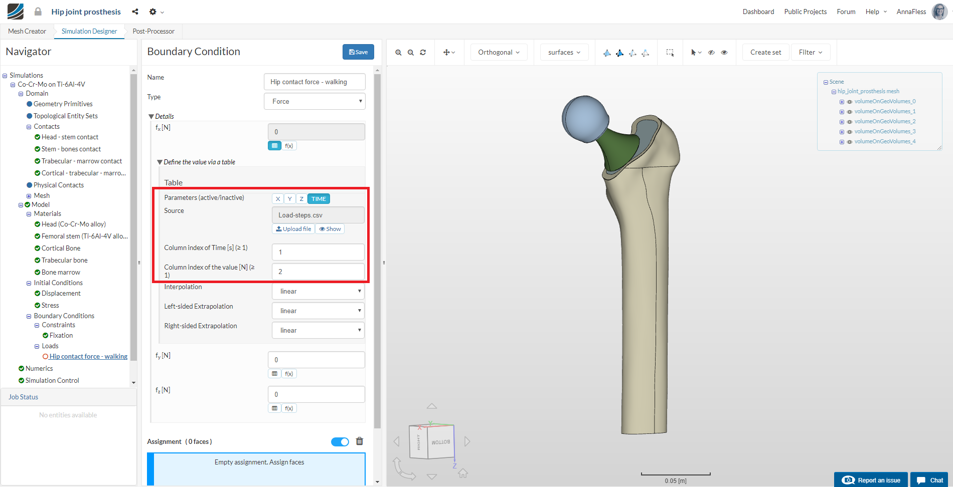
Click on the table upload icon for fx
Then click on Upload file
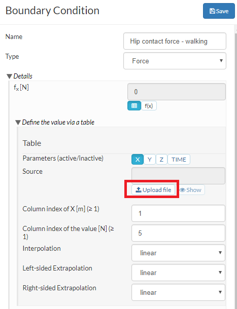
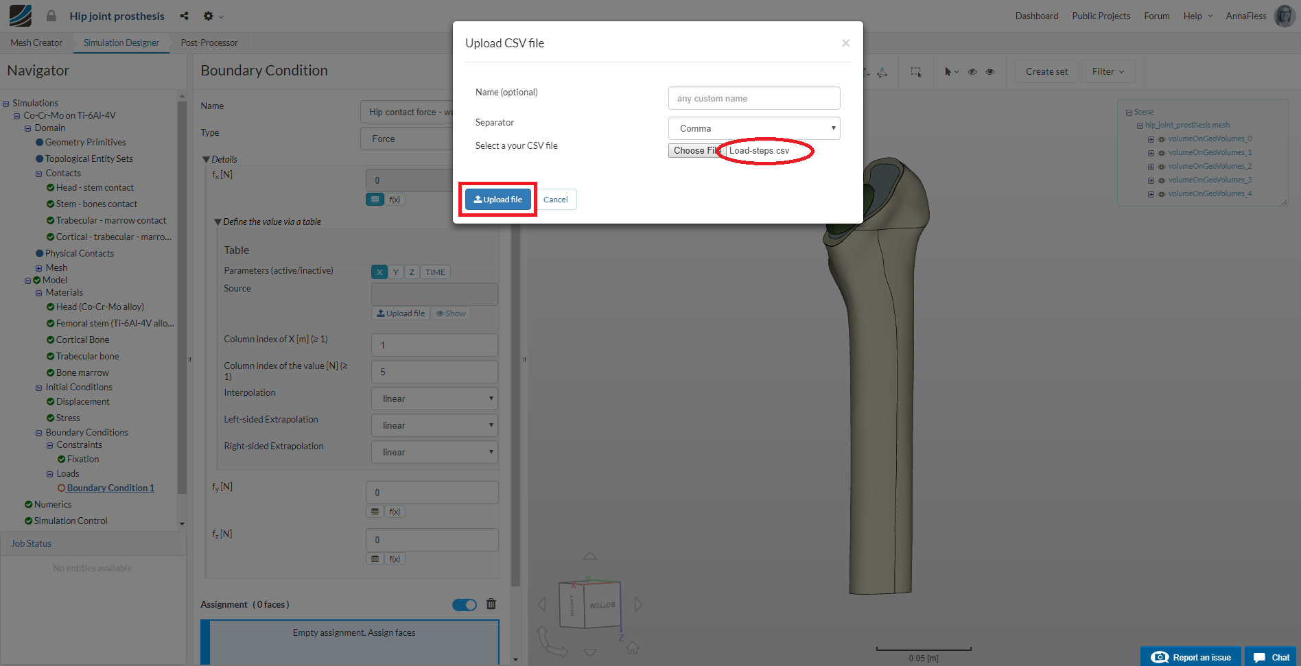
A pop-up will appear. Click on choose file and select the .csv file that you just downloaded. Then Upload file
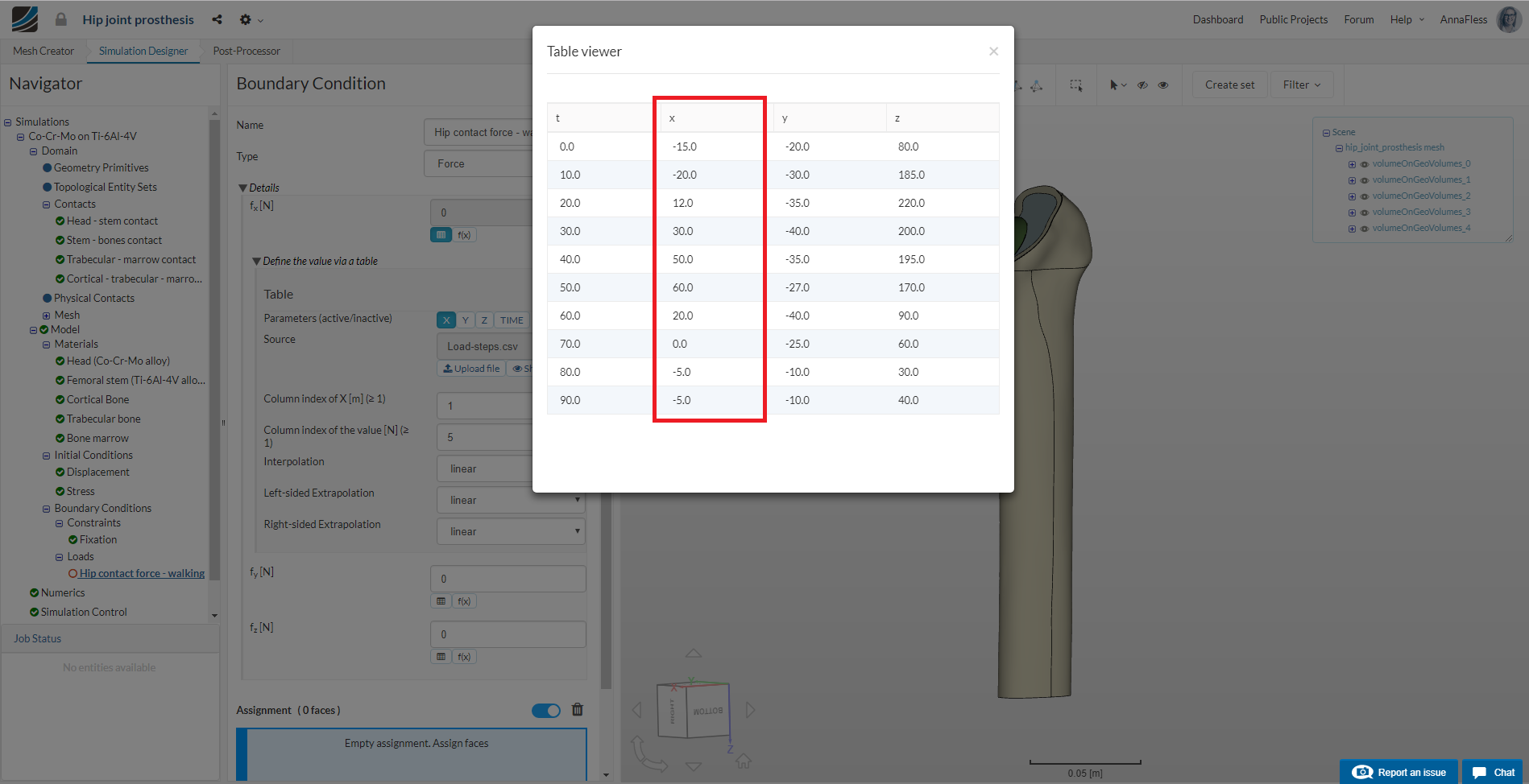
Click on Show to see the Table Viewer which contains the values. We need to make sure that the values for forces in the x-direction are selected.
Exit the Table Viewer and set Parameters (active/inactive) to Time.
Then set the Column index of Time [s] (≥ 1) to 1 and the Column index of the value [N] (≥ 1) to 2
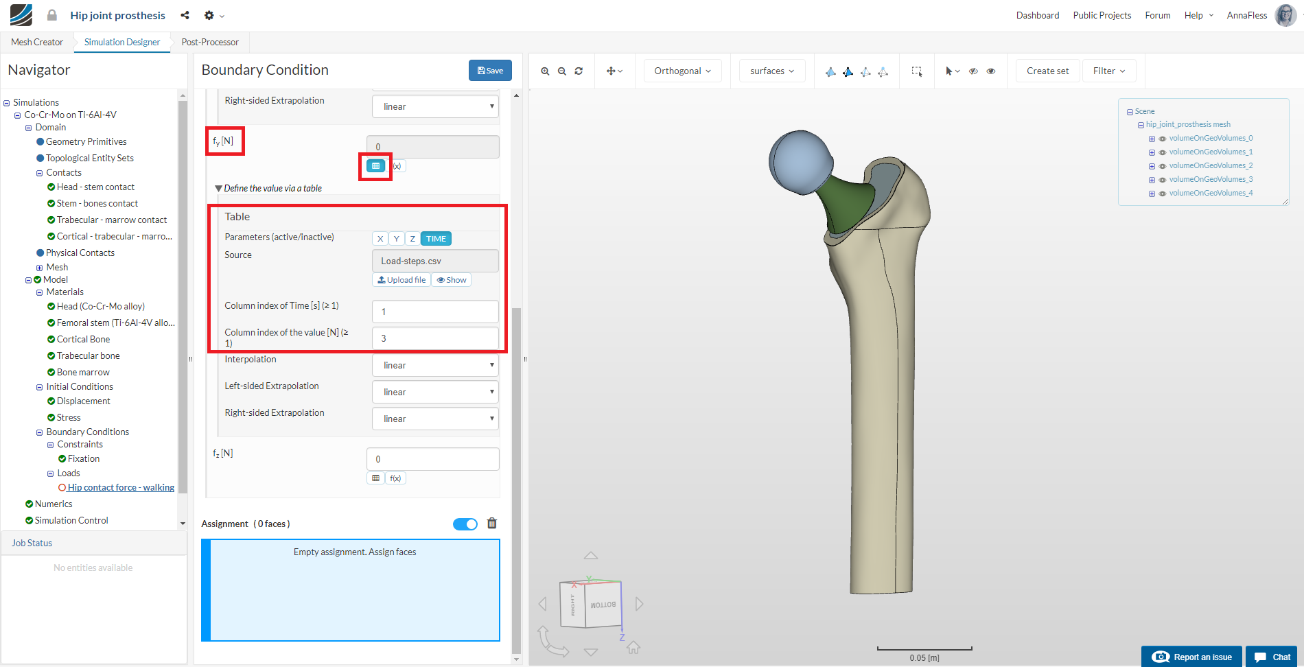
We need to follow the same steps for fy and fz.
Go to fy and click on the table upload icon. Again, upload the .csv file containing the forces for walking.
set Parameters (active/inactive) to Time.
Then set the Column index of Time [s] (≥ 1) to 1 and the Column index of the value [N] (≥ 1) to 3
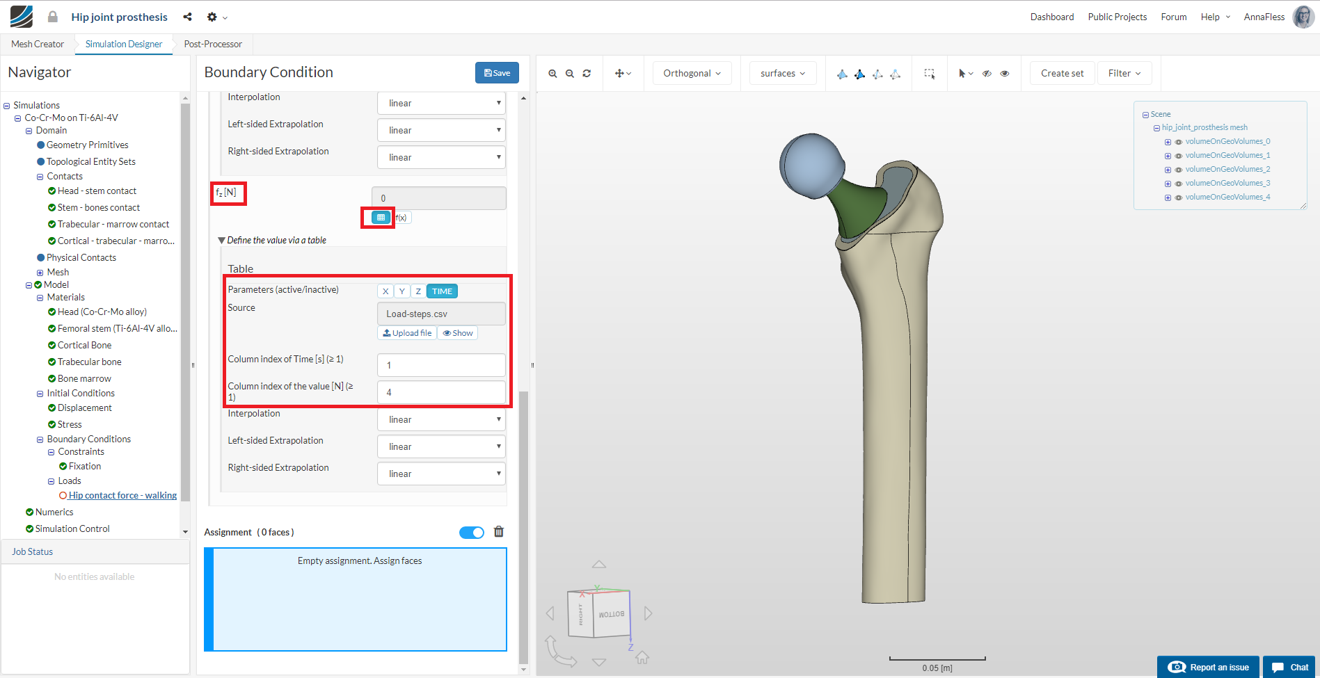
Finally go to fz and click on the table upload icon. Again, upload the .csv file containing the forces for walking.
set Parameters (active/inactive) to Time.
Then set the Column index of Time [s] (≥ 1) to 1 and the Column index of the value [N] (≥ 1) to 4
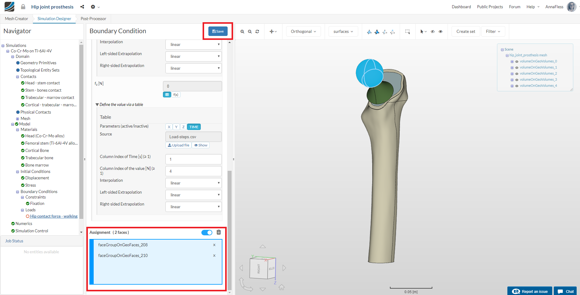
Select the top two faces of the hip joint head and then Save to save the constraint definition.
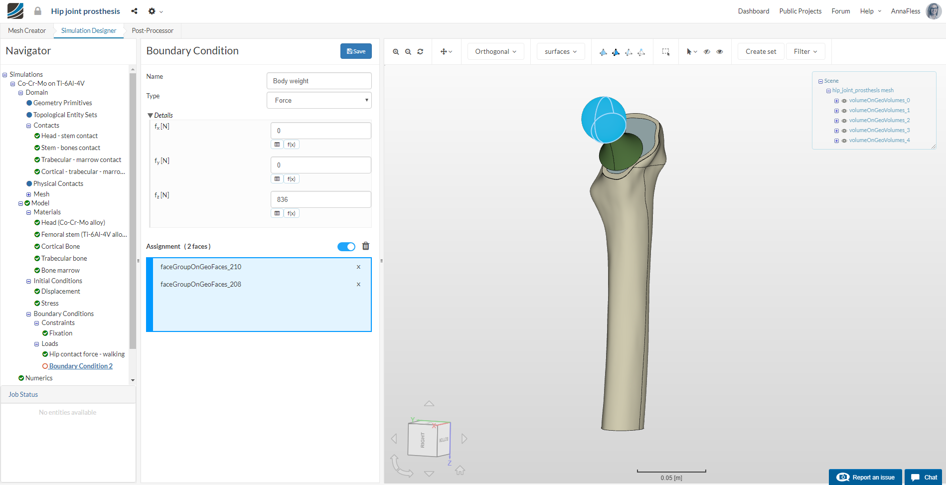
Load 2
Next we will define our body weight force to the top of the hip joint head. Create a new load.
Rename the newly created load to Body weight (optional). Select Force as the Type.
Change fx, fy and fz to 0, 0, 836 respectively.
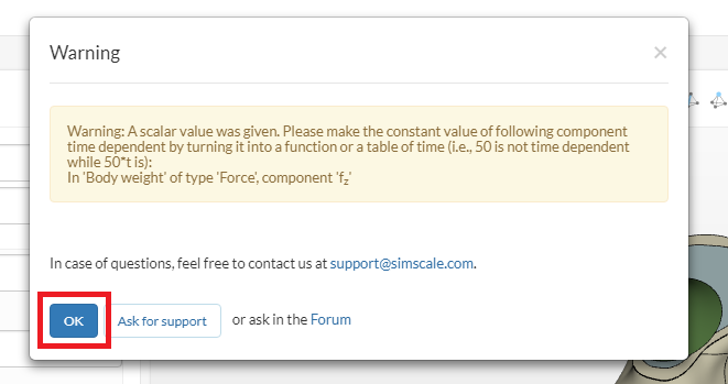
Select the top two faces of the hip joint head and then Save to save the constraint definition.
In case you get an ‘Warning’, select ok. We do not want to apply body weight as a function of time in this case.
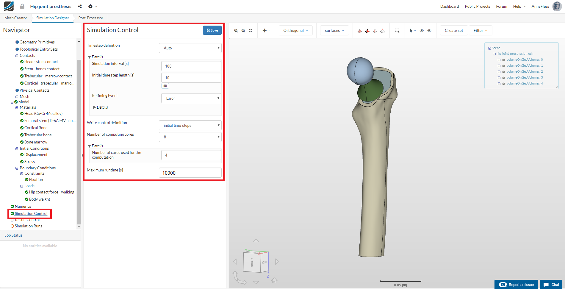
Simulation Control
Now go to the Simulation control item in the Navigator and expand the Details sections.
Set the Simulation interval [s] to 100 and the Initial time step length [s] to 10. This corresponds to the interval and time step length of the variable walking load that we uploaded.
Change the Number of computing cores to 8, the Number of cores used for the computation to 4, and the Maximum Runtime to 10000 seconds.
Click Save to register the changes.
Result Control
Next we will add the principal stress solution fields under Result Control which will let us see the maximum principal stresses in the simulation results. The maximum principal stresses will show the compressive stresses in our model, thus showing the stress shielding effect.
Go to Solution fields under Result Control and click on +New to add a new solution field.
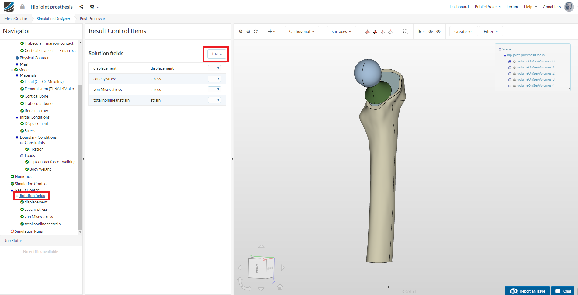
Rename the newly created solution field to principal stress (optional).
Select stress and principal stress as the Type and Stress type respectively. Click Save to save the solution field.

Simulation Run
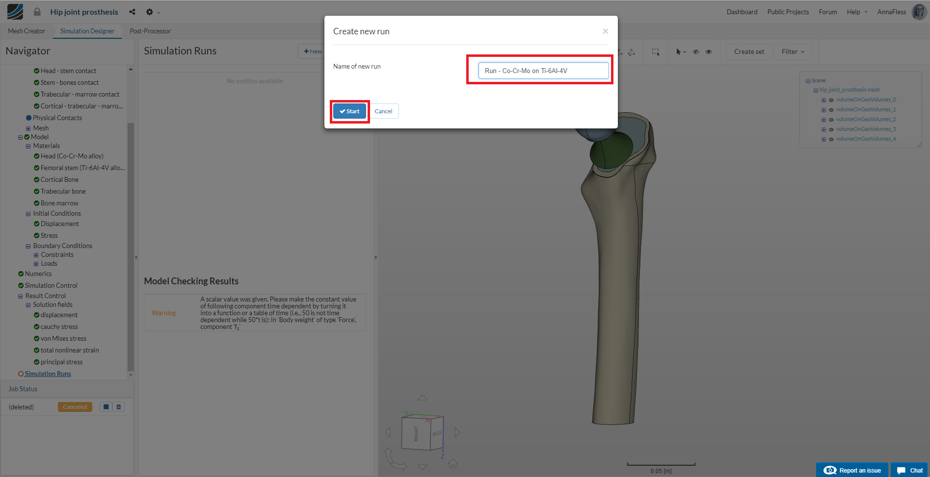
Now everything is done for setting up the first simulation run. Click on Simulation runs and create a new run. Again, you can ignore the Warning.
Give the simulation run a suitable name in the pop-up window that appears e.g. Run - Co-Cr-Mo on Ti-6Al-4V (optional) in this case.
Click Start to run the simulation.
The simulation run will take approx. 100 min. to finish. Now you can proceed to configurations 2 and configuration 3
Configuration 2:
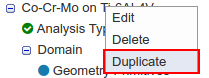
Once you have started the run with the first configuration setup, go ahead and make a duplicate of this simulation in order to perform the simulation with different material type for the hip joint (configuration 2).
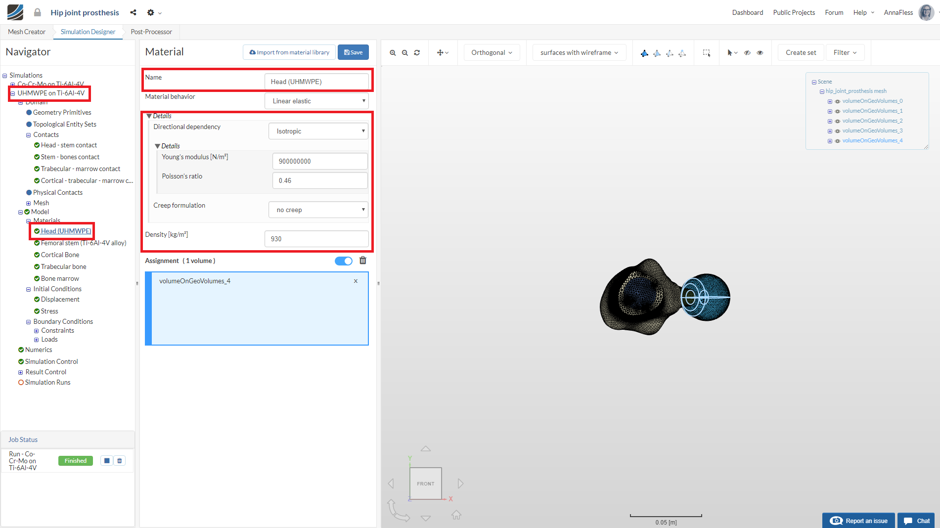
Rename the simulation to UHMWPE on Ti-6Al-4V.
All you need to do is to change the material definition of the femoral head to Ultra High Molecular Weight Polyethylene (UHMWPE).
Click on Head (Co-Cr-Mo alloy) under Materials, and rename it to Head (UHMWPE) (optional).
Change the Young’s modulus, Poisson’s ratio and Density values to 0.9e9, 0.46 and 930 as shown in the figure below. Click Save to save the material definition.
Next create a new simulation run, rename it to UHMWPE on Ti-6Al-4V (optional) and click Start to start the run.
Configuration 3:
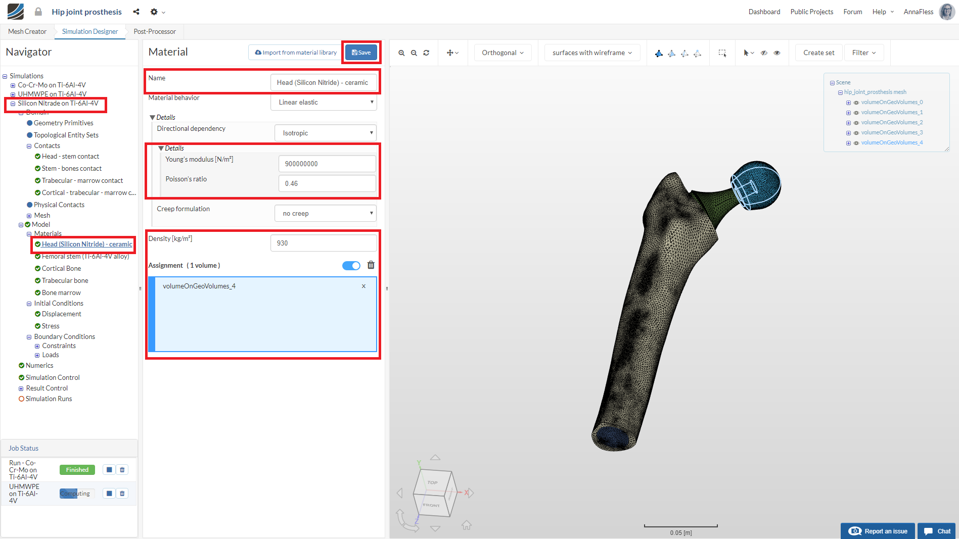
For Configuration 3, follow the same steps to duplicate the simulation and rename it to Silicon Nitride on Ti-6Al-4V (optional).
Click on Head (Co-Cr-Mo alloy) under Materials, and rename it to Head (Silicon Nitride) - ceramic (optional).
Change the Young’s modulus, Poisson’s ratio and Density values to 3.1e11, 0.26 and 3200 as shown in the figure below. Click Save to save the material definition.
Next create a new run, rename it to Silicon Nitride on Ti-6Al-4V (optional) and click Start to start the run.
If you are interested in seeing the effects on the hip joint for other materials, feel free to follow the same configuration steps to test your own material models
Post-processing
Once the simulation is over, click on Post-processor tab to view the results.
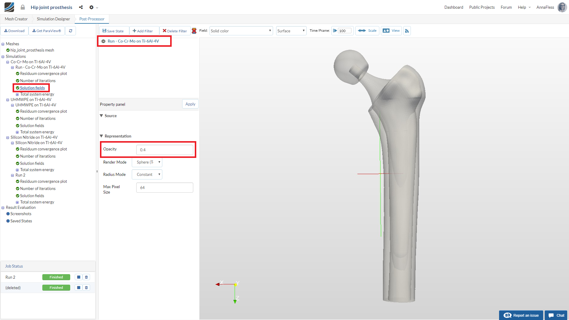
Select the Solution fields of the simulation run you want to view results. In this case it is Run-Co-Cr-Mo on Ti-6Al-4V.
Displacements
In order to differentiate between the deformed and undeformed geometry of the bone, change the field (at the top left corner) to Solid color and change the Opacity to 0.4 in the Property panel. This will make the bone transparent.
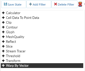
To see the deformed geometry, click on Add Filter and then Warp by Vector.
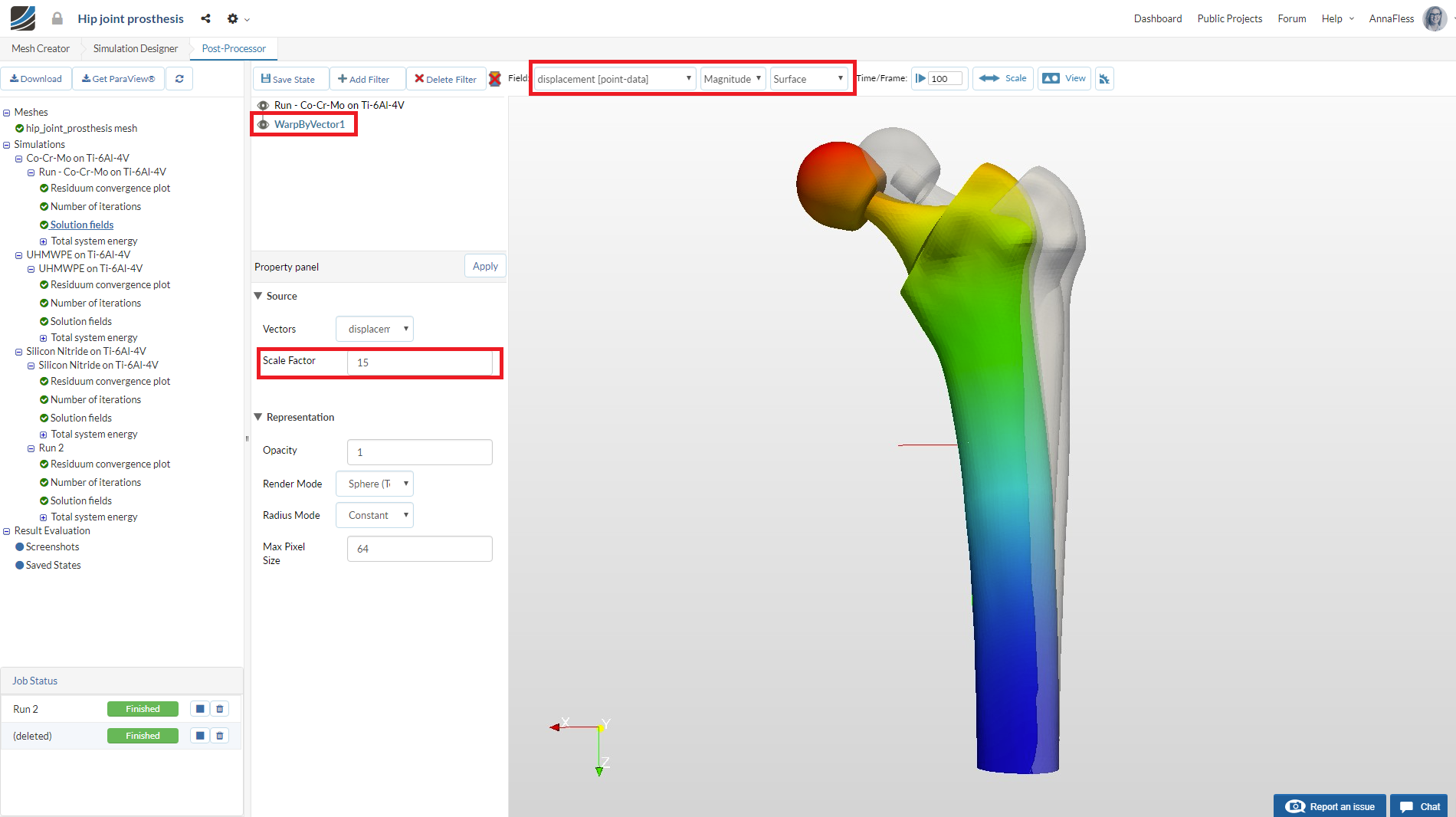
You will see a Warp by Vector filter is added under your solution field. Change the field to displacement to see the displacement values displayed.
Use a suitable scale factor to scale the deformed geometry, 15 in this case.
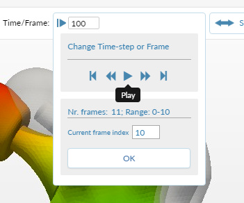
To see an animation, click the play button:
Stresses
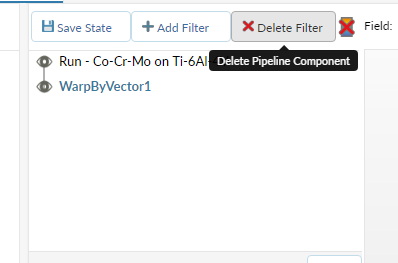
Click on WarpByVector1 and then Delete Filter. Then change the opacity of Run-Co-Cr-Mo on Ti-6Al-4V back to 1
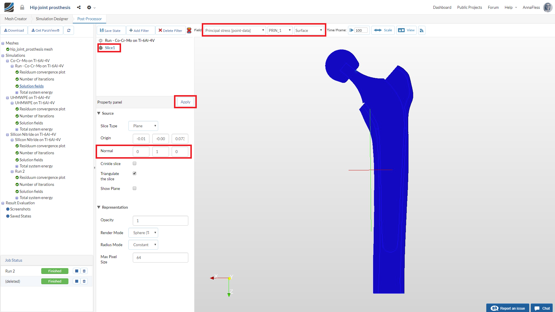
In order to view the stresses in the bone, we will add a slice filter. Click on Run-Co-Cr-Mo on Ti-6Al-4V.
Then click on Add Filter and select Slice. Change the Normal of the Slice to (0,1,0) and de-select Show Plane
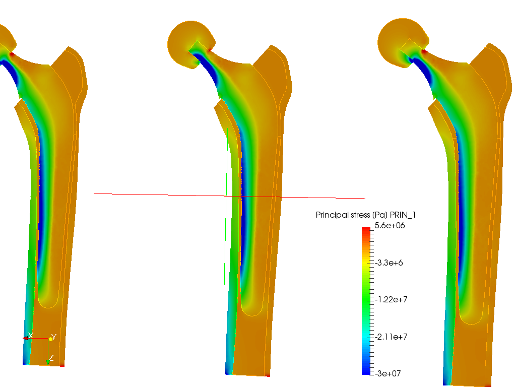
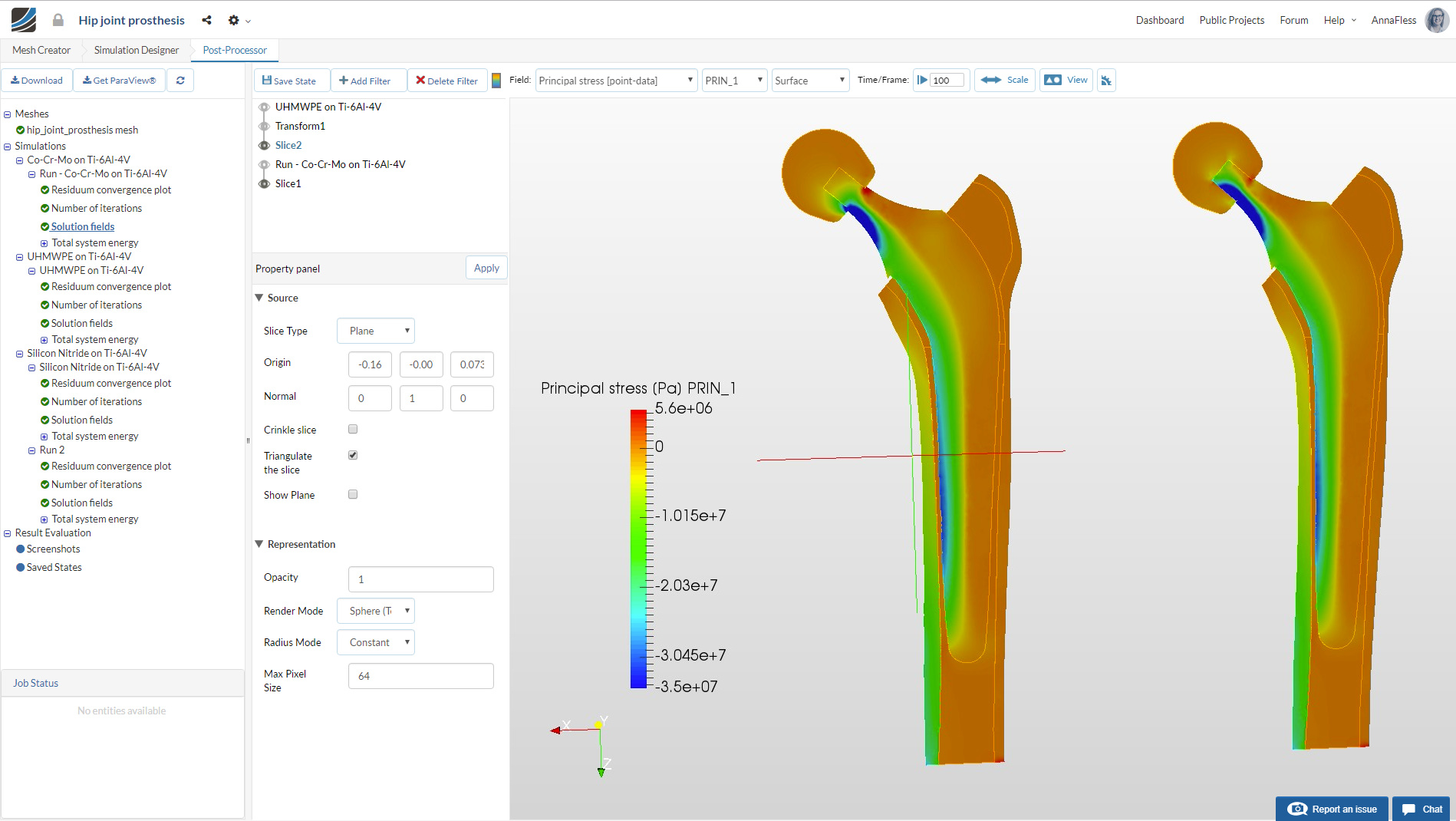
Change the field in the top viewer bar to Principal_stress and PRIN_1 (1st Principal Stress)
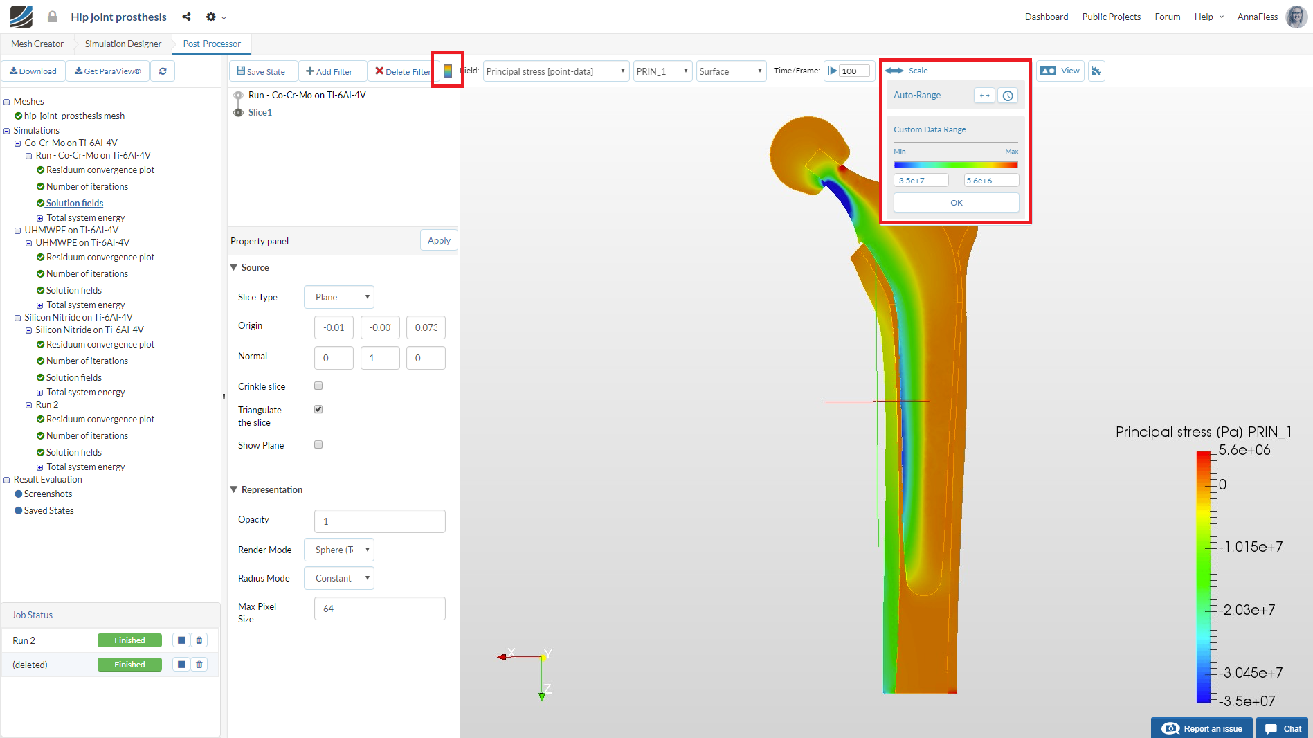
To view the better visualize the stresses, click on Scale and use the Auto-Range Option to scale the stresses or input the provided range: -3.5e7 and 5.6e6 Select the ruler to show the Stress values in the Viewer
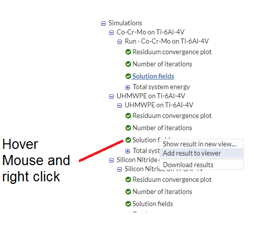
Now, we will load the results of UHMWPE on Ti-6Al-4V to the Viewer. HOVER your mouse over the Solution field item and RIGHT CLICK and choose Add results to viewer
The results are now overlapping so for viewing the results separately, we need to use the Transform filter.
Make sure UHMWPE on Ti-6Al-4V is selected
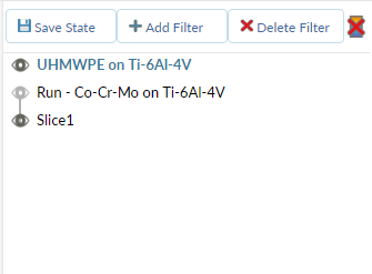
Now Add Filter and select Transform to move the results along the x-axis so that they have a gap of -0.15 meters between them by giving the value of -0.15 next to the Translate in the x-direction.
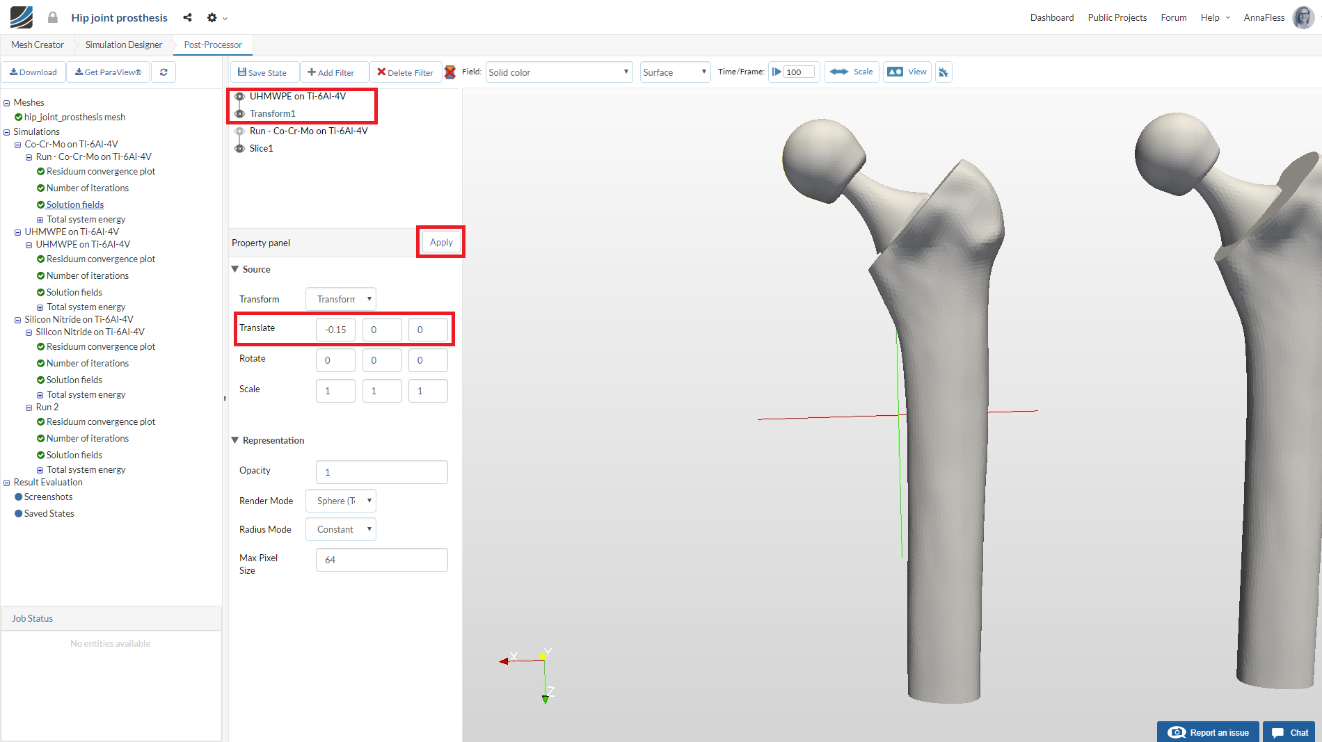
De-select the eye icon for UHMWPE on Ti-6Al-4V so you can only see the transformed solution
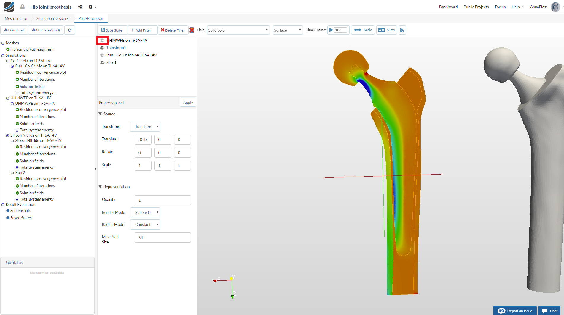
Now make sure Transform1 is highlighted in blue. Then click on Add Filter and select Slice. Change the Normal of the Slice to (0,1,0) and de-select Show Plane
Change the field in the top viewer bar to Principal_stress and PRIN_1 (1st Principal Stress)
To view the better visualize the stresses, click on Scale and use the Auto-Range Option to scale the stresses or input the provided range: -3.5e7 and 5.6e6 Select the ruler to show the Stress values in the Viewer.
Follow the same transformation procedure for the 3rd configuration results, Silicon Nitride on Ti-6Al-4V in this case. This time use Translate x-axis value of -0.3
In this workshop we are using maximum principal stress for comparison. The purpose of using this stress quantity to visualize the results is that it clearly shows the tension and compression regions (+ indicates tension and - indicates compression).
What observations can you make about the results? Which prosthesis would you choose and why?
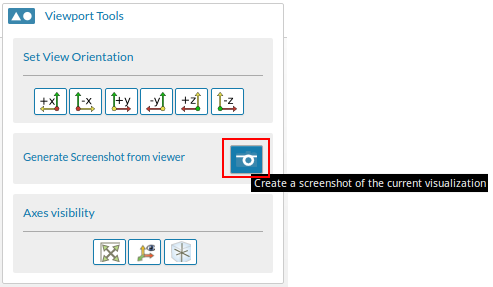
You can save post-processing screenshot by clicking on camera icon under Viewport Tools. The screenshot will appear under Screenshots section of a Result Evaluation tree item.
References
[1] K. Chalernpon, P. Aroonjarattham, K. Aroonjarattham, et al. “Static and Dynamic Load on Hip Contact of Hip
Prosthesis and Thai Femoral Bones” International Journal of Mechanical and Mechatronics Engineering
Vol:9, No:3, 2015
[2] The base model for the femur bone used in this exercise is provided by Negar An from GrabCAD