Step-by-Step Tutorial: Homework of Session 3

[Akrem]

Recording

Formula Student / Formula SAE Workshop: Development Strategies

Homework Submission

Submitting all four homework assignments will qualify you for a free Professional Training (value of 500€) as well as a SimScale Certificate of Completion.

Homework 3 - Deadline: Date, 22nd of December, 11:59 pm

[Homework Submission Form] (Simulation Software | Engineering in the Cloud | SimScale)

Introduction

In this exercise we will investigate the effects of side wind on the performance of the car. Your task is to investigate the full car model Model-Conf-Yaw. The velocity of the car will be considered constant at 20 m/s with side wind.

To start this exercise, please import the project into your workspace by clicking on the link below:

SimScale Login

Mesh Generation

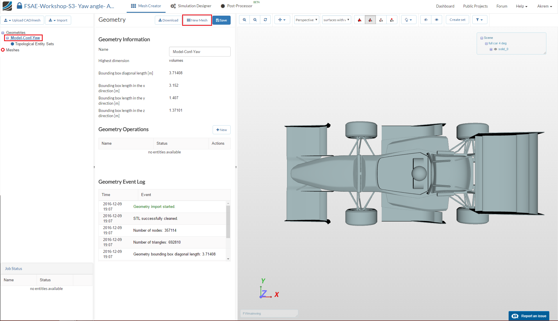
In the Mesh Creator tab, click on the geometry Model-Conf-Yaw

Click on the New Mesh button

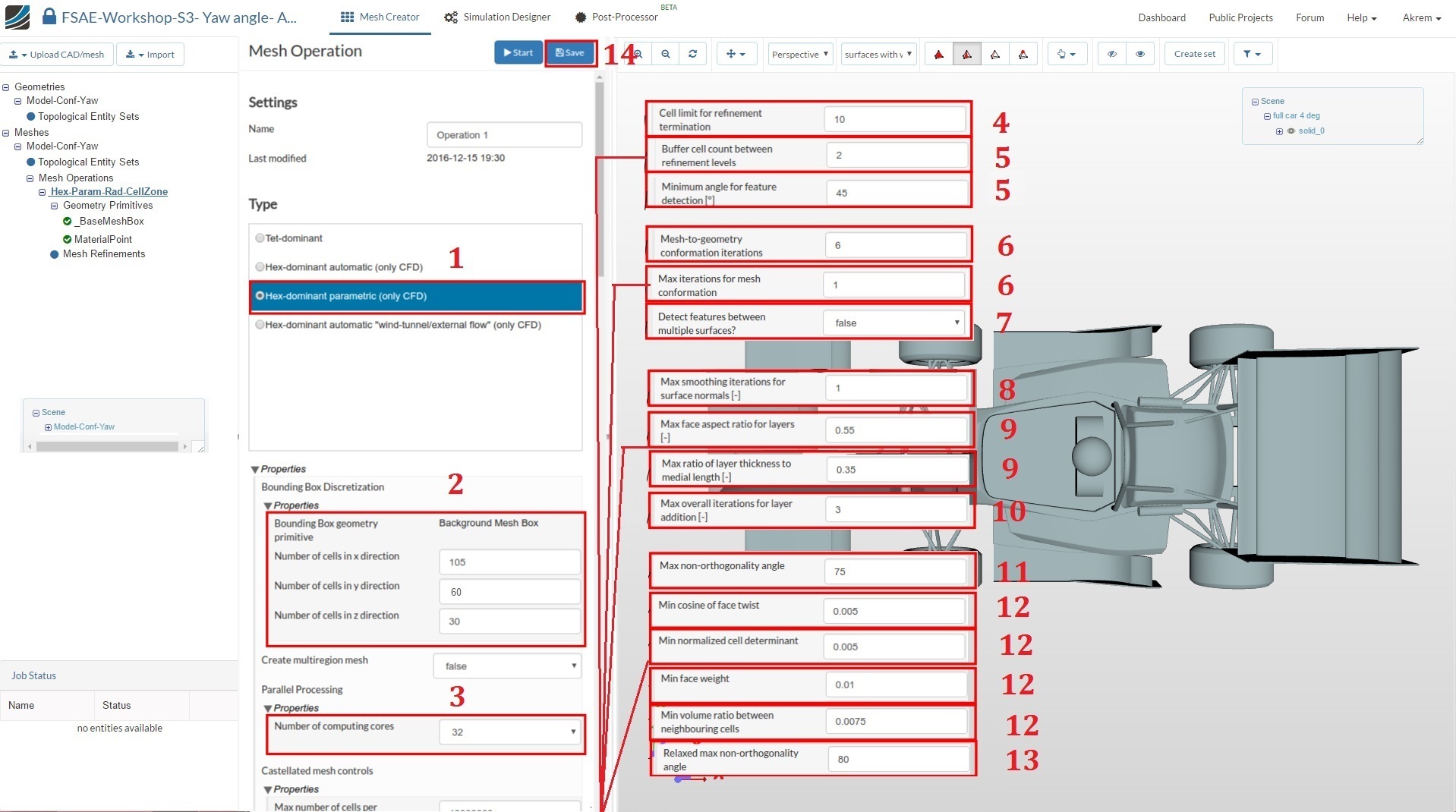
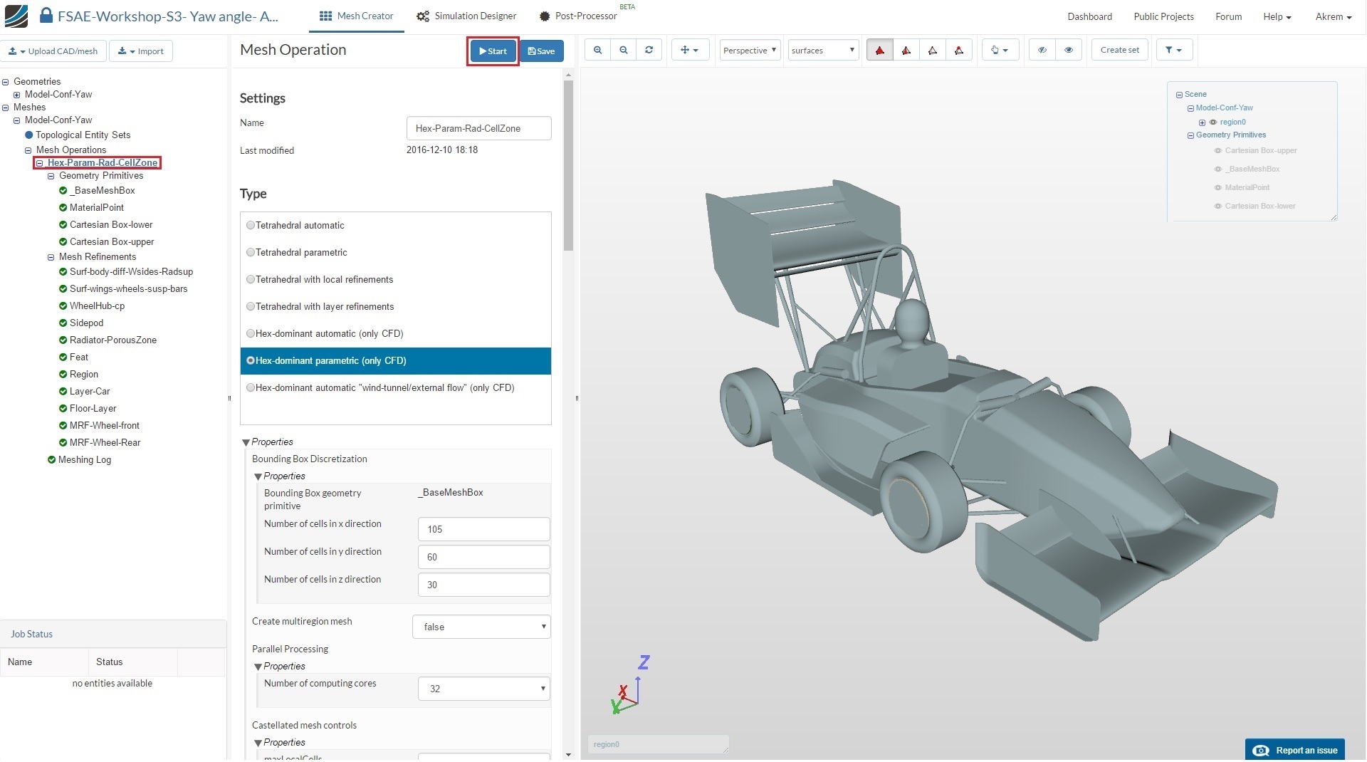
A new mesh operation will be generated automatically. Next change:

1. Type to Hex-dominant parametric (only CFD)

2. Bounding Box geometry primitive to the following:
   Number of cells in x direction to 105
   Number of cells in y direction to 60
   Number of cells in z direction to 30

3. Number of parallel computing cores to 32 [Scroll down to change other values to optimize the meshing parameters]

4. Cell limit for refinement termination to 10

5. Buffer cell count between refinement levels and Minimum angle for feature detection [°] to 2 and 45 respectively

6. Mesh-to-geometry conformation iterations to 6 and Max iterations for mesh conformation to 1

7. Detect features between levels to false

8. Max smoothing iterations for surface normals [-] to 1

9. Max face aspect ratio for layers [-] and Max ratio of layer thickness to medial length [-] to 0.55 and 0.35 respectively

10. Max overall iterations for layer addition to 3

11. Max non-orthogonality angle to 75

12. Min cosine for face twist, Min normalized cell determinant,Min face weight and Min volume ratio between neighbouring cells to 0.005, 0.005, 0.01 and 0.0075 respectively

13. Relaxed max non-orthogonality angle to 80

14. Click Save to register changes.

Background Mesh Box

Next go to the Background Mesh Box item and change the mesh box dimensions to the values shown in figure below. Click Save to save the changes.

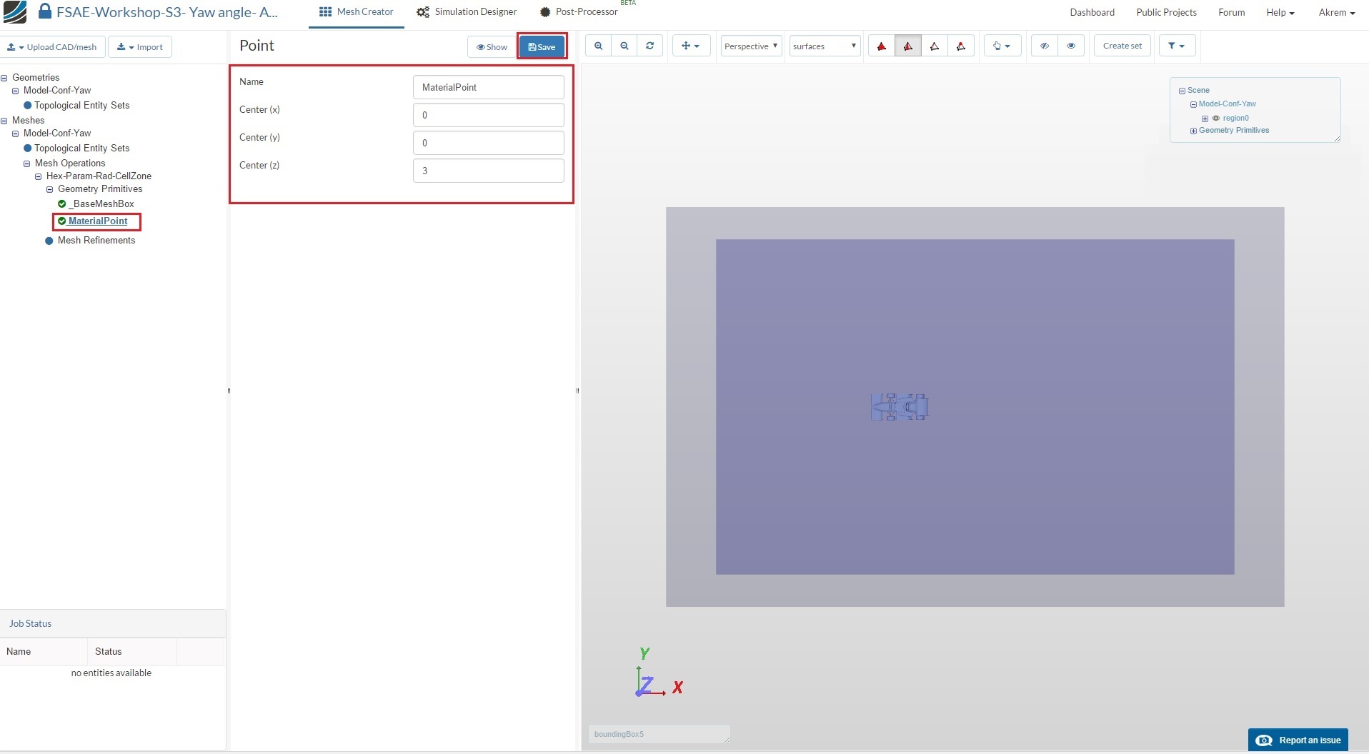
Material Point

Go to the MaterialPoint item and change the values to those shown in the figure below. Click Save to save the changes.

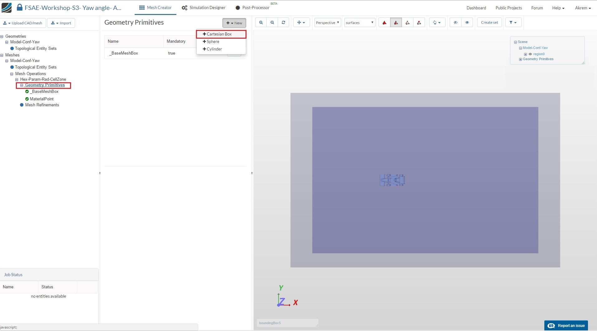
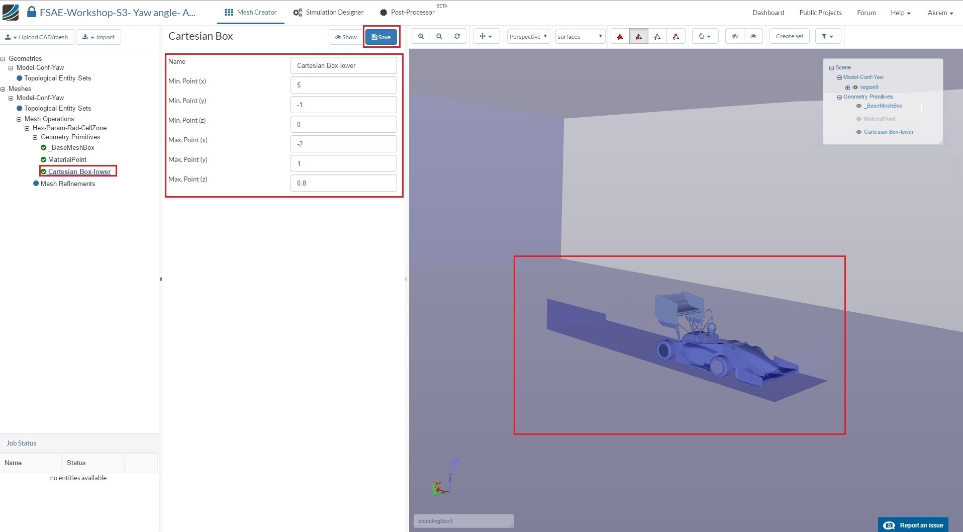
Cartesian Box-lower

Next go back to Geometry Primitives and click on +New and then Cartesian Box to define a new Cartesian box that will be used to define mesh refinement area.

After creating a new cartesian box, you will be directed to the definition of this cartesian box. Rename it to Cartesian Box-lower (optional) and change the dimensions to those shown in the figure below. Click Save to register your changes.

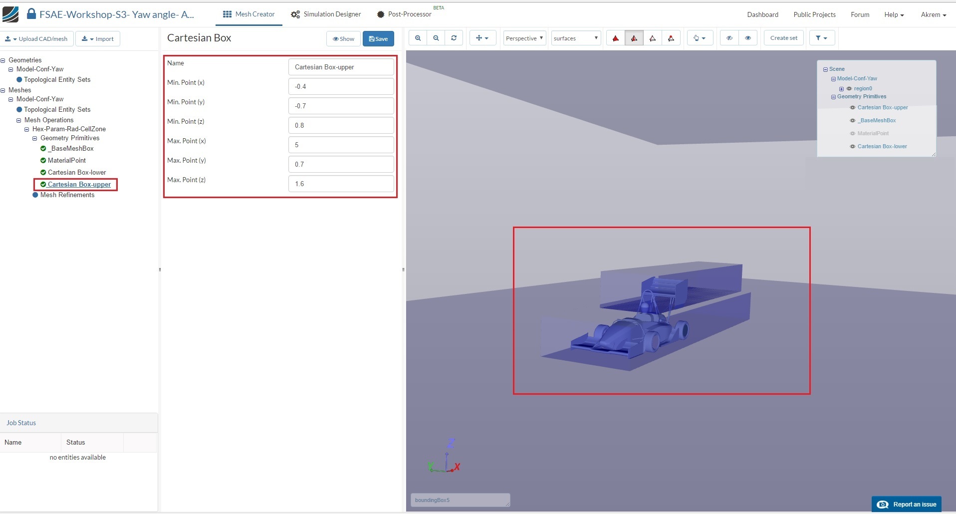
Cartesian Box-upper

Follow the same procedure to create a second cartesian box geometry primitive. Rename it to Cartesian Box-upper (optional). This time change the dimensions to those shown in the figure below. Click Save to register your changes.

Now we will start creating the mesh refinements. For this proceed to Mesh Refinements and click +New

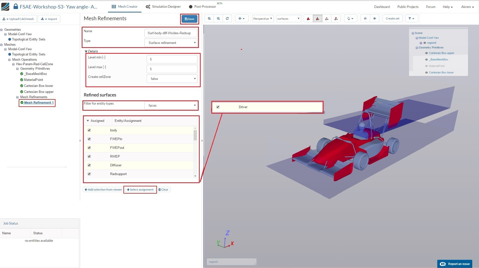
Mesh Refinement 1

A new mesh refinement will be created. Rename it to Surf-body-diff-Wsides-Radsup (optional).

Change the Type to Surface refinement

Set Level min and Level max to 5 and 5 respectively.

Change Filter for entity types to faces and select body, FWEPin, FWEPout, RWEP, Diffuser, Radsupport and Driver. Click Select assignment in order to see the selected assignments highlighted in the viewer.

Click Save to register your changes.

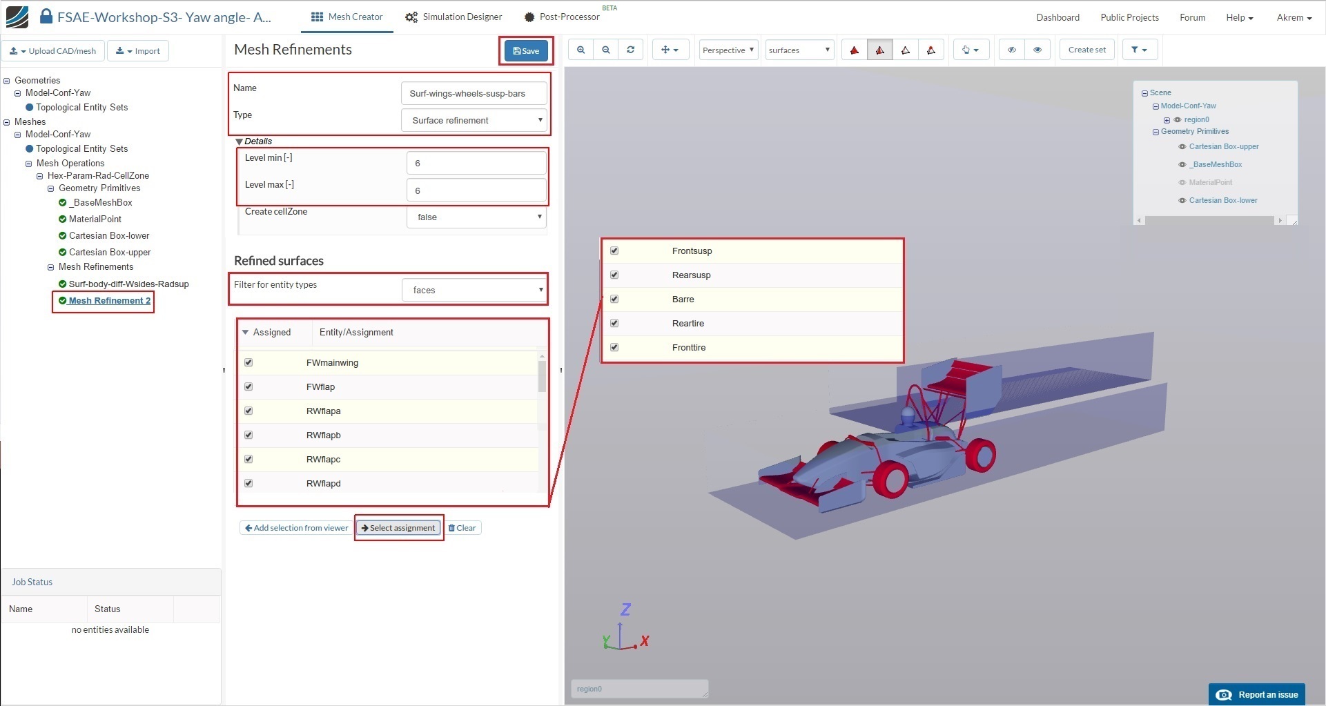
Mesh Refinement 2

Follow the same procedure and create a new mesh refinement named Surf-wings-wheels-susp-bars (optional).

Change the Type to Surface refinement

Set Level min and Level max to 6 and 6 respectively.

Change Filter for entity types to faces and select FWmainwing, FWflap, RWflapa, RWflapb, RWflapc, RWflapd, Frontsusp, Rearsusp, Barre, Reartire and Fronttire. Click Select assignment in order to see the selected assignment highlighted in the viewer.

Click Save to register your changes.

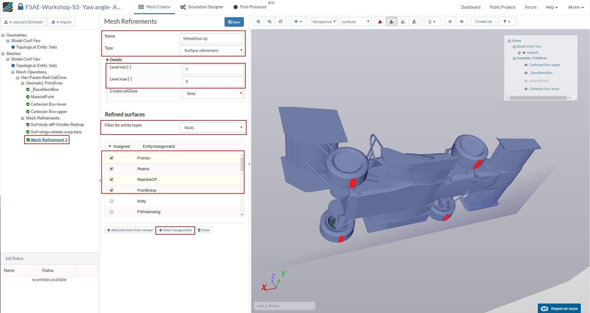
Mesh Refinement 3

Create a new mesh refinement named WheelHub-cp (optional).

Change the Type to Surface refinement

Set Level min and Level max to 7 and 8 respectively.

Change Filter for entity types to faces and select Frontur, Rearur, ReartireCP and Fronttirecp. Click Select assignment in order to see the selected assignment highlighted in the viewer.

Click Save to register your changes.

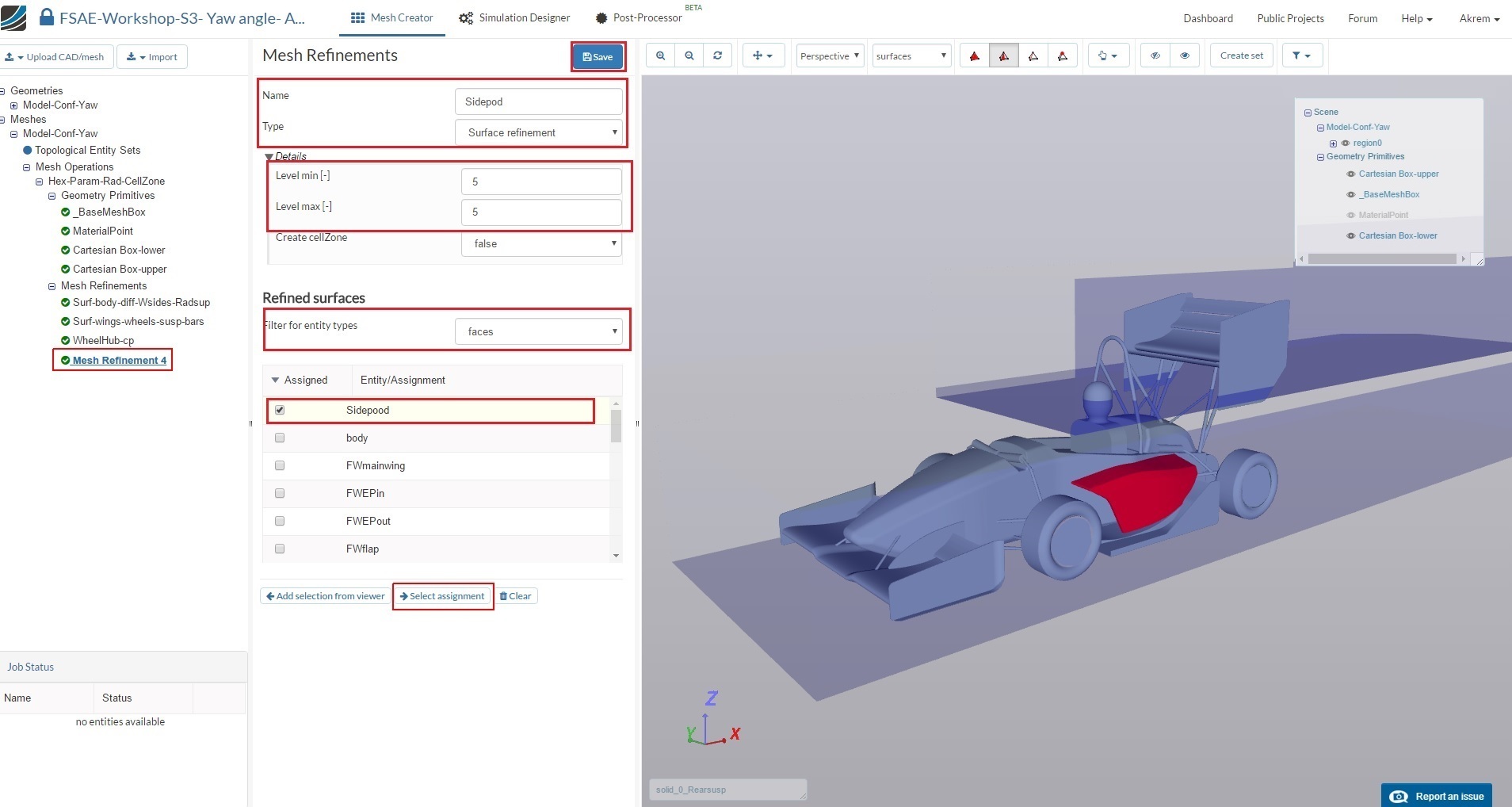
Mesh Refinement 4

Create a new mesh refinement named Sidepod (optional).

Change the Type to Surface refinement

Set Level min and Level max to 5 and 5 respectively.

Change Filter for entity types to faces and select Sidepod. Click Select assignment in order to see the selected assignment highlighted in the viewer.

Click Save to register your changes.

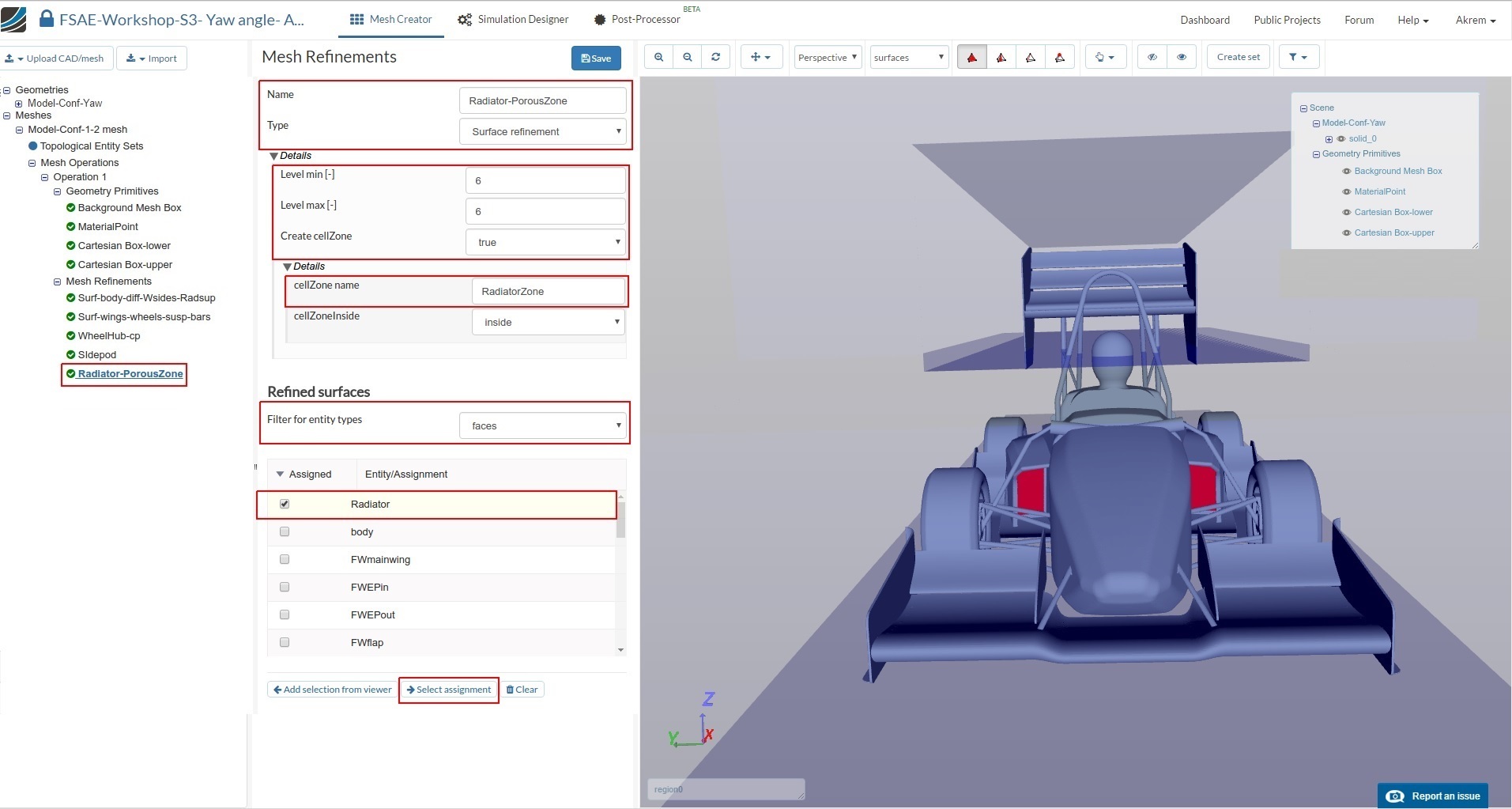
Mesh Refinement 5

Create a new mesh refinement named Radiator-PorousZone (optional).

Change the Type to Surface refinement

Set Level min and Level max to 6 and 6 respectively.

Set Create cellZone to true and rename cellZone name to RadiatorZone.

Change Filter for entity types to faces and select Radiator. Click Select assignment in order to see the selected assignment highlighted in the viewer.

Click Save to register your changes.

Mesh Refinement 6

In order to create a separate feature refinement for small features, create a new mesh refinement named Feat (optional).

Change the Type to Feature refinement

Then click the + button to add an extra value. In the first row, change Distance and Level value to 0.0015 and 8 respectively. Similarly, change the value to 0.005 and 6 in second row.

Click Save to register your changes.

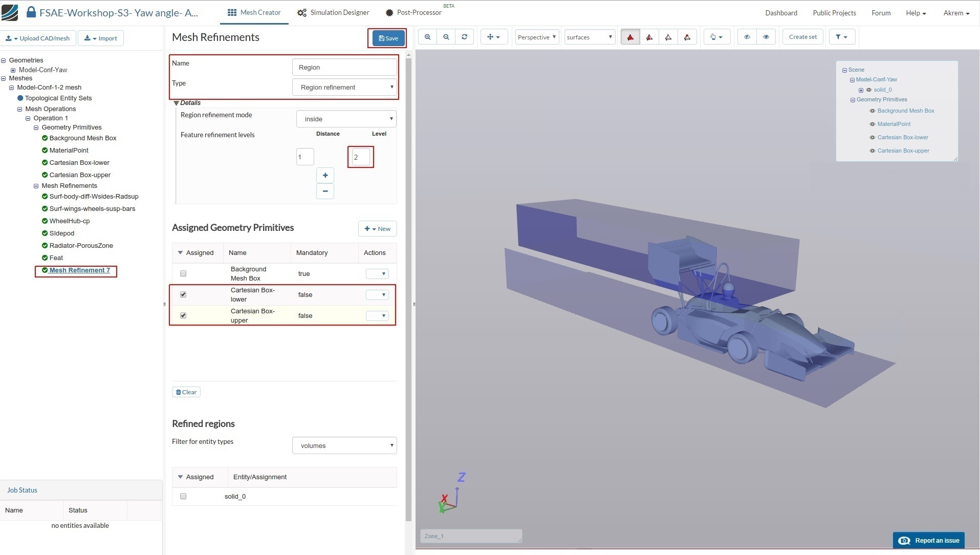
Mesh Refinement 7

To define the refinement level for the created cartesian box geometry primitives, create a new refinement and rename it to Region (optional).

Change the Type to Region refinement and set the level to 2

Select Cartesian Box-inner and Cartesian Box-outer under Assigned Geometry Primitives

Click Save to register the refinements for the specific cartesian boxes.

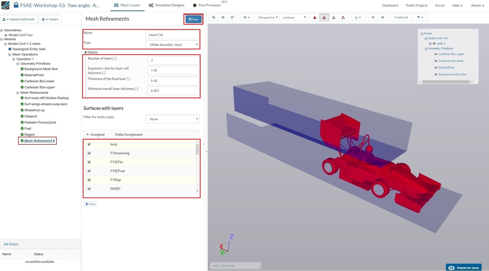
Mesh Refinement 8

Next we will define layers over the car surfaces in order to capture the results more accurately within the areas we are interested in.

Create a new refinement and rename it to Layer-Car (optional).

Change the Type to Inflate boundary layer

Then change Number of layers [-], expansionRatio [-], finalLayerThickness [-] and minThickness [-] to 3 , 1.05, 0.45 and 0.001 respectively.

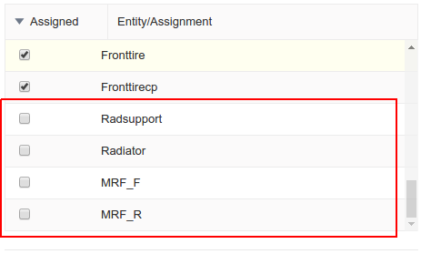
Select all the faces except Radiator, Radsupport, MRF_F and MRF_R under Surfaces with layers and click Select assignment in order to review the selected surfaces in the viewer.

Click Save to register your changes.

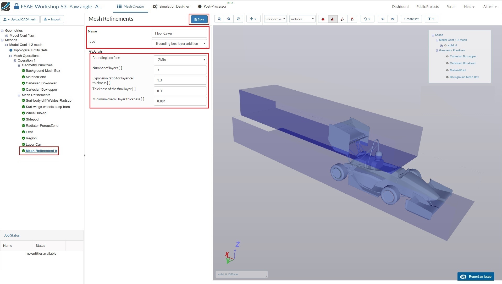
Mesh Refinement 9

For the floor layers, create a new refinement named Floor-layer (optional).

Change the Type to Boundary box layer addition.

Change Bounding box face to Zmin and then the Number of layers and MinThickness to 3 and 0.001 respectively.

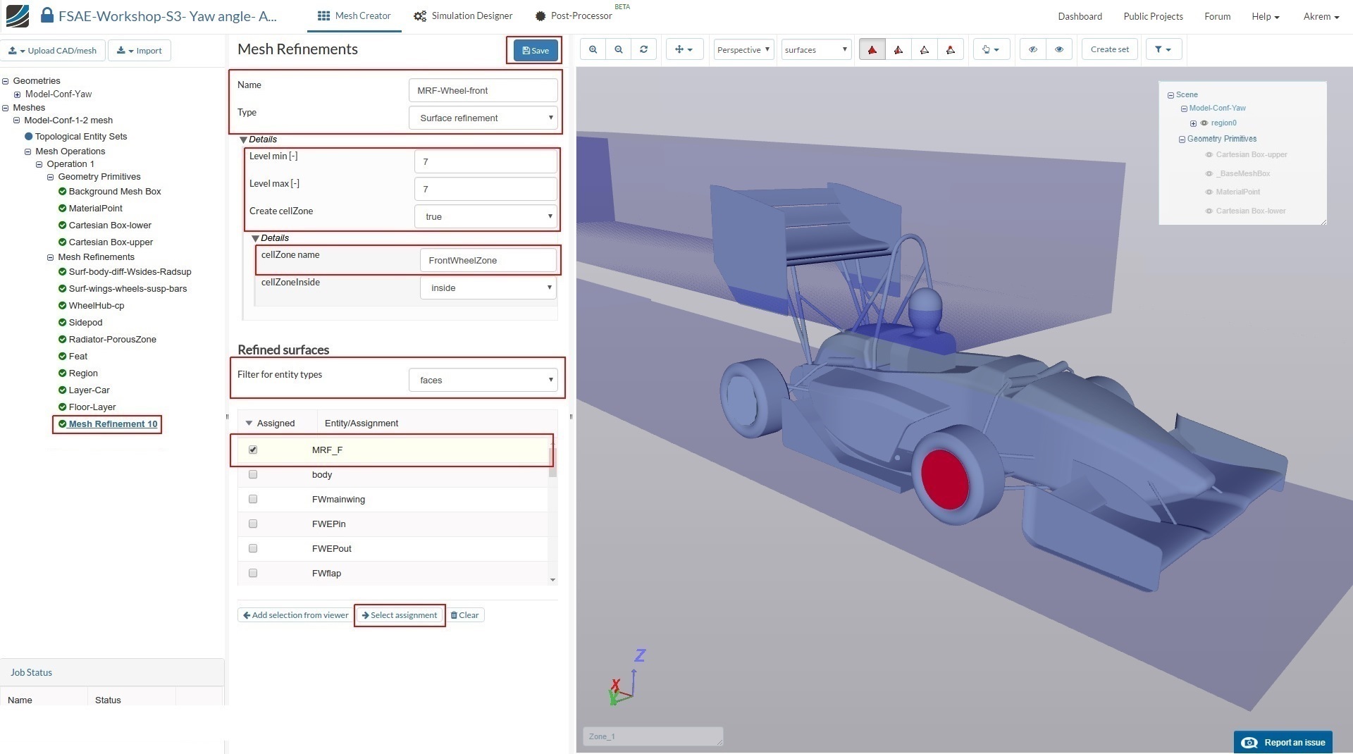
Mesh Refinement 10

Create a new refinement for the front MRF zone named MRF-Wheel-front (optional).

Change Type to Surface refinement

Set Level min and Level max to 7 respectively.

Change Create cellZone to true and rename cellZone name to FrontWheelZone.

Change Filter for entity types to faces and select MRF_F

Click Save to register your changes.

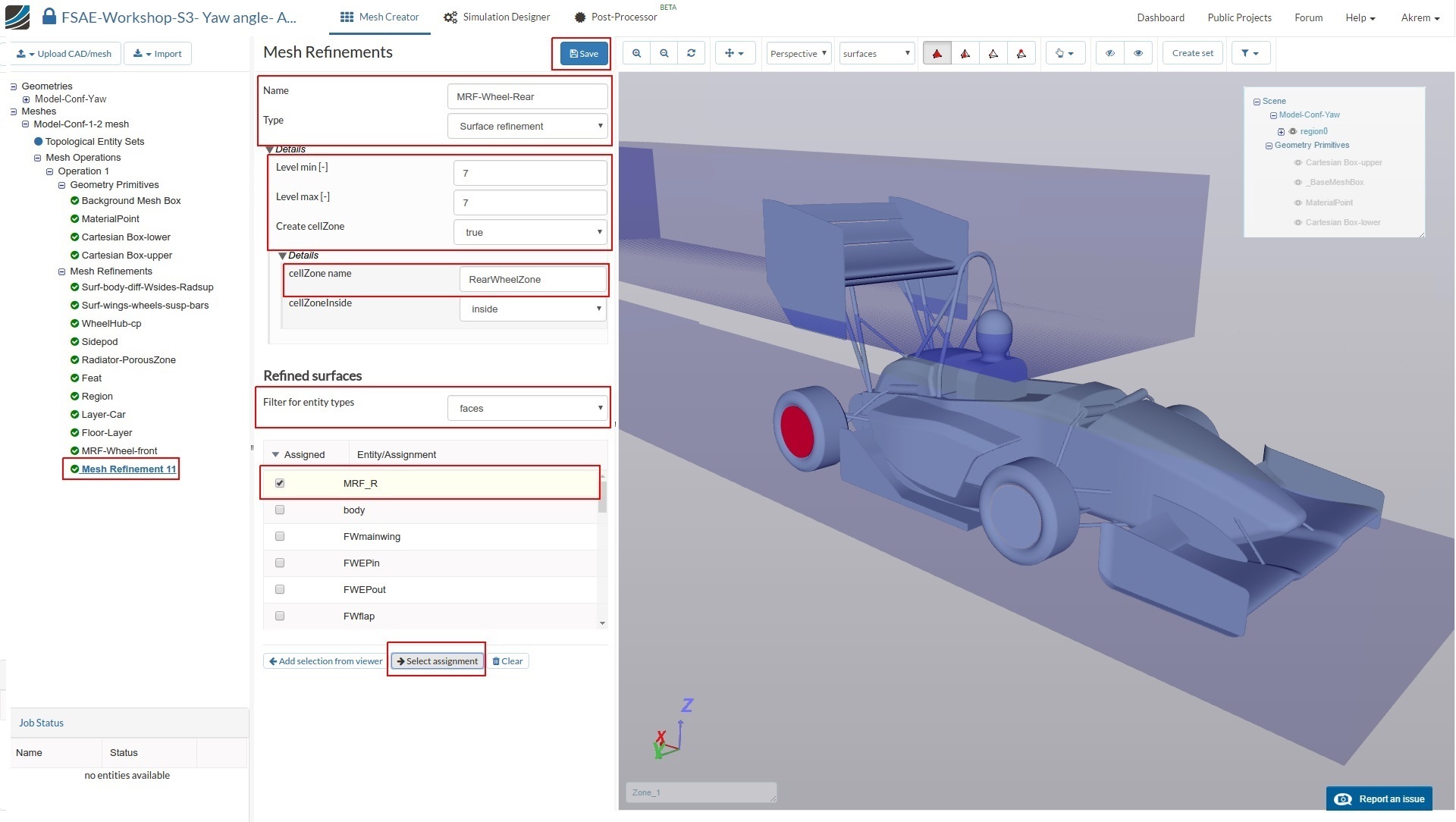
Mesh Refinement 11

Similarly, for rear MRF zone create a new refinement named MRF-Wheel-Rear (optional).

Change the Type to Surface refinement

Set both Level min and Level max to 7 respectively.

Change Create cellZone to true and rename cellZone name to RearWheelZone.

Change Filter for entity types to faces and select MRF_R.

Click Save to register your changes.

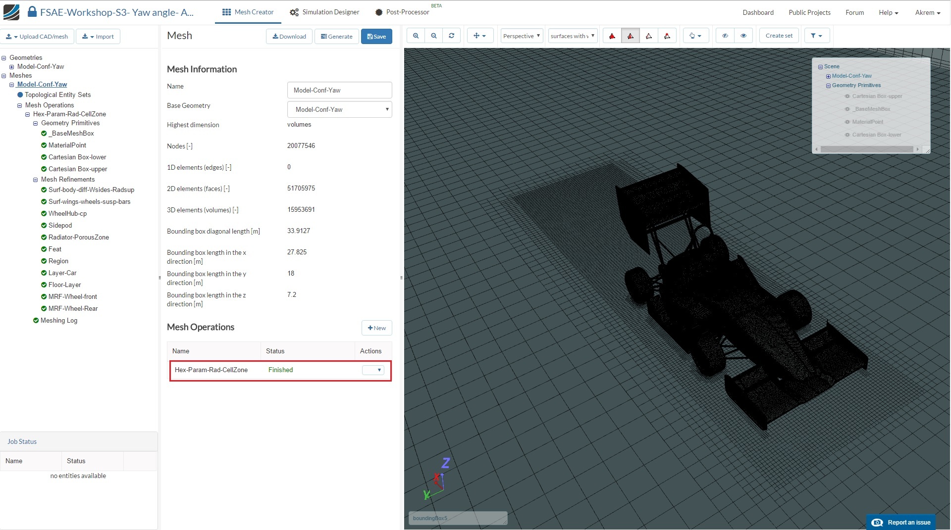
Once you have defined all 11 of the mesh refinements, go back to the Operation 1 and click Start.

Due to the fineness of the mesh, the meshing operation can take 100 to 140 minutes to finish.

Simulation

Once the meshing operation is complete, go to the Simulation Designer

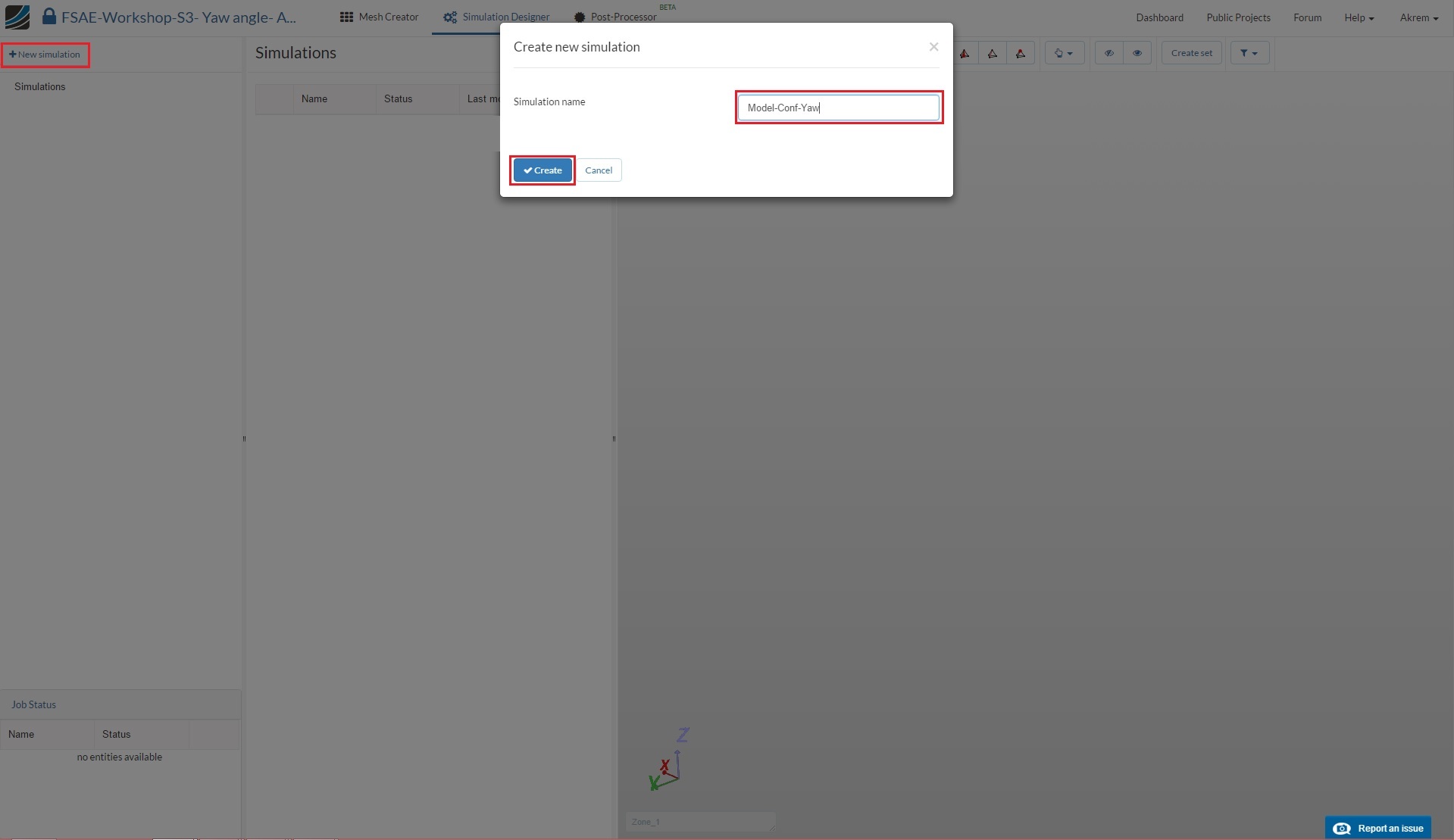
Click New Simulation and name it Conf-Yaw (optional; you can choose any name you want). Then click Create.

Analysis type

Under Analysis Type, switch to Fluid dynamics and then select Incompressible. You don’t have to change any other properties here.

Click Save

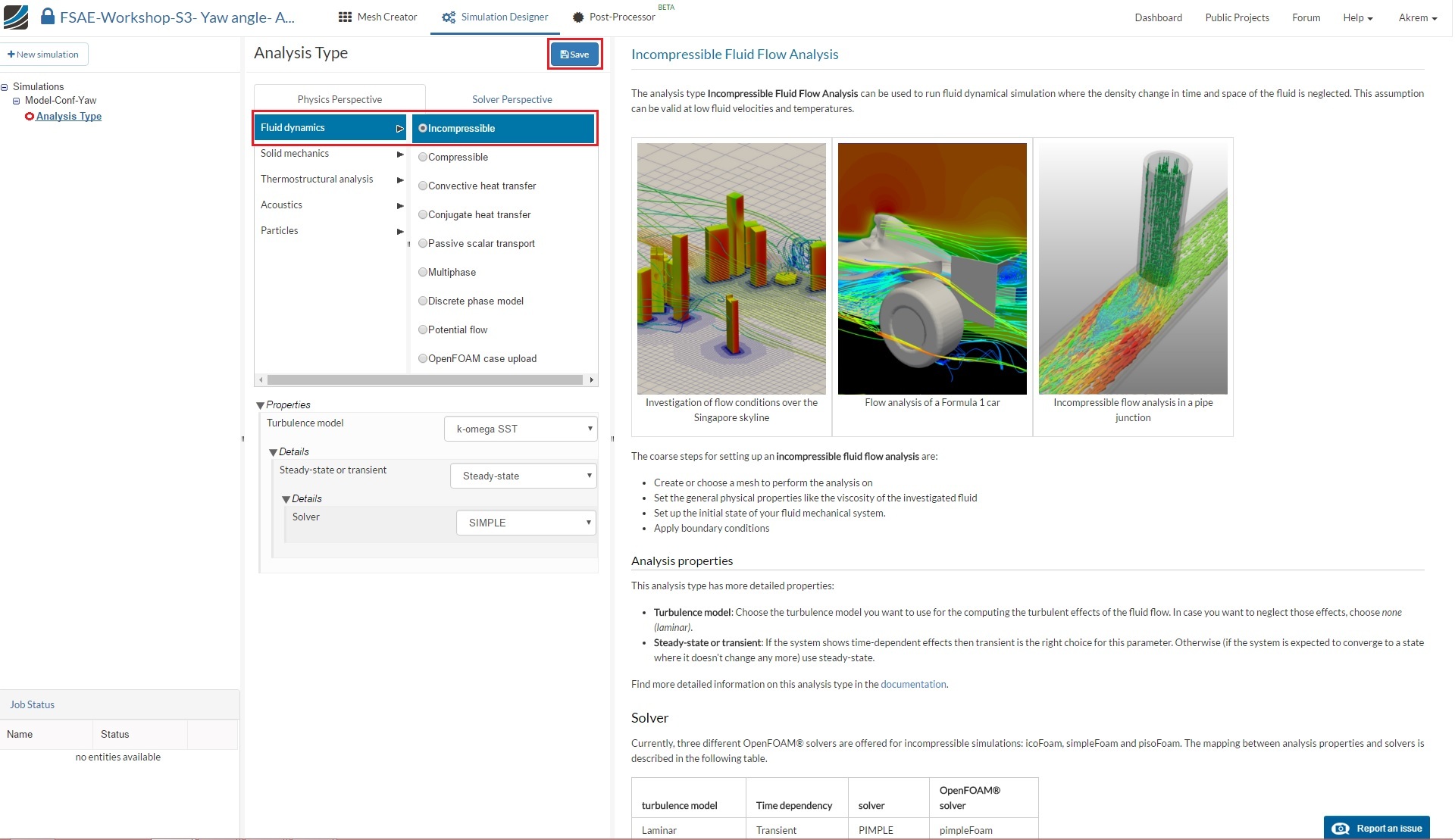
Once you save the analysis type, the items in the Navigator will expand. All of the red entities must be set up in order to perform a successful simulation run.

Domain

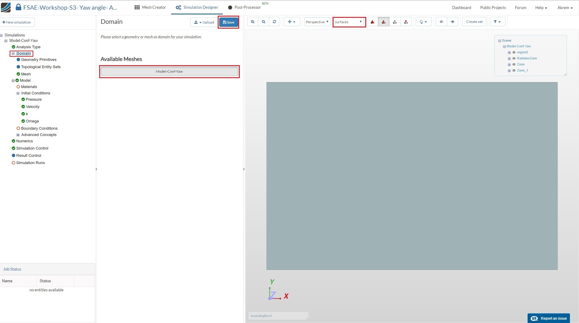
Proceed to the Domain item in the Navigator and select the mesh you just created. Then click Save. You will see the loaded mesh of the selected domain in the viewer. For the easier mesh handling, it is recommended to switch to the surfaces render mode in the top viewer bar.

Material

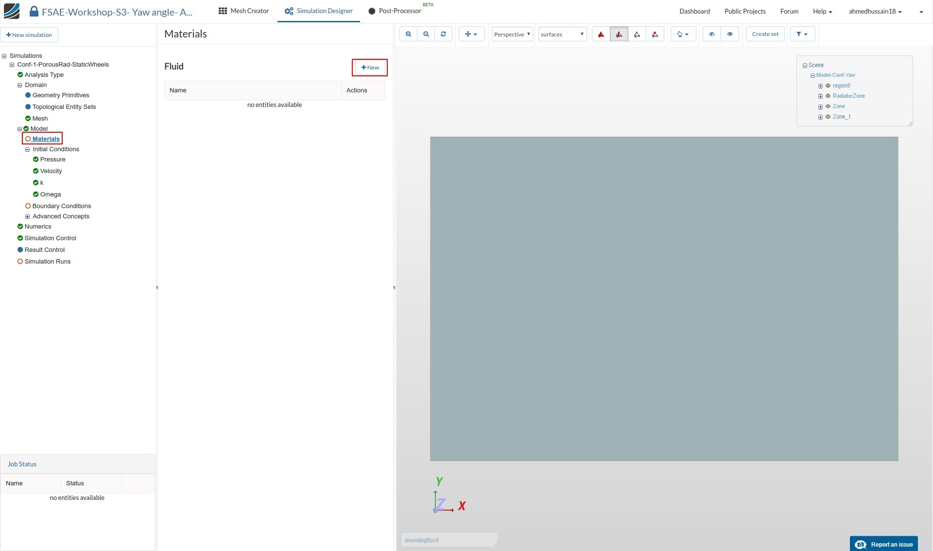
Next we have to define the fluid material. Go to Materials and click on +New

Click on Import from material library to import the desired material from the material database.

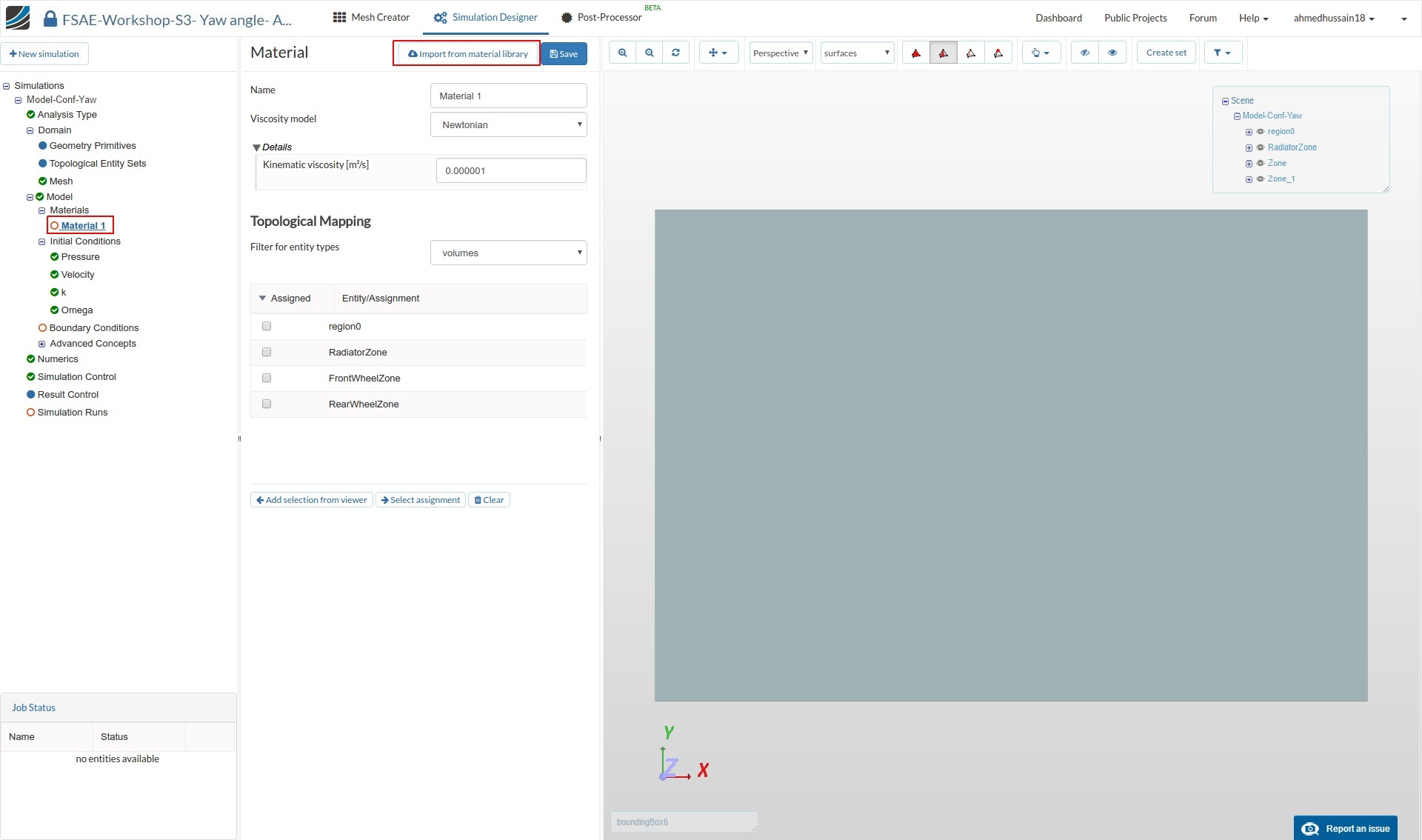
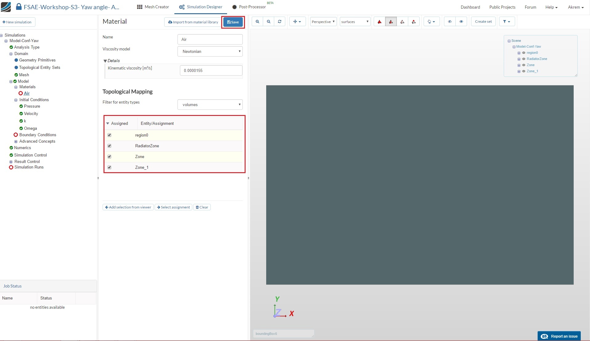
Select Air and click Save to import this material directly from the library.

Select region0, RadiatorZone,** Zone, and Zone_1 under Topological Mapping

Then click Save

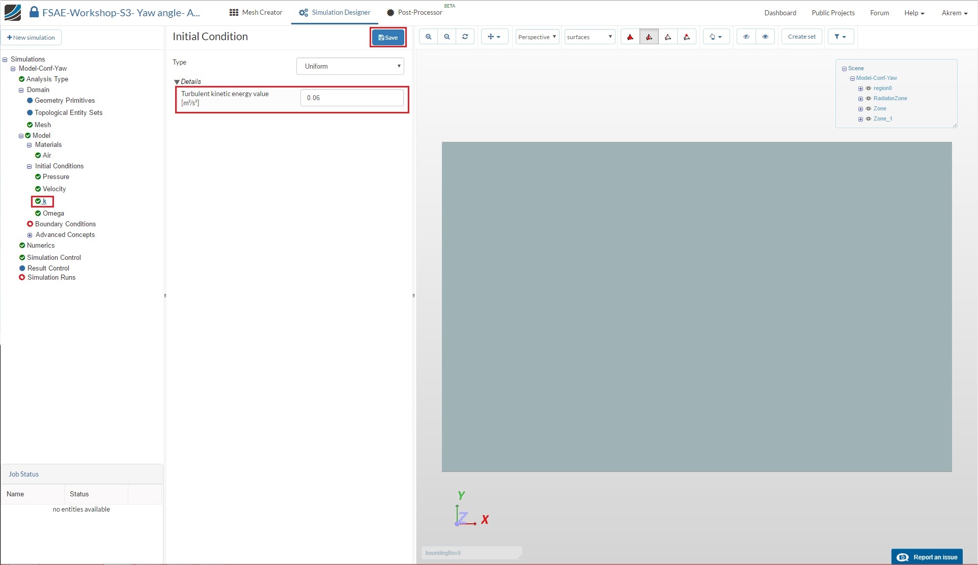
Initial Conditions

We will now proceed to change the initial conditions. Go to k and change the Turbulent kinetic energy value [m²/s²] value to 0.06 and click Save.

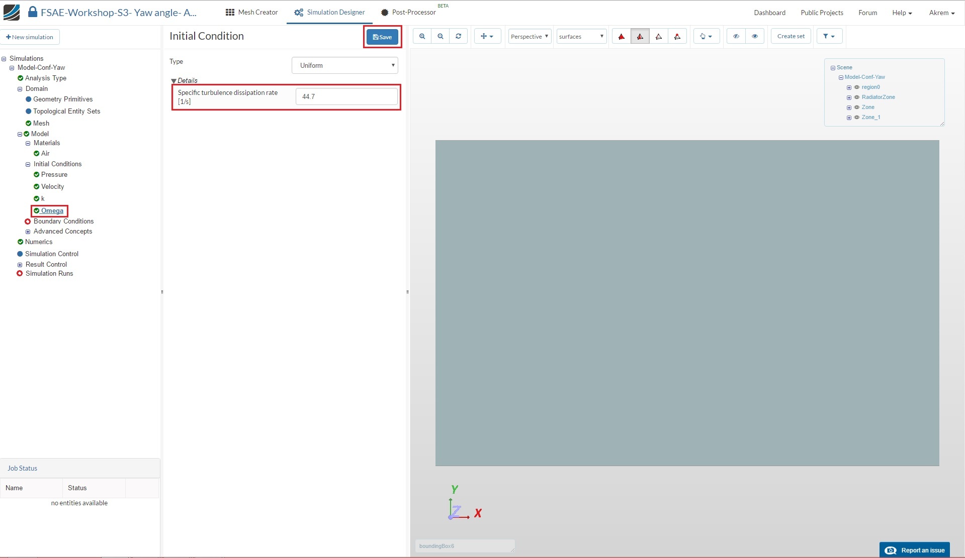
Next go to Omega and change Specific turbulence dissipation rate [1/s] to 44.7 and click Save.

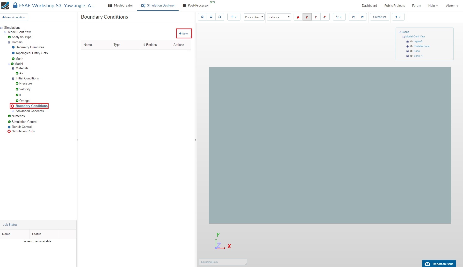
Boundary Conditions

Now we will proceed to the most crucial and important section of the simulation setup. We will define one by one the inlet boundary condition, and it will be different this time, because we want to investigate the side wind effect so we will customize the inlet boundary condition to control the angle of the free stream according to the car. We will then define the boundary condition for the sides, and next we will proceed to define the conditions for floor the roof and car, you have noticed that we don’t have symmetry plan like in the previous session because we are working with the full car.

Go to Boundary Conditions and click New in order to create a new boundary condition.

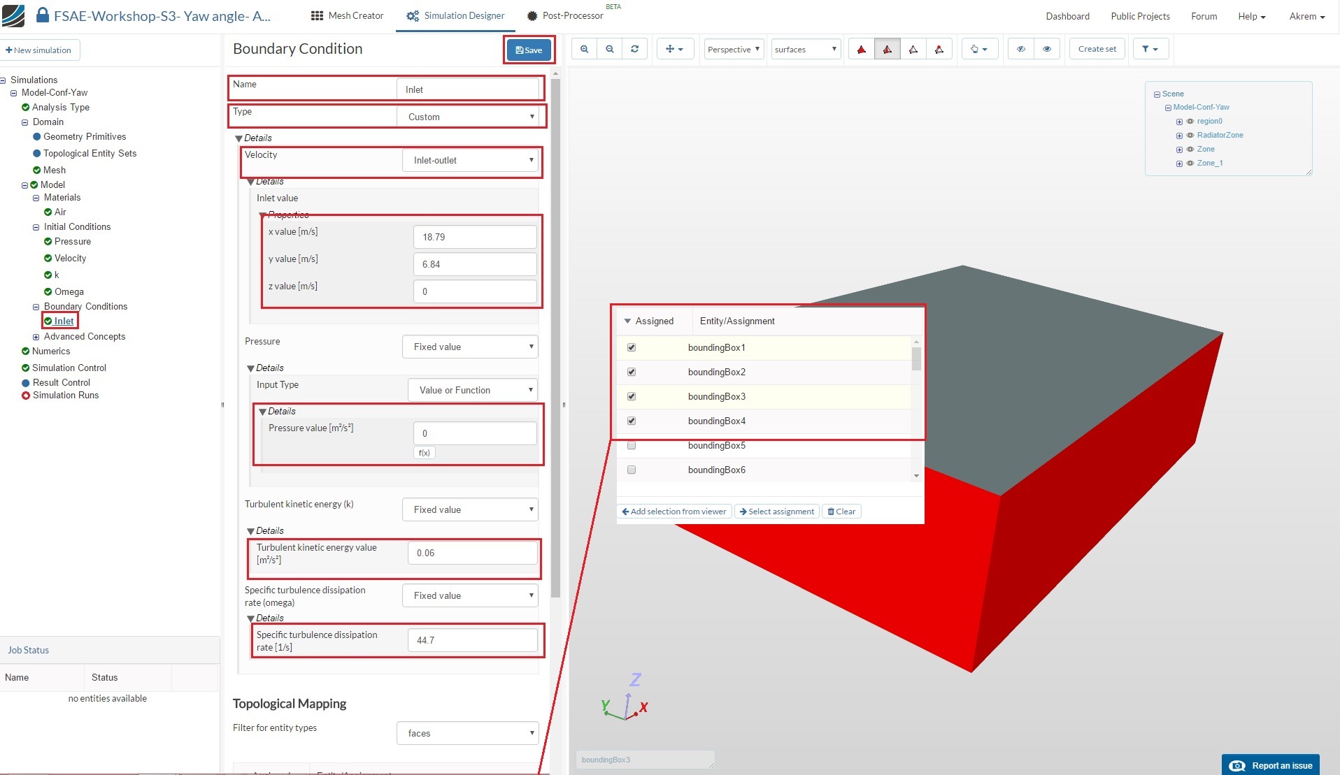
Inlet

Name the newly created boundary condition to Inlet (optional).

Set the Type to Custom

Under details select inlet outlet for velocity

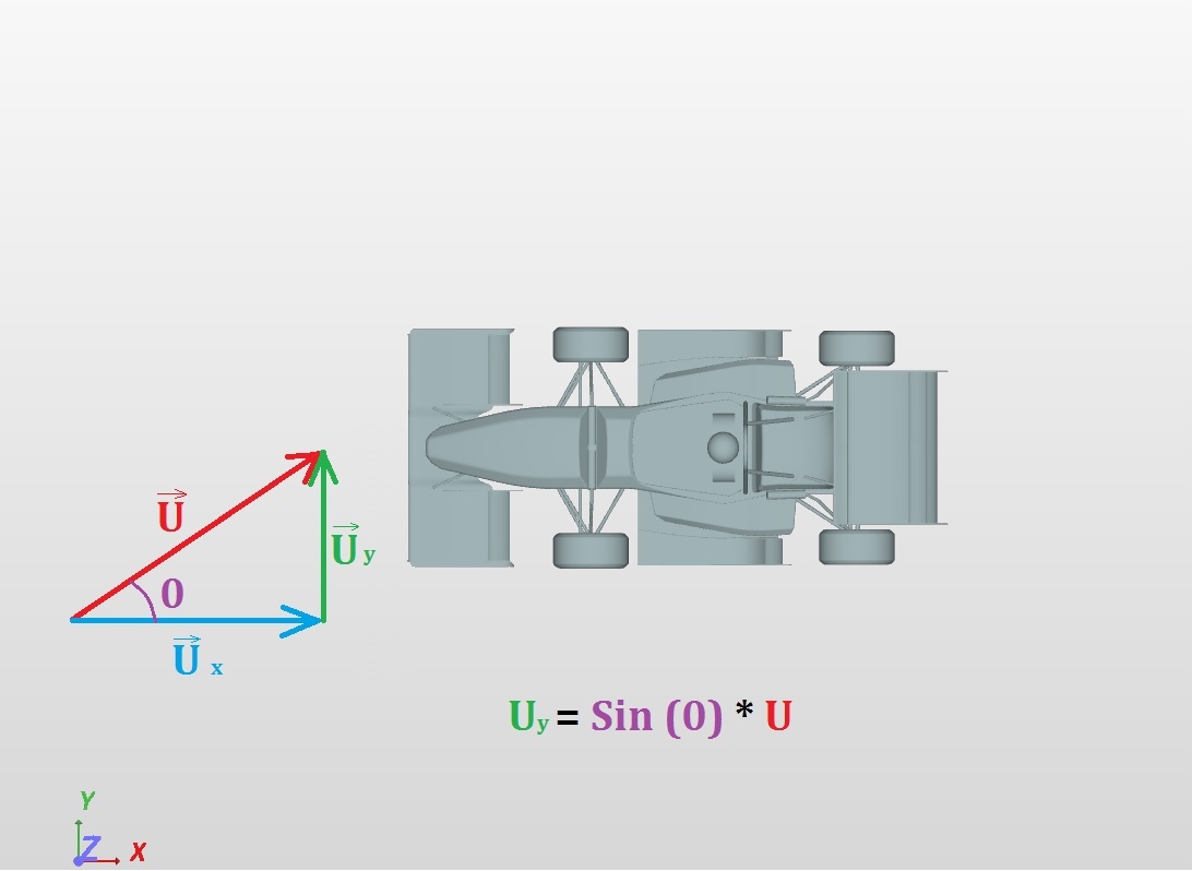
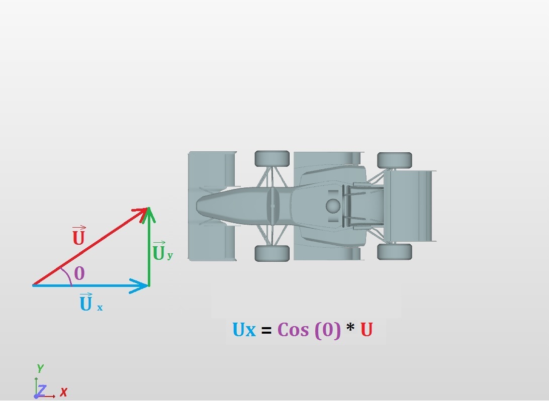
Then under details inlet valve > properties we will specify the X and Y components of the velocity vector depending on the freestream angle of 20°,

We calculate the velocity components with the help of trigonometric ratios formulas calculate the X component with Cos ratio and Y component with Sin ration (check the picture below), for 20° X value =18.79 [m/s] and Y value = 6.84 [m/s]

For Pressure select Fixed value and under Details > Details for pressure keep the value of 0[m²/s²]

For (K) Turbulent kinetic energy value [m²/s²] value and (Omega) Specific turbulence dissipation rate [1/s] respectively under details enter 0.06 and 44.7.

Assign the Topological Mapping to boundingBox1, boundingBox2, boundingBox3, boundingBox4 and click Select assignment in order to see the selected assignment in viewer.

Click Save

The formula to calculate Uy:

The formula to calculate Ux:

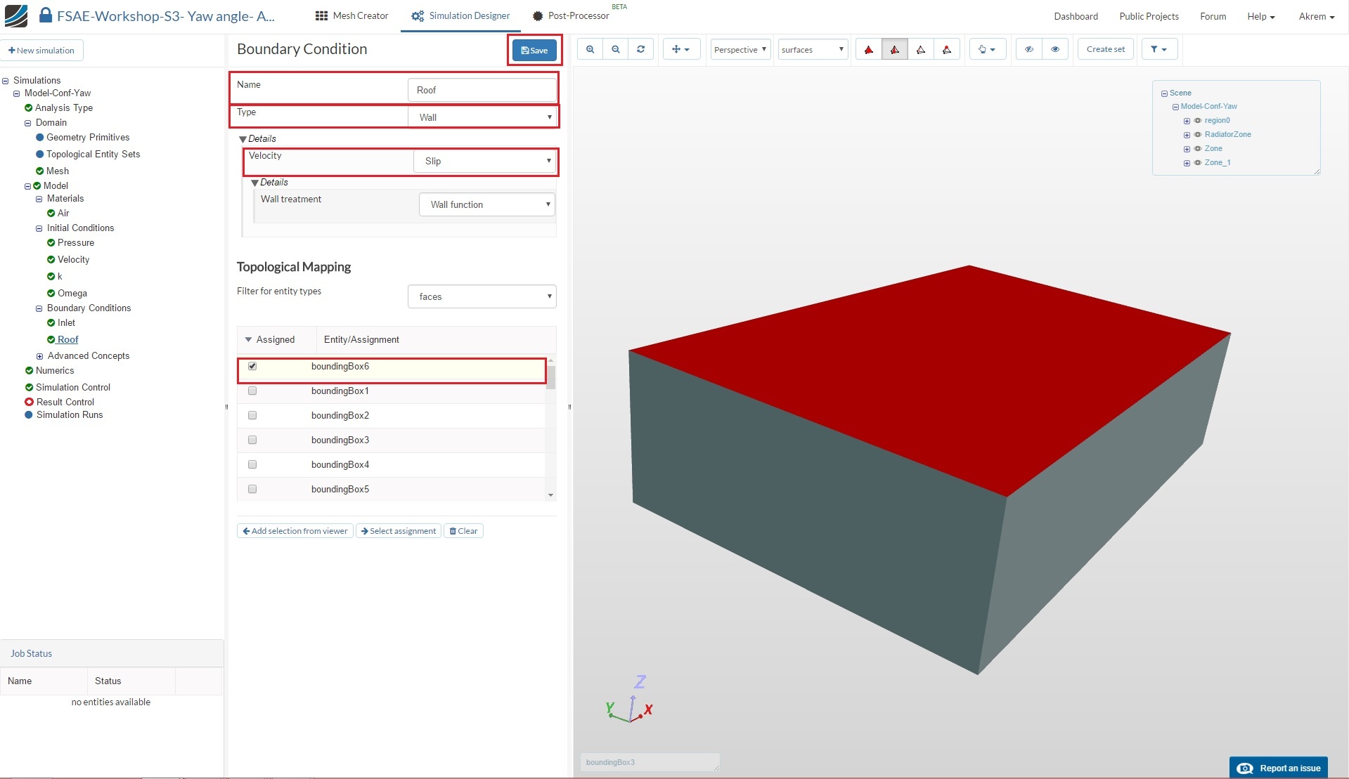
Roof

Create a new boundary condition named Roof (optional).

Change the Type to Wall and under details select Slip

Assign the boundary condition to boundingBox6 under Topological Mapping

Click Save

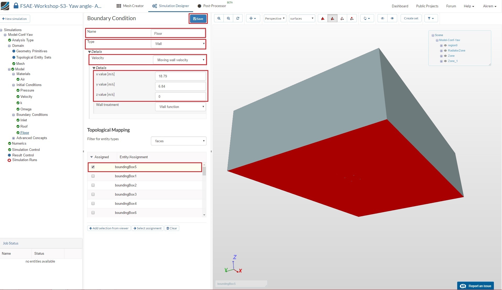
Floor

We will now define a moving floor boundary condition. Create a new boundary condition named Floor (optional).

Change the Type to Wall and under details set Velocity to Moving wall velocity. Because we are investigating side wind we have to enter the same vector components of the inlet velocity: x value [m/s] to 18.79and y value [m/s] to 6.84

Select boundingBox5 under Topological Mapping and click Select assignment in order to see the selected assignment in viewer. Click Save to define the floor boundary condition.

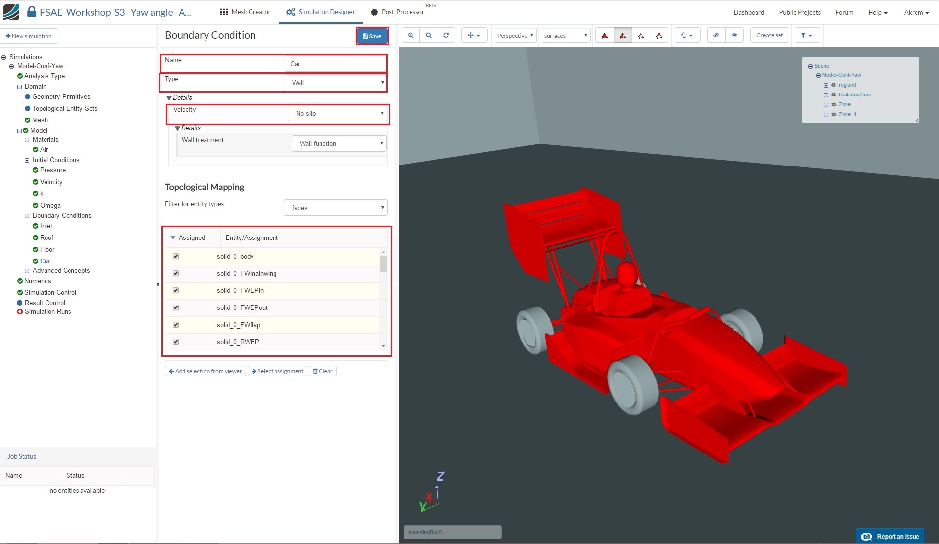
Car

Create a new boundary condition named Car (optional).

Change the Type to Wall and select all the entities starting with solid_0 except for solid_0_Reartire, solid_0_Fronttire

Click Save to define the boundary condition for the car.

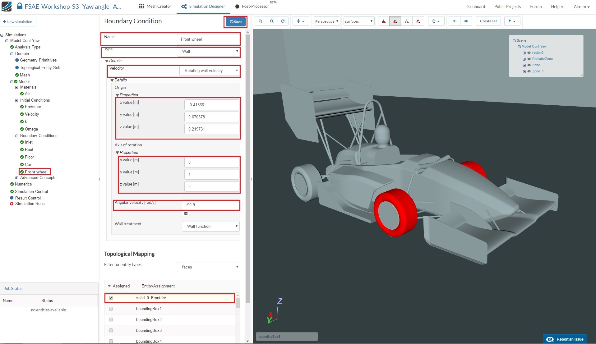
Front Wheel

Next we will add a rotating boundary condition for the wheels. Create a new boundary condition named Front wheel (optional).

Change Type to Wall and Velocity to Rotating wall velocity. Then change:

1. Origin x value [m], y value [m] and z value [m] value to -0.41566, 0.670378 and 0.219731 respectively.

2. Axis of rotation x value [m] and y value [m] to 0 and 1 respectively.

3. Angular velocity [rad/s] to -90.9

4. Then select solid_0_Fronttire under Topological Mapping and click Select assignment in order to see the selected item in the viewer.

5. Click Save to register your changes.

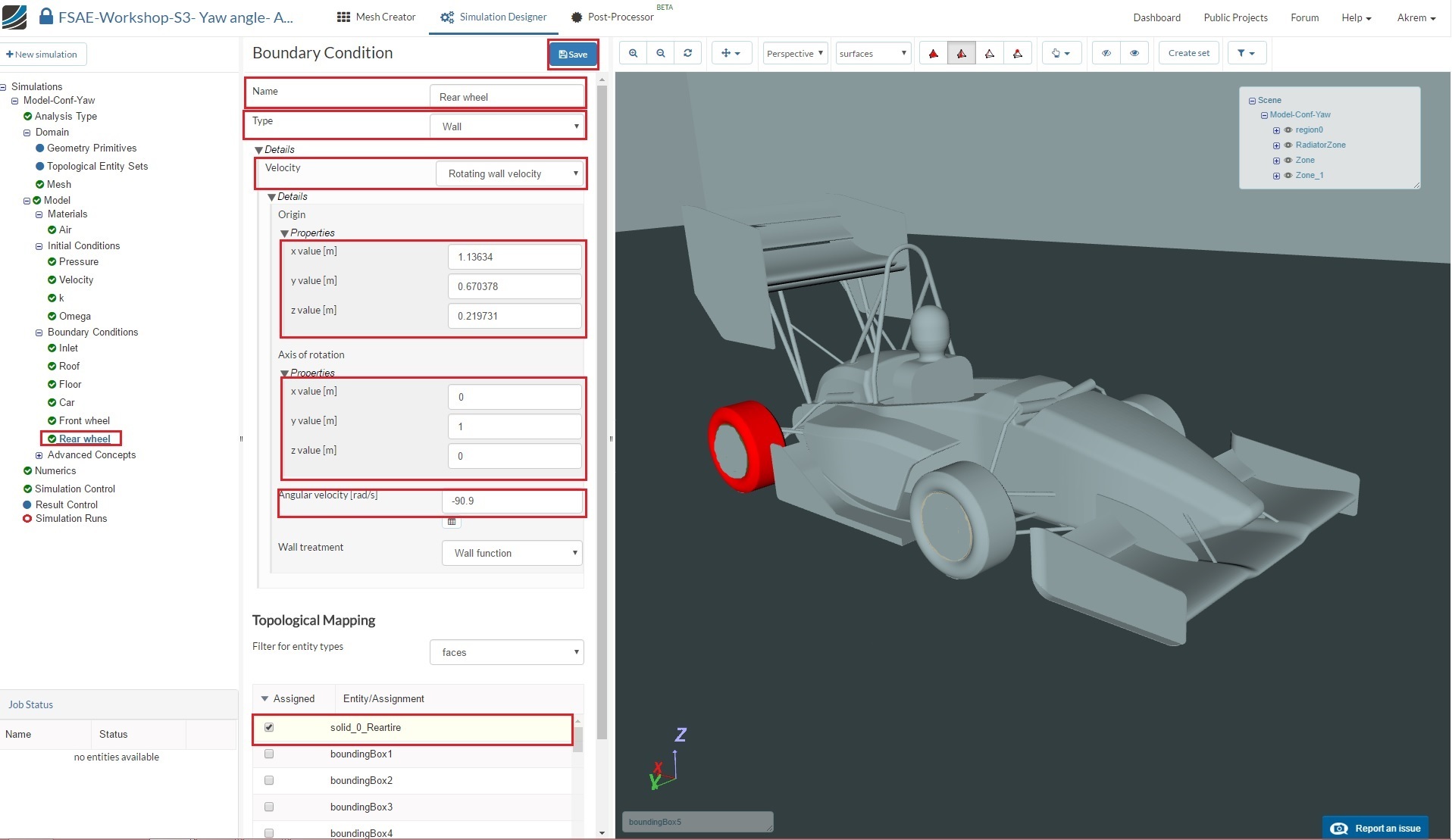
Rear Wheel

Create a new boundary condition named Rear wheel (optional). Change Type to Wall and Velocity to Rotating wall velocity. Then change:

1. Origin x value [m], y value [m] and z value [m] value to 1.13634, 0.670378 and 0.219731 respectively.

2. Axis of rotation x value [m] and y value [m] to 0 and 1 respectively.

3. Angular velocity [rad/s] to -90.9

4. Then select solid_0_Reartire under Topological Mapping

5. Click Save to register your changes.

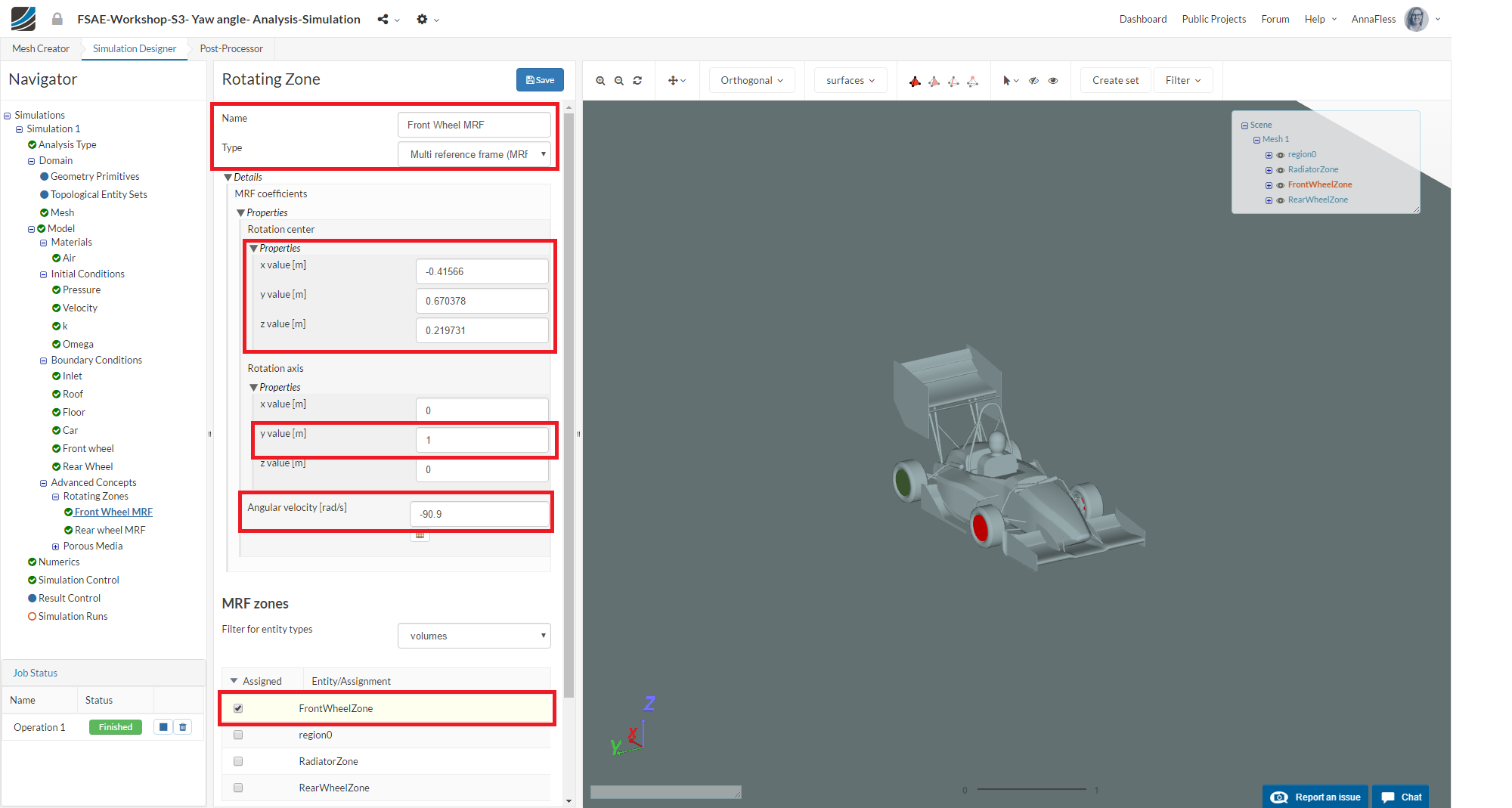
MRF zones

Add a Rotating Zones under Advanced Concepts named Front wheel MRF. Then change:

1. Origin x value [m], y value [m] and z value [m] value to -0.41566, 0.670378 and 0.219731 respectively.

2. Axis of rotation x value [m] and y value [m] to 0 and 1 respectively.

3. Angular velocity [rad/s] to -90.9

4. Then select FrontWheelZone under Topological Mapping

5. Click Save to register your changes.

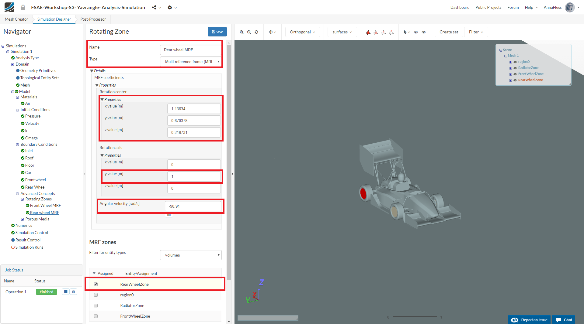
Similarly, perform the same procedure and create a new Rotating Zone. Rename it to Rear wheel MRF. Then change:

1. Rotation center x value [m], y value [m] and z value [m] value to 1.13634, 0.670378 and 0.219731 respectively.

2. Rotation axis y value [m] to 1

3. Angular velocity [rad/s] to -90.91

4. Then select RearWheelZone under MRF zones and click Select assignment in order to see the selected item in the viewer.

5. Click Save to register your changes.

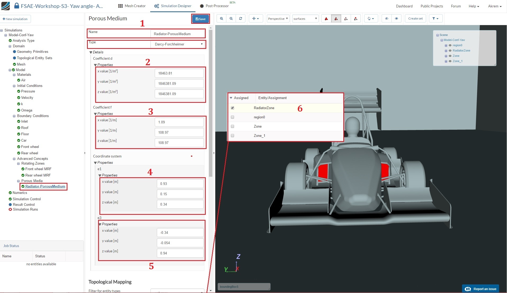
Porous Media

In this section we will define the radiator volume source via porous media. Expand the Advanced Concepts tree item and proceed to Porous Media. Click +New to create a new porous media definition.

After creating a new porous media definition, you will be automatically directed to the properties panel. Change:

1. Name to Radiator-PorousMedium (optional).

2. Coefficient d x, y and z values to 18463.81, 1846381.09 and 1846381.09 respectively.

3. Coefficient f x, y and z values to 1.09, 108.97 and 108.97 respectively.

4. Coordinate system e1 x, y and z values to 0.93, 0.15 and 0.34 respectively.

5. Coordinate system e3 x, y and z values to -0.34, -0.054 and 0.94 respectively.

6. Scroll down and select RadiatorZone under Topological Mapping.

7. Click Select assignment to see the selected volume source in viewer.

8. Click Save to register your changes.

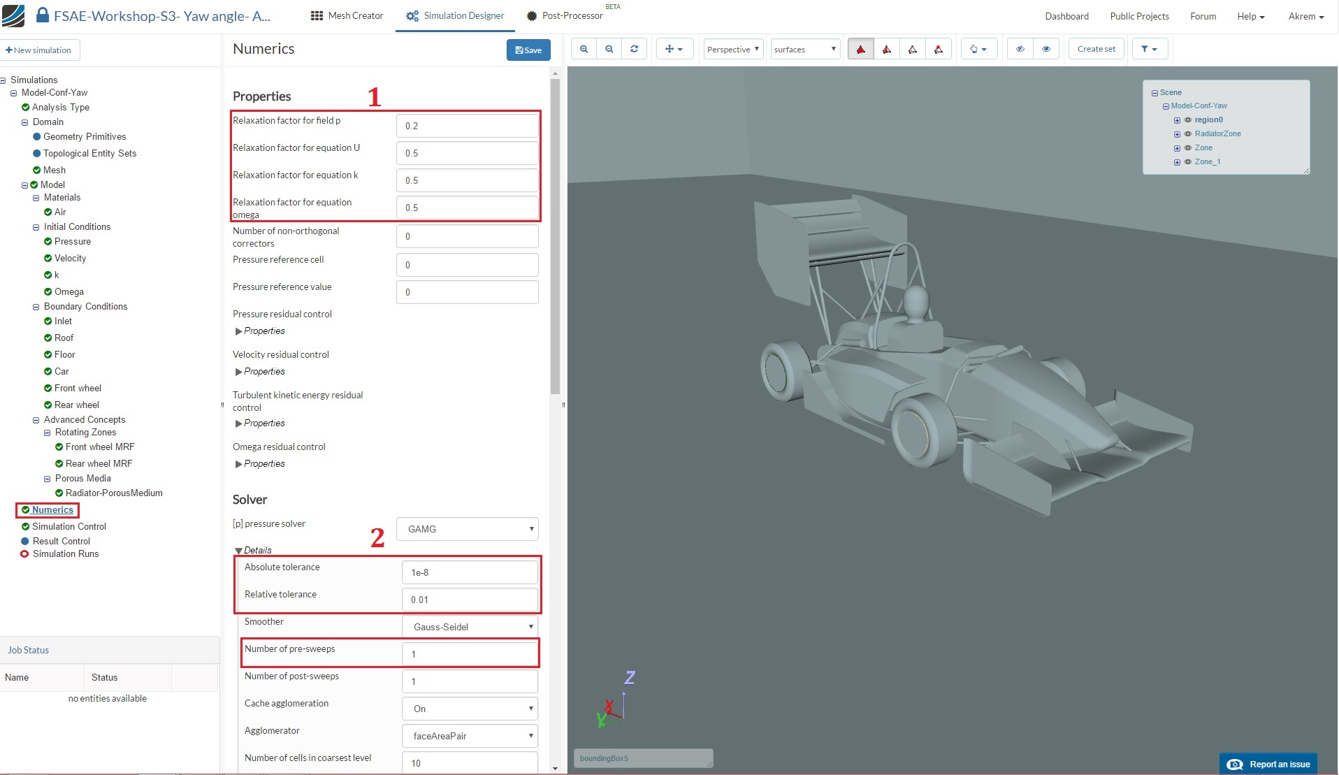
Numerics

After defining all the boundary conditions, we will proceed to set up the numerics for our simulation. Go to Numerics and change:

1. Relaxation factor for field p, Relaxation factor for equation U, Relaxation factor for equation k and Relaxation factor for equation omega to 0.2, 0.5, 0.5 and 0.5 respectively.

2. Furthermore, under [p] pressure solver, change Absolute tolerance, Relative tolerance and Number of pre-sweeps to 1e-8, 0.01 and 1 respectively.

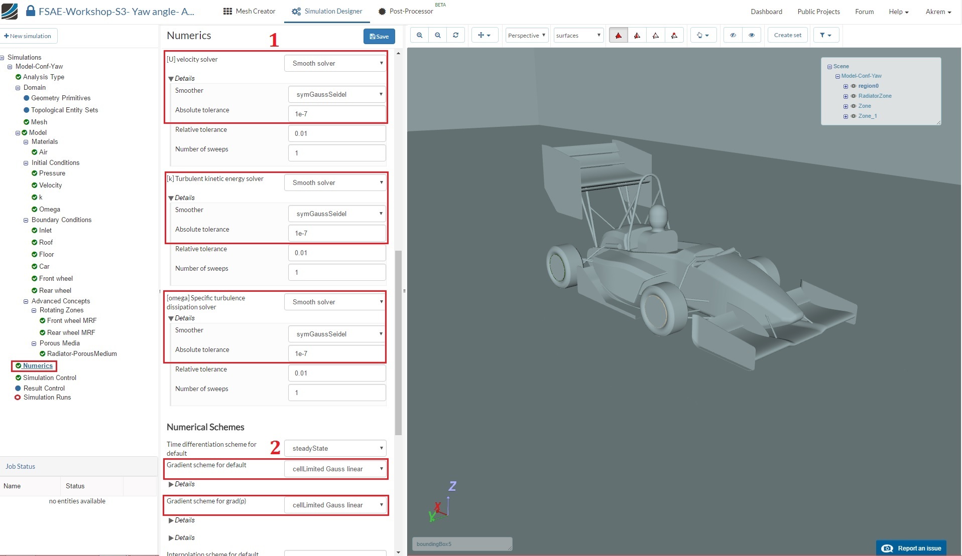
Scroll down until [U] velocity solver and change:

1. [U] velocity solver to Smooth solver, Smoother to symGaussSeidel and Absolute tolerance to 1e-7. Do the same for [k] Turbulent kinetic energy solver and [omega] Specific turbulence dissipation solver

2. BothGradient scheme for default and Gradient scheme for grad(p) to cellLimited Gauss linear

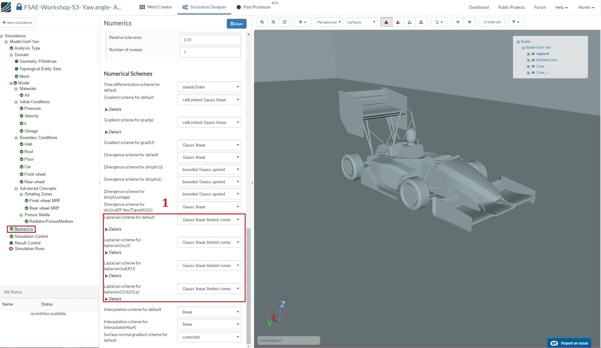
Scroll down to the end and change:

1. Laplacian scheme for default, Laplacian scheme for laplacian(nu,U), Laplacian scheme for laplacian(nuEff,U) and Laplacian scheme for laplacian((1|A(U)),p) to Gauss linear limited corrected

2. Click Save to register all of your changes.

For for more steps, please go to the following forum post: [Step-by-Step Tutorial: Homework of Session 3 section 2 - Further Setups and Post-processing]
(Step-by-Step Tutorial: Homework of Session 3 section 2)

[PNtakos]

I seem to be unable to import the project, I receive an error and get redirected to the dashboard. Is this only on my end?

[Akrem]

Hey @PNtakos fixed, try to open it mow .

[clav]

Can someone explain what the difference is between “mesh to geom conformatn iteratns” and “max iteratns for mesh confirmatn”? Shouldn’t the latter value be higher than the former?

[SebastianMJ]

Above the second to last picture before “Simulation Setup” it say

@Akrem

While the mesh is being generated, you can start setting up the mesh for the other geometry following the same procedure (Follow the details below).

I am not quite sure which other geometries are being spoken about since the remaining of the guide is in the simulation designer. Could anyone help me understand what other geometry are supposed to be meshed?

Thanks in advance,
Sebastian Jørgensen

[Akrem]

@SebastianMJ sorry for the mistake there is only one geometry in this home work.

[PNtakos]

I started the meshing process and I receive the “illegal triangles” error just like homework #2. Is there any confirmed reason why some of us get this message and others don’t?

Thanks in advance.

[AMartinezCava]

Got a memory error during the meshing process:

Checking faces in error :
non-orthogonality > 75 degrees : 0
faces with face pyramid volume < 1e-13 : 0
faces with concavity > 80 degrees : 0
faces with skewness > 4 (internal) or 20 (boundary) : 0
faces with interpolation weights (0…1) < 0.01 : 0
faces with volume ratio of neighbour cells < 0.0075 : 0
faces with face twist < 0.005 : 0
faces on cells with determinant < 0.001 : 0
Doing final balancing
---------------------
Found 147406 zoned faces to keep together.
Found 0 separated coupled faces to keep together.
(4): (9): ERROR: dgraphFold2: out of memory (2)
(12): ERROR: dgraphFold2: out of memory (2)
(1): ERROR: dgraphFold2: out of memory (2)
ERROR: dgraphFold2: out of memory (2)
-------------------------------------------------------
Primary job terminated normally, but 1 process returned
a non-zero exit code… Per user-direction, the job has been aborted.
-------------------------------------------------------
[11] #0 Foam::error::printStack(Foam::Ostream&)--------------------------------------------------------------------------
mpirun detected that one or more processes exited with non-zero status, thus causing
the job to be terminated. The first process to do so was:
Process name: [[257,1],4]
Exit code: 1

Any clues? Thanks in advance.

[igomez_r]

the last time i has that problem, it is a snappyHexMesh or parallel processing glitch, try using a different number of cores like 8.

[AMartinezCava]

@igomez_r

the last time i has that problem, it is a snappyHexMesh or parallel processing glitch, try using a different number of cores like 8.

Thanks, will give it a try. But if it runs out of memory with 32 cores, I don’t know if it will mange to complete it using 16…

[jousefm]

@AMartinezCava,

if you have problems with the mesh or you are afraid that you might use a lot of your core hours for this process, I can do the meshing job for you if you like.

Cheers!

[amaknojia]

After Finishing Meshing, found illegal cells:

non-orthogonality > 75 degrees : 59
faces with face pyramid volume < 1e-13 : 2
faces with concavity > 80 degrees : 0
faces with skewness > 4 (internal) or 20 (boundary) : 0
faces with interpolation weights (0…1) < 0.01 : 0
faces with volume ratio of neighbour cells < 0.0075 : 7
faces with face twist < 0.005 : 44
faces on cells with determinant < 0.005 : 33
Finished meshing with 145 illegal faces (concave, zero area or negative cell pyramid volume)

–>Is it safe to continue to simulation phase?

Also, there are no settings outlined for the simulation run.

[DeorajA]

@Milad_Mafi @Akrem Please answer.
Even I finished with 141 illegal faces.

[adewade]

sir my geometry file is not importing.It will be deleted by myself when i opened it for first time.give me suggestion

[s_giuliano]

hi…please anyone could help me??? i have some problems in launching simulation after doing the mesh…before the launch, i check errors but the software can’t find them…this is my project https://www.simscale.com/workbench?publiclink=7ecb9e14-b234-48e6-8359-461a540c1070 thank you …

[s_giuliano]

after 30 minutes the simulation ends and the software tells me "ERROR "

[Milad_Mafi]

Hey,

@PNtakos

started the meshing process and I receive the “illegal triangles” error just like homework #2. Is there any confirmed reason why some of us get this message and others don’t?

Thanks in advance.

Everyone is receiving the message. It is related to the triangles of the geometry, which was uploaded using the STL file format. In contrast to CAD file formats like STEP or IGES, STL represents the geometry with small triangles instead of using infinite precise spline functions.

The error warning basically sets that there is a an issue with the STL file. This is most of the times related to numerical problems and therefore you should not get confused by this message.

Cheers,

Milad

[Milad_Mafi]

@DeorajA @amaknojia

Sometimes you can not avoid illegal cells. This error message only tell you the number of cells which are not fulfulling certain quality criteria. But it doesn’t tell you how bad the quality actually is. You can have 1 or 2 cells that are really bad can affect your simulation and maybe you have 100 but not so much just under the control value and you will get right results.

I followed the instructions step-by-step an I got 96 illegal cells in total.

---------------------
Layer mesh : cells:12088700 faces:39430079 points:15496971
Cells per refinement level:
0	205190
1	8342
2	55644
3	44252
4	198318
5	1072718
6	2548783
7	3236275
8	4719178
Writing mesh to time constant
Wrote mesh in = 32.52 s.
Layers added in = 394.54 s.
Checking final mesh ...
Checking faces in error :
non-orthogonality > 75 degrees : 3
faces with face pyramid volume < 1e-15 : 1
faces with concavity > 80 degrees : 27
faces with skewness > 4 (internal) or 20 (boundary) : 2
faces with interpolation weights (0..1) < 0.01 : 0
faces with volume ratio of neighbour cells < 0.0075 : 4
faces with face twist < 0.005 : 35
faces on cells with determinant < 0.005 : 24
Finished meshing with 96 illegal faces (concave, zero area or negative cell pyramid volume)
Finished meshing in = 1273.26 s.
End
Finalising parallel run

Cheers,

Milad