NOTE: This tutorial was updated on 08/2016 to match the updated version of the platform
If you would like to watch the second session of the Drone Workshop again or in the case you missed it, you can access the full recording below.
 - Static Structural Simulation of a Drone Part")
Level 2
Preface
Since our drone consists of different components from different materials, they have to be connected somehow. In this case we are manly using screws to connect these parts. One of the most loaded connection is the one between the drone arm and the two base plates.
The decisive factor for the stability of this connection is the preload between the base plates and the arm which can be controlled by the tightening of the nut. The simplification we made in the first level of this homework can therefore have a big impact on the deformation of the arm.
Exercises
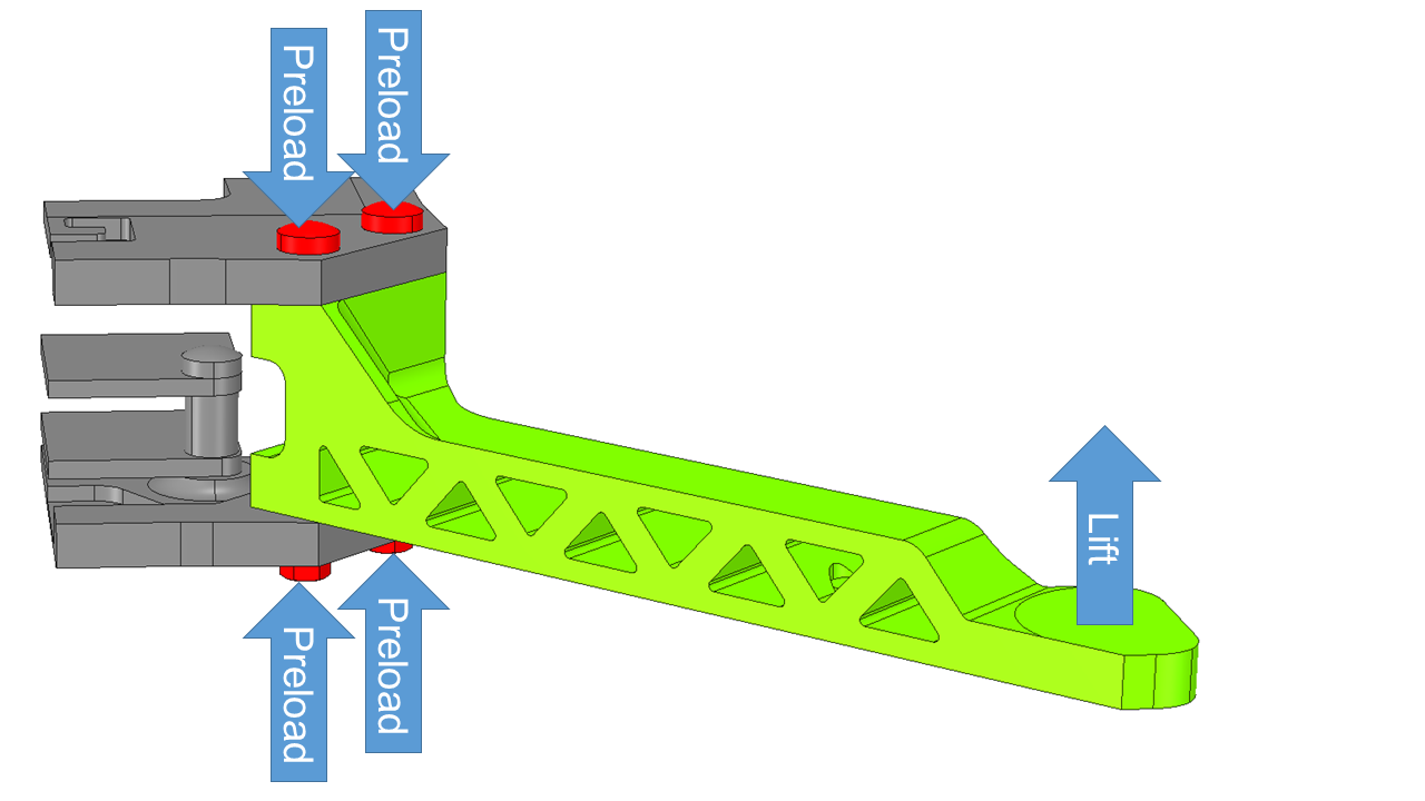
Our aim is to set up the deformation of the drone arm when applying the lift force on it. In contrast to the level 1 exercise where we just fixed two sides of the arm, in this level we will use the full assembly of the drone arm including the screw connection to consider the preload of the screws and the connection between arm and base plates.
Additonaly to this we will investiage the effect of mesh refinement on the result. We will therefore perform the simulation with a coarse and a fine mesh.
Step-by-Step instruction
Note: These instructions refer to the coarser mesh. For the finer mesh just replace the refinement parameters for both mesh refinements by the values which you find at the end of this tutorial.
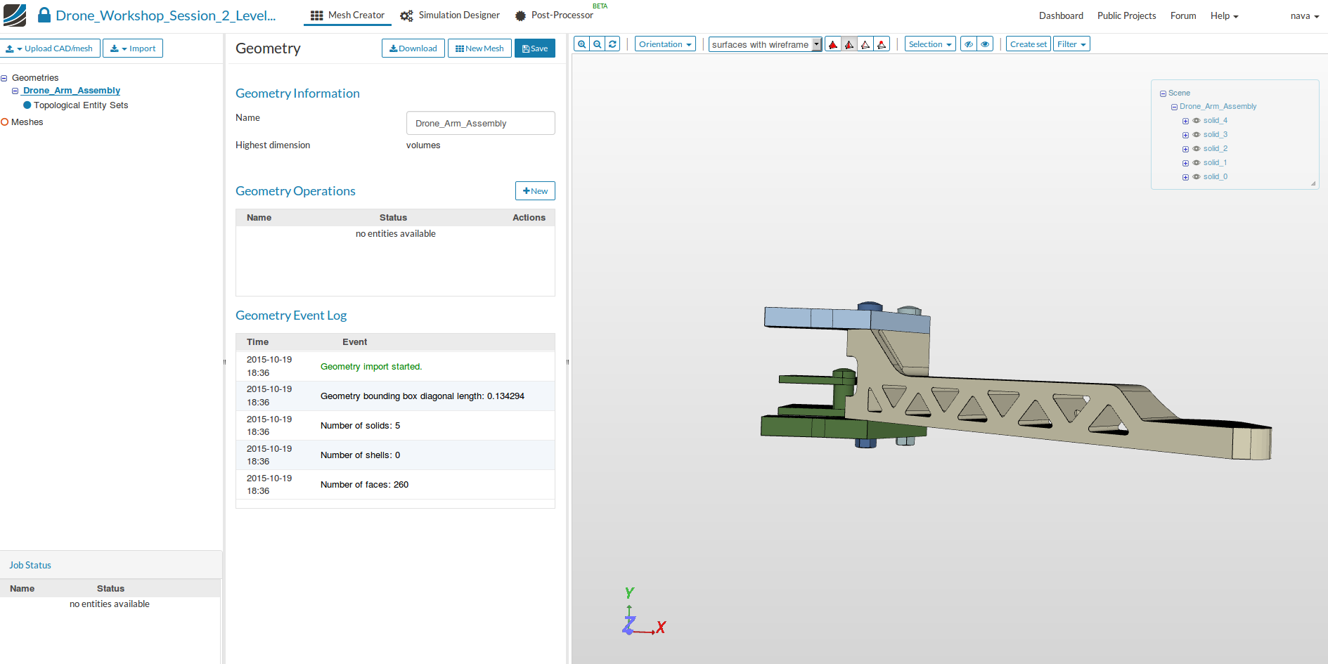
First of all you have to import the geometries into your SimScale workspace. For this, you only have to click on this link and a project with everything you need will be added to your workspace. Please note that this can take several minutes.
Meshing
- In the Mesh Creator tab, click on the geometry Drone_Arm_Assembly
- Then, click on New Mesh button in the options panel.
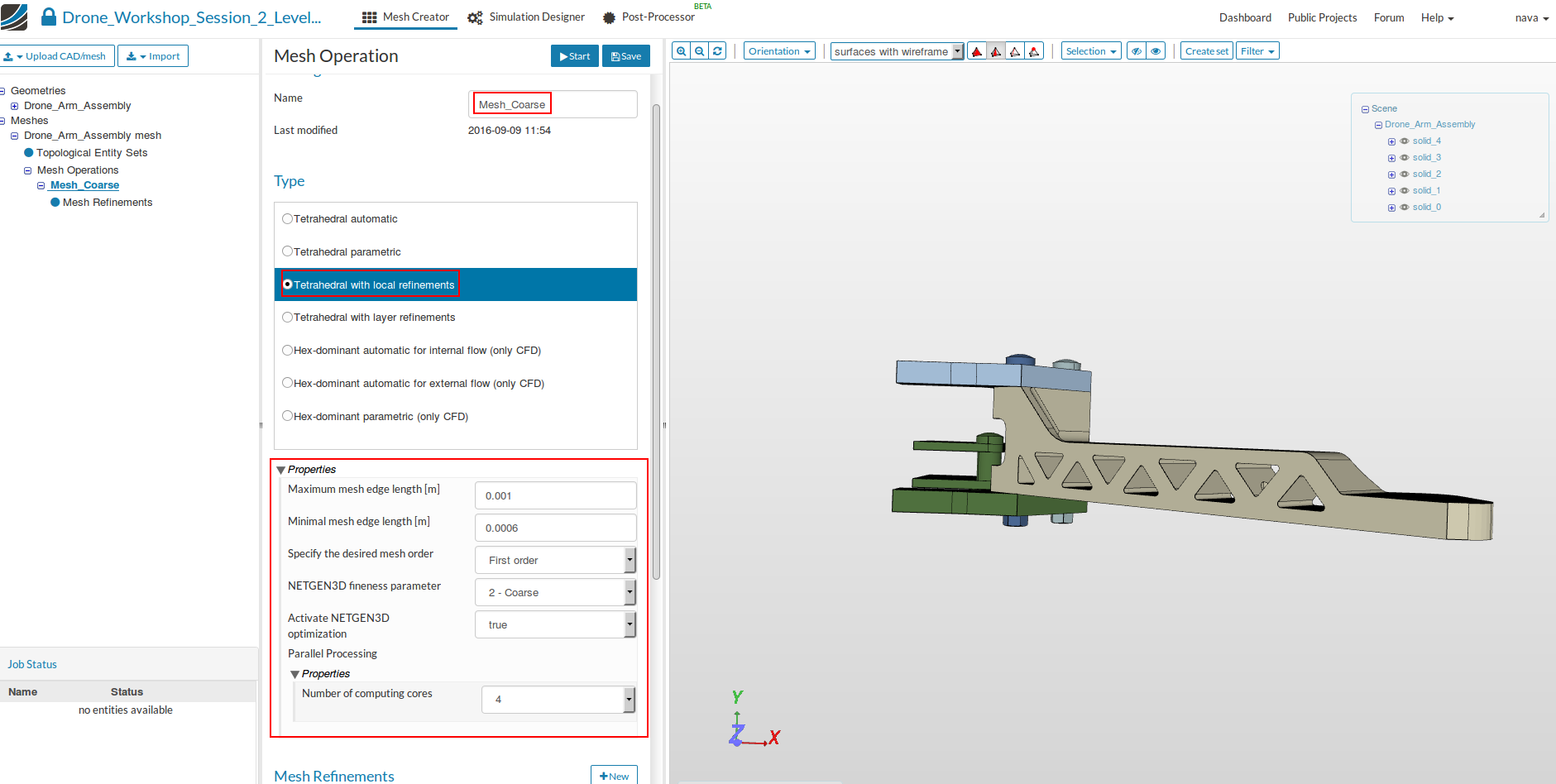
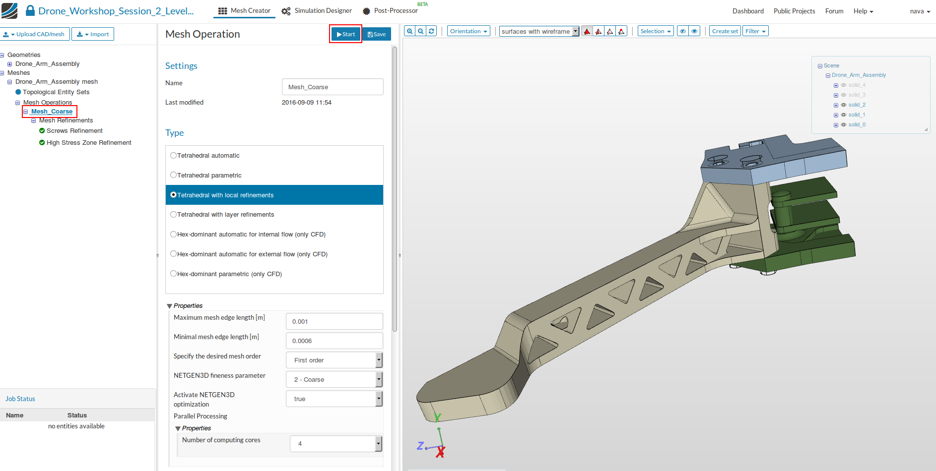
- Select Tetrahedral with local refinements and define following parameters:
- Name: Mesh_Coarse (optional)
- Maximum mesh edge length [m]: 0.001
- Minimal mesh edge length [m]: 0.0006
- Specify the mesh order: First order
- NETGEN3D fineness parameter: 2 - Coarse
- Activate NETGEN3D optimization: true
- Number of computing cores: 4
- Click on Save to save the setting.
Now we have defined a range for the base mesh size which is fine for regions where we are not expecting high stress. Here you should keep in mind that, in general, the mesh size is related to the local accuracy of the simulation. It is therefore necessary to refine the mesh in those areas where high stresses is expected and the curved surfaces with very small curvatures (fillets) where the stress concentration will appear.
We will now apply local refinements on two areas where we expect high stresses and high deformations.
We will start with the two screws which connect the arm with the two base plates.
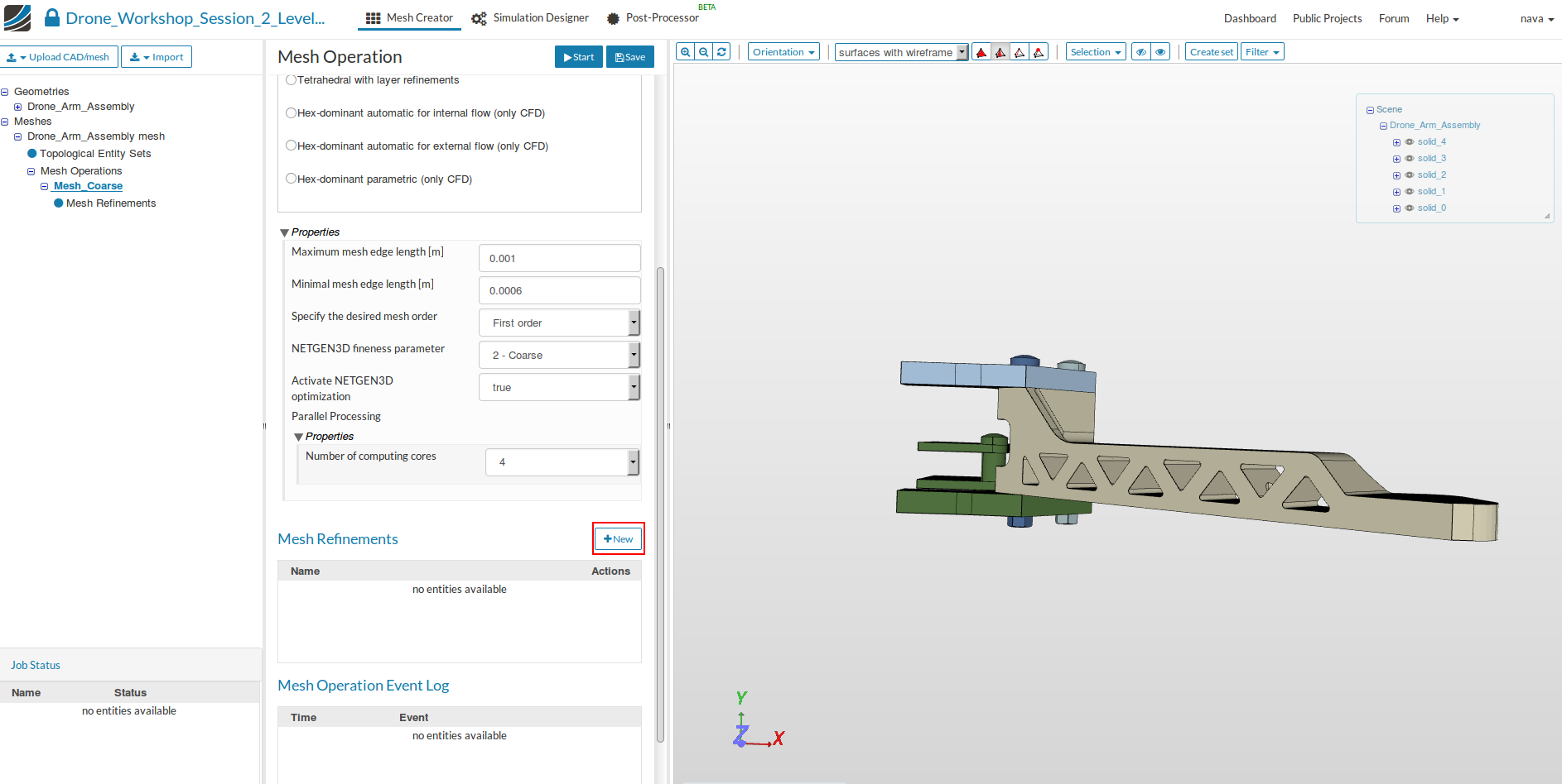
- Click on the New button under Mesh Refinement.
- Specify the following parameters
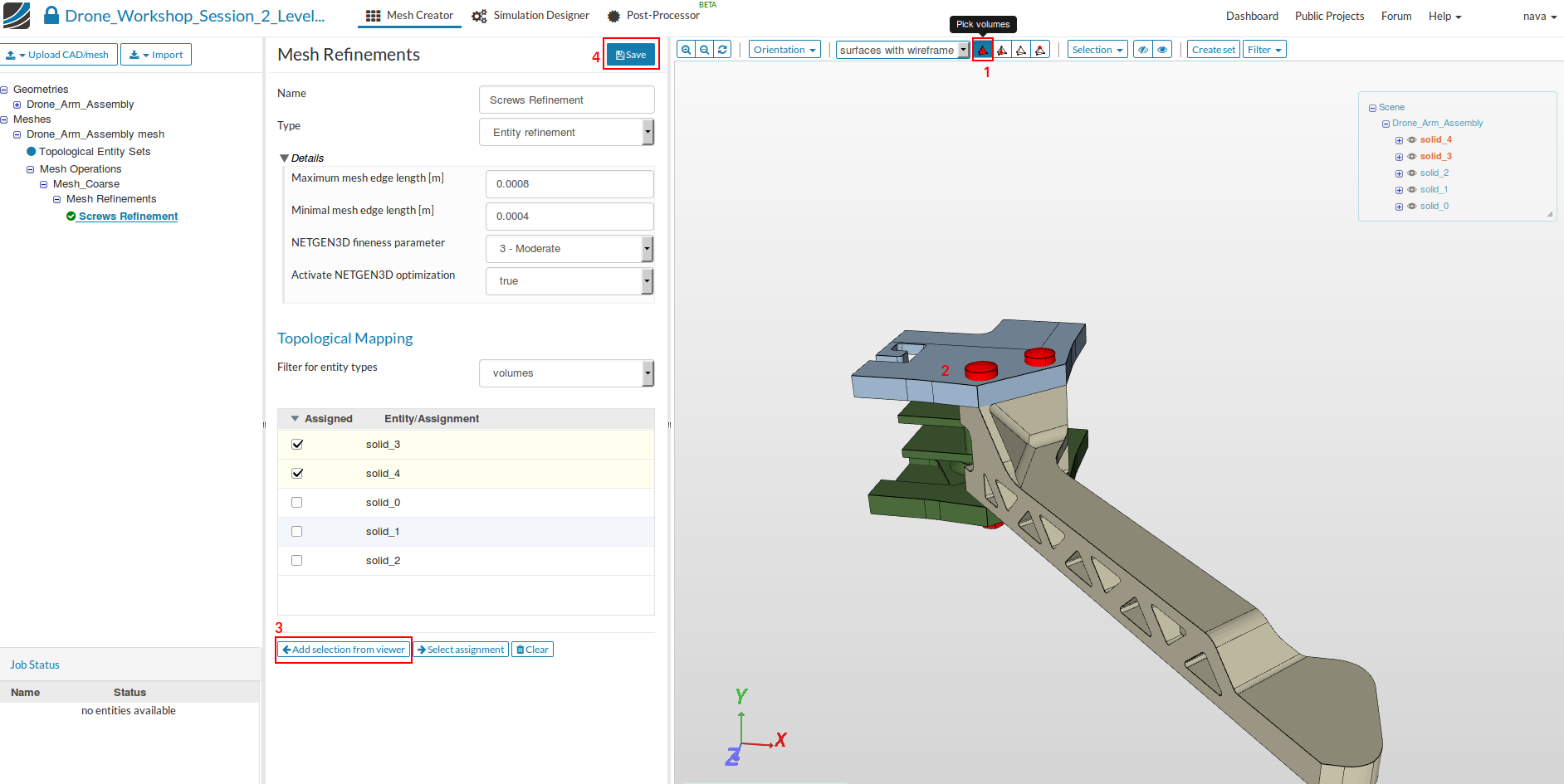
- Name: Screws Refinement (optional)
- Maximum mesh edge length: 0.0008
- Minimal mesh edge length: 0.0004
- NETGEN3D fineness parameter: 3 - Moderate
Now we have to assign the volume where we want apply this mesh refinement.
- Change the selection mode to volume (1) select the volumes in the 3D model window on the left side by clicking on them with the left mouse button (2) ; to add them to the list, just click on the Add selection from Viewer button in the middle column (3) and Save your settings (4).
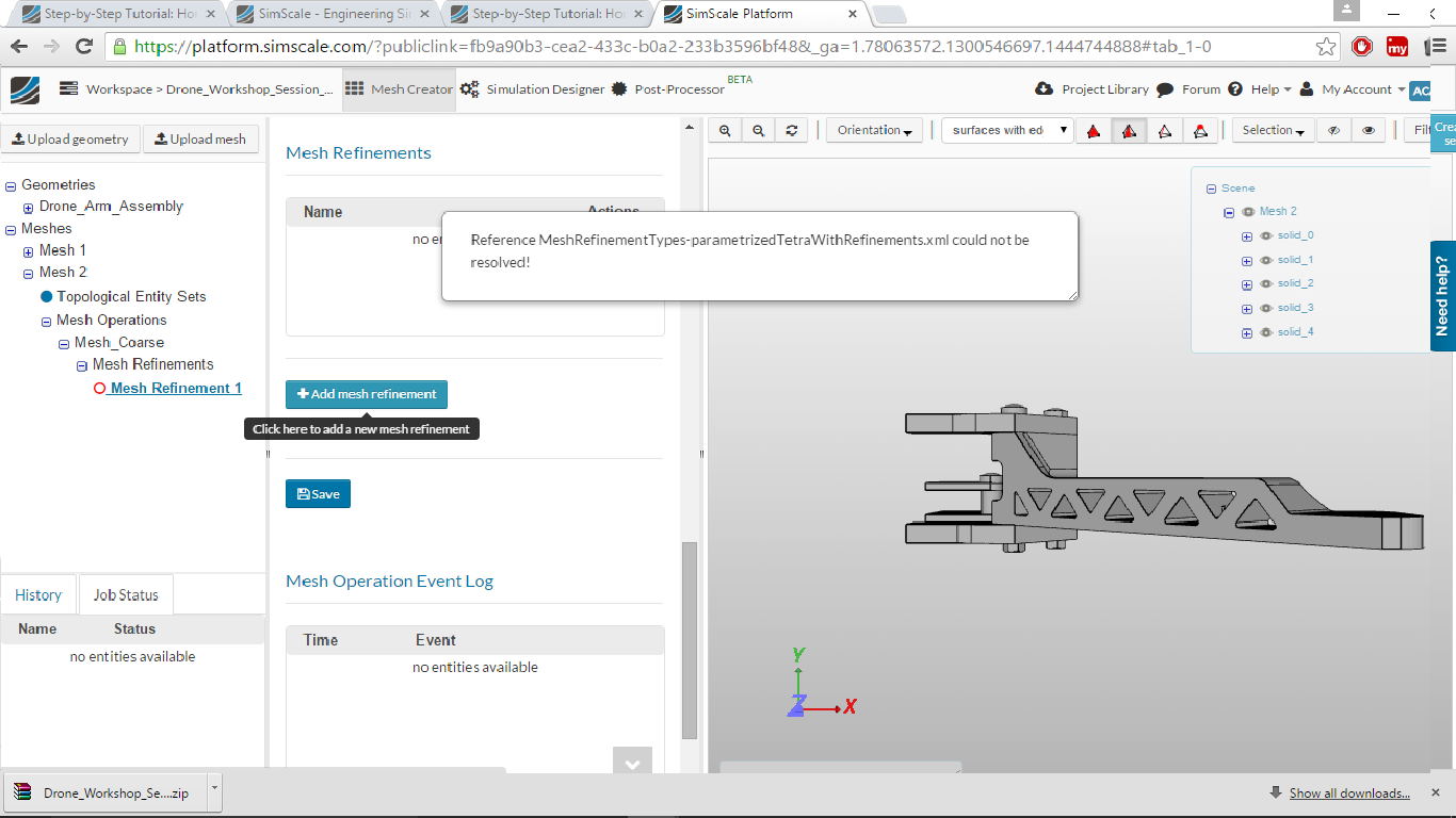
- Create an additional mesh refinement by clicking on the Mesh refinements in the project tree and then Click on New button.

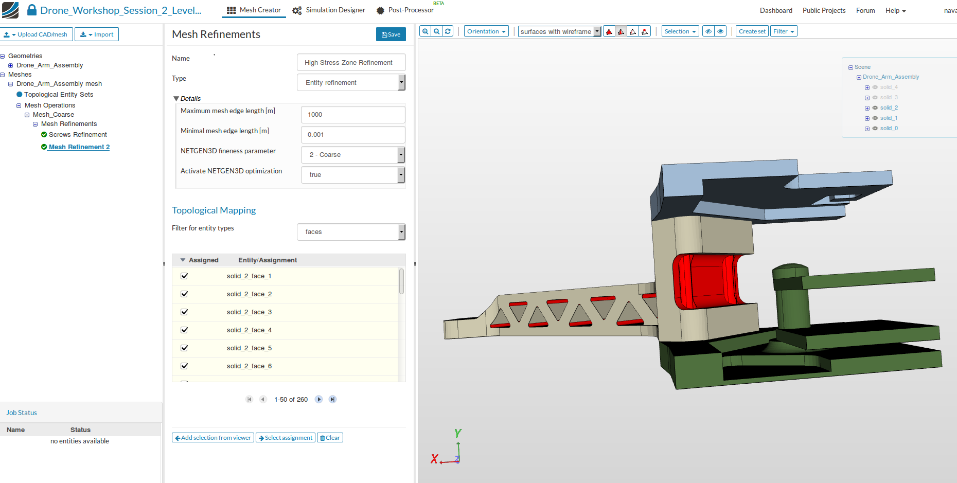
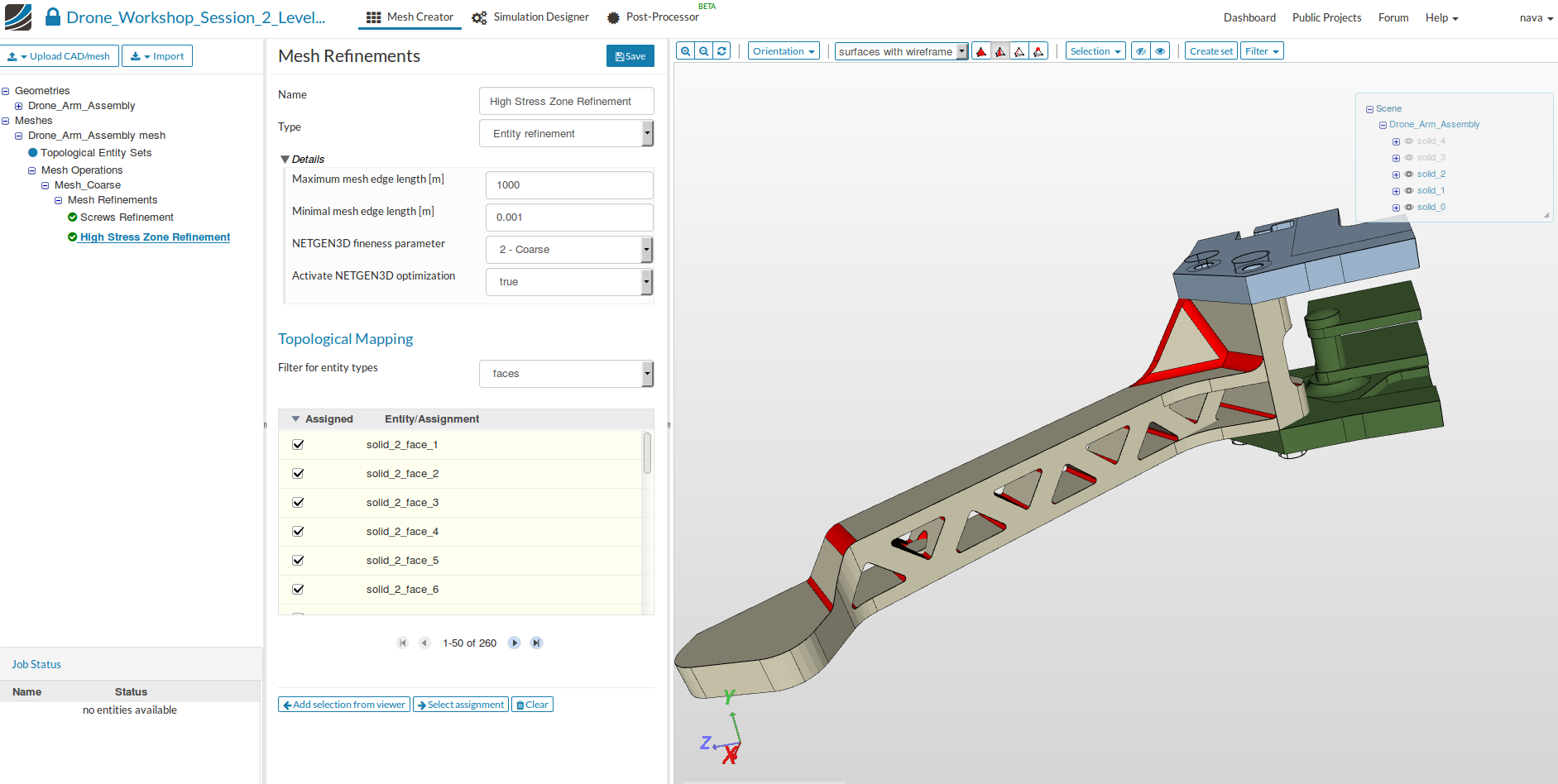
- Now we will add refinement to some curved surfaces of the arms and the base plates. Specify the refinement as follows:
- Name: High Stress Zone Refinement (optional)
- Maximum mesh edge length: 0.0003
- Minimal mesh edge length: 0.0001
- NETGEN3D fineness parameter: 3 - Moderate
-
Choose faces for Filter for entity types and click on
 so that you can select the faces which you need to refine. For this, click on the eye symbol in the model tree to hide them (solid 3 and solid 4).
 -
Select all the faces shown in the figure below and click on Add selection from viewer to assign the mesh refinement to all the curved surface and Save the settings.
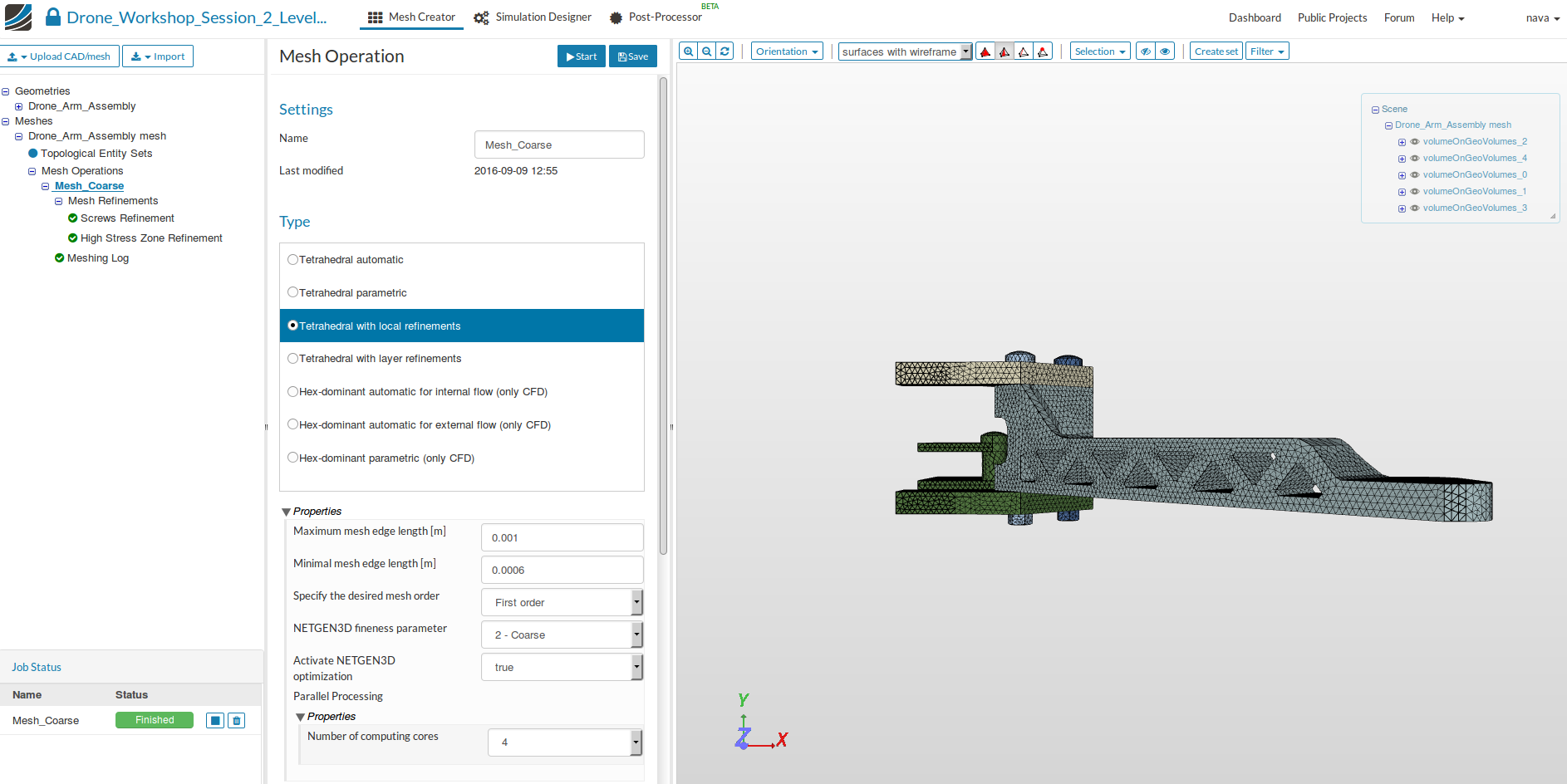
- Now our mesh is ready for computation. Click on the Coarse_mesh in the project tree and click the Start button.
- Once the mesh computation is finished, you will see Finished status in lower left corner and in the viewer you will see the meshed geometry.
Simulation Setup
-
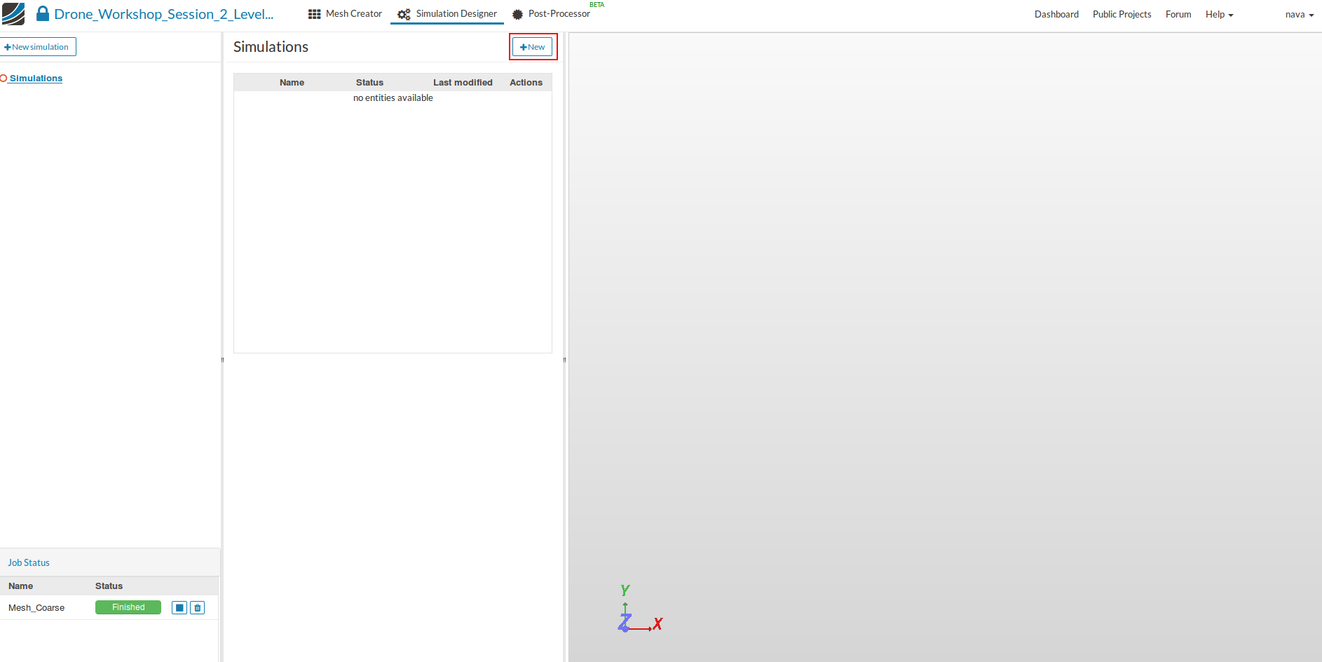
After the mesh is completed we will set up the simulation. Click on the Simulation Designer tab.
-
Click on New button to create a new simulation and give it a suitable name- Mesh_Coarse (optional).
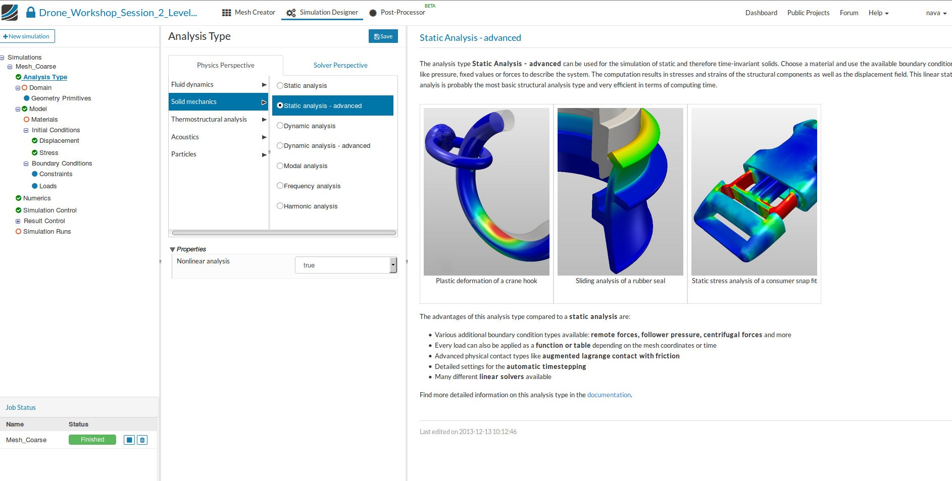
- Select Static analysis - advanced as Analysis Types, set Nonlinear analysis to True and then click on Save.
Going forward, this tree will guide us through all necessary steps. Please note that some of the items are optional.
Domain selection
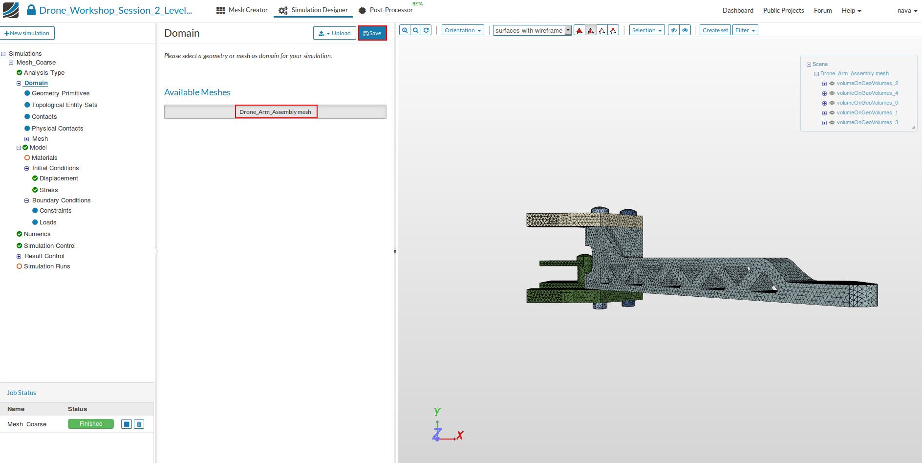
- Next you have to specify which mesh you want to use for your simulation. Click on Domain item in the project tree and select Drone_Arm_Assembly mesh from the menu and then Save.
- Select surfaces in Rendering mode to hide the mesh in the geometry.
Contacts
Since we are simulation an assembly of five parts it is necessary to define ** Contacts** which are describing the kinematic behaviour of the parts.
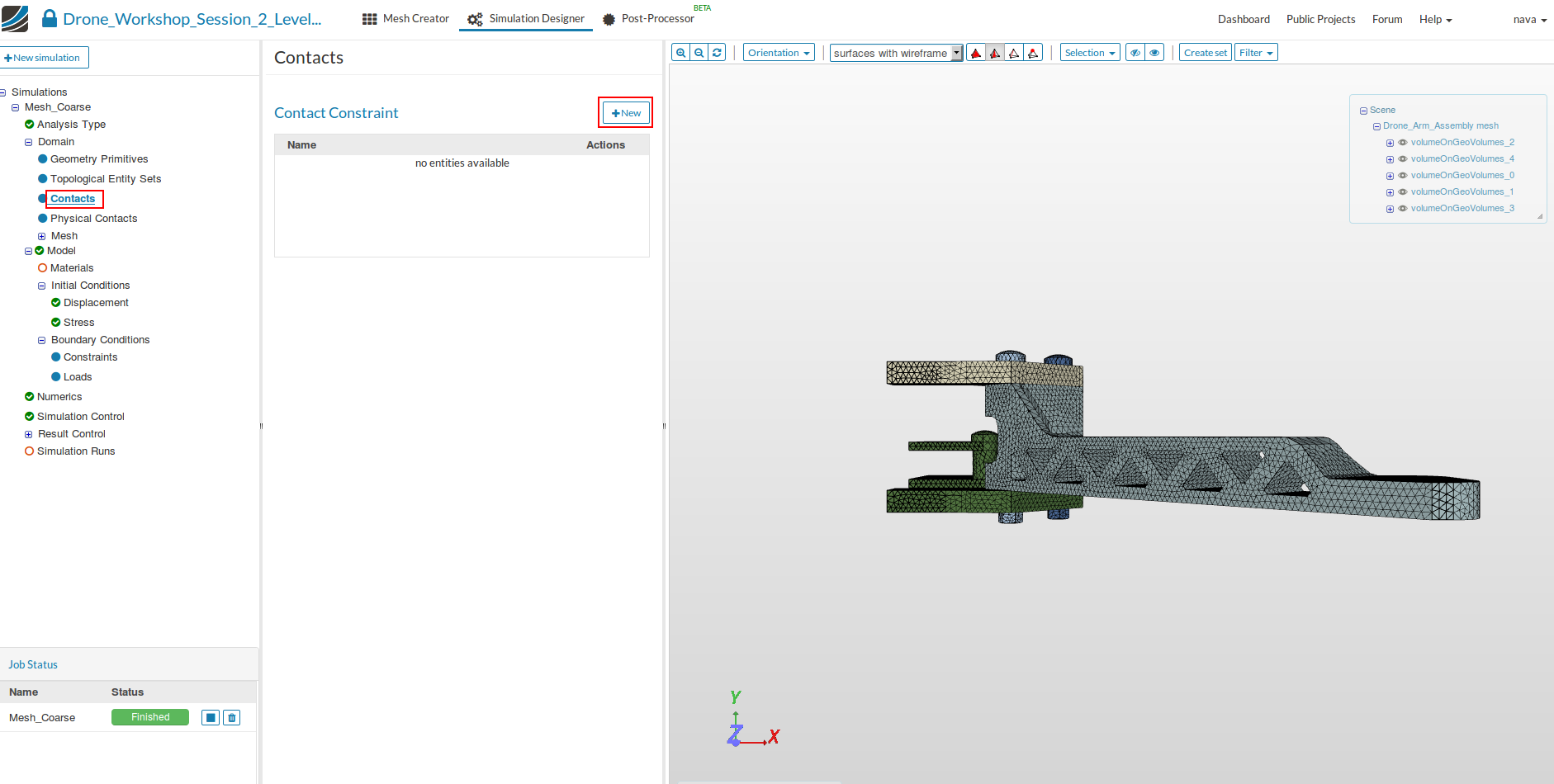
- Click on the Contacts item in the project tree which will open a new middle column menu where you can add new contacts by clicking on the New button.
- First hide the mesh in the geometry by selecting Surfaces in the rendering mode located at the Top menu.
![]() .
.
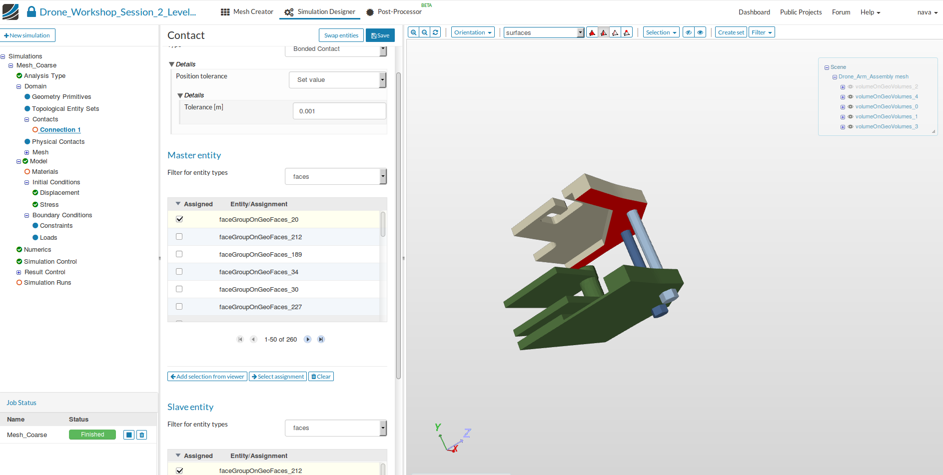
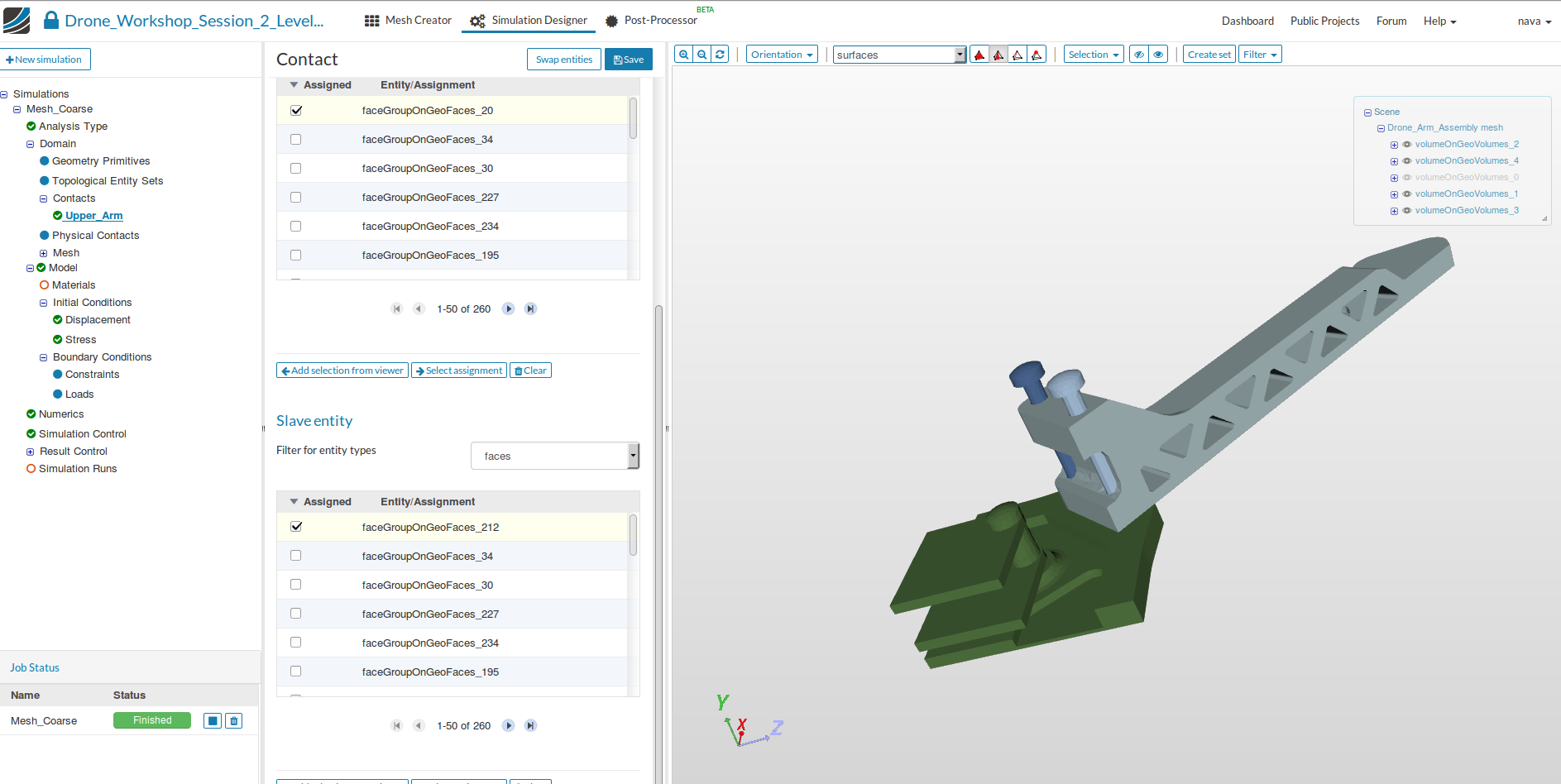
Now we have to create two contacts which are connecting the contact surface of the arm with the base plate. To select them graphically it is necessary to hide some of the parts.
Contact #1\
- Name: Upper_Arm (optional)
- Type: Bonded Contact
- Master entitiy: faceGroupOnGeoFaces_20
- Slave entity: faceGroupOnGeoFaces_212
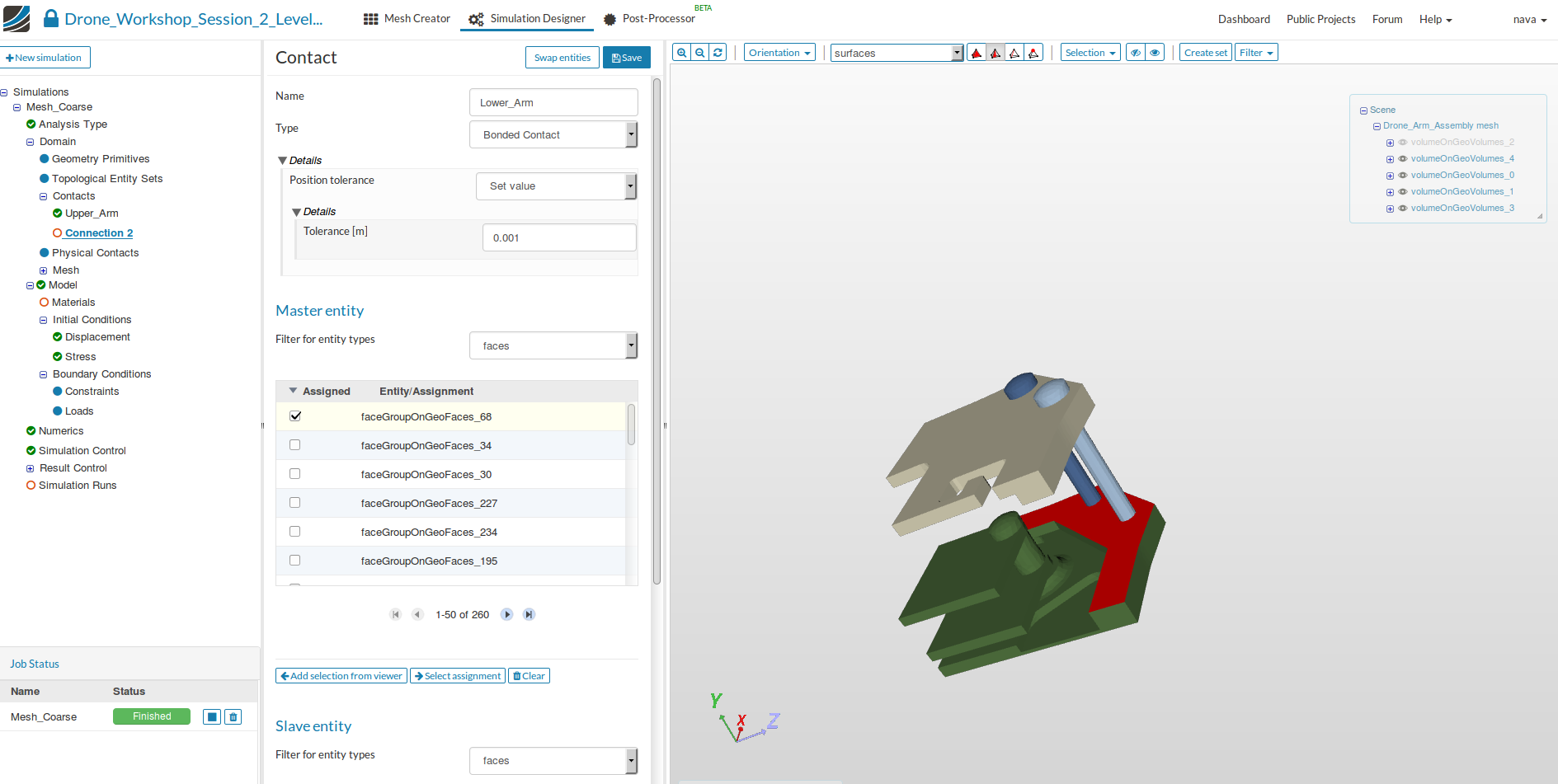
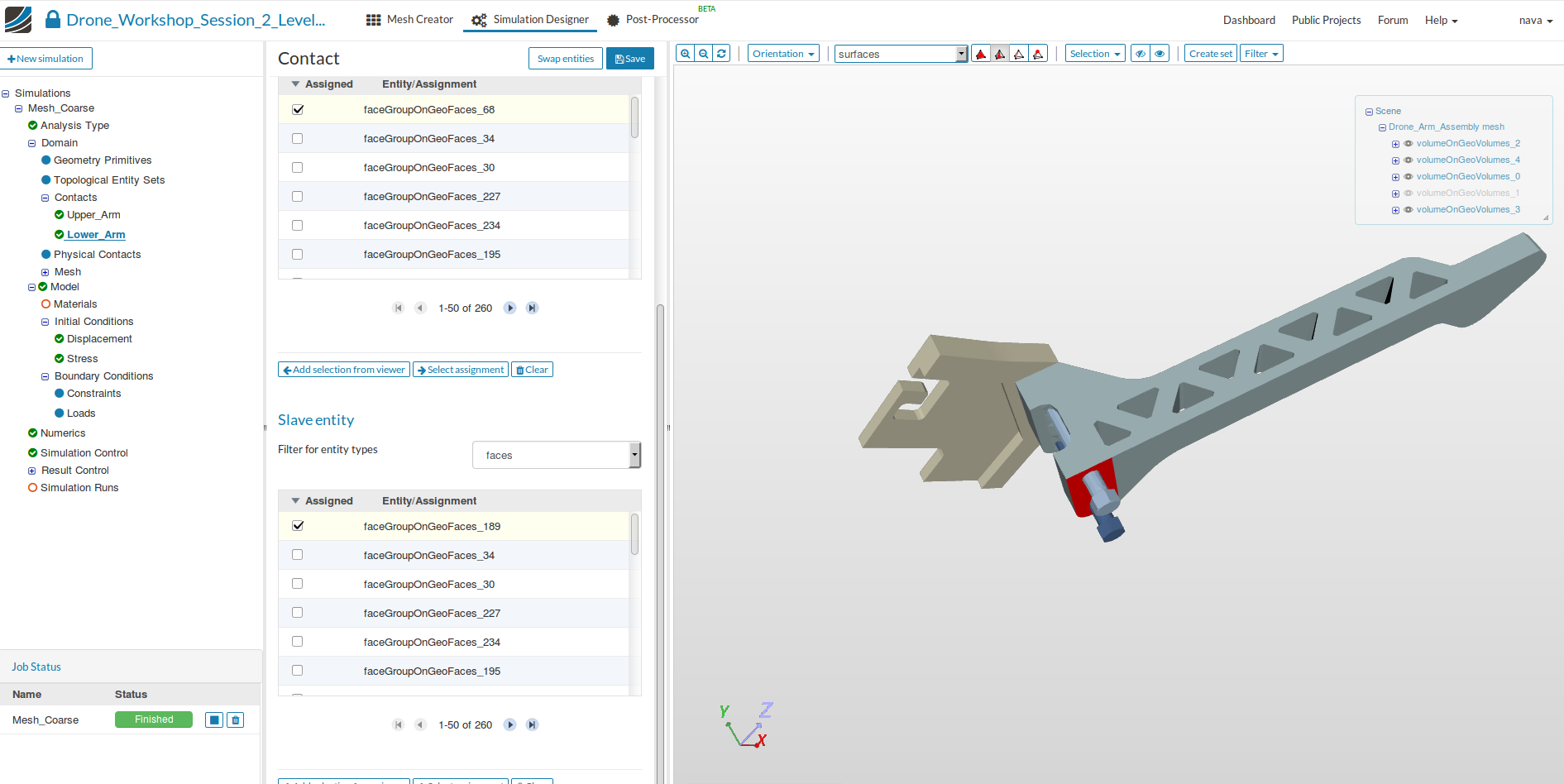
Contact #2
- Name: Lower_Arm (optional)
- Type: Bonded Contact
- Master entitiy: faceGroupOnGeoFaces_68
- Slave entity: faceGroupOnGeoFaces_189
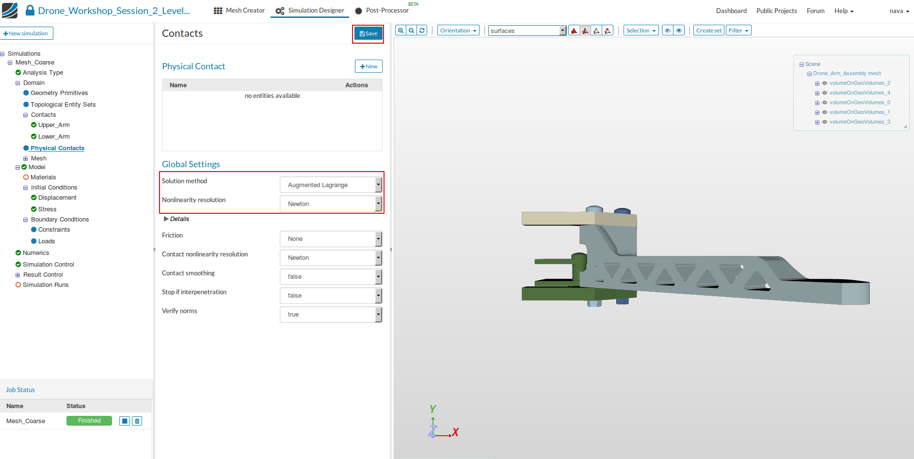
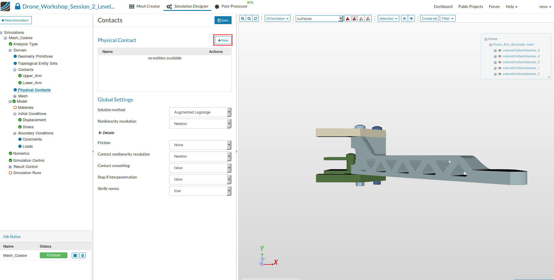
Physical Contacts
Next we will define the Physical Contacts. In contrast to Contacts, they are also covering the physical interaction between parts. We will use them to specify the contact between the head of bolt respectively the nut and the base plate.
- Click on the Physical Contacts item in the project tree. This will open a new middle column menu where we first will adapt two general settings:
- Solution method: Augmented Lagrange
- Nonlinearity resolution: Newton
- Save the settings.
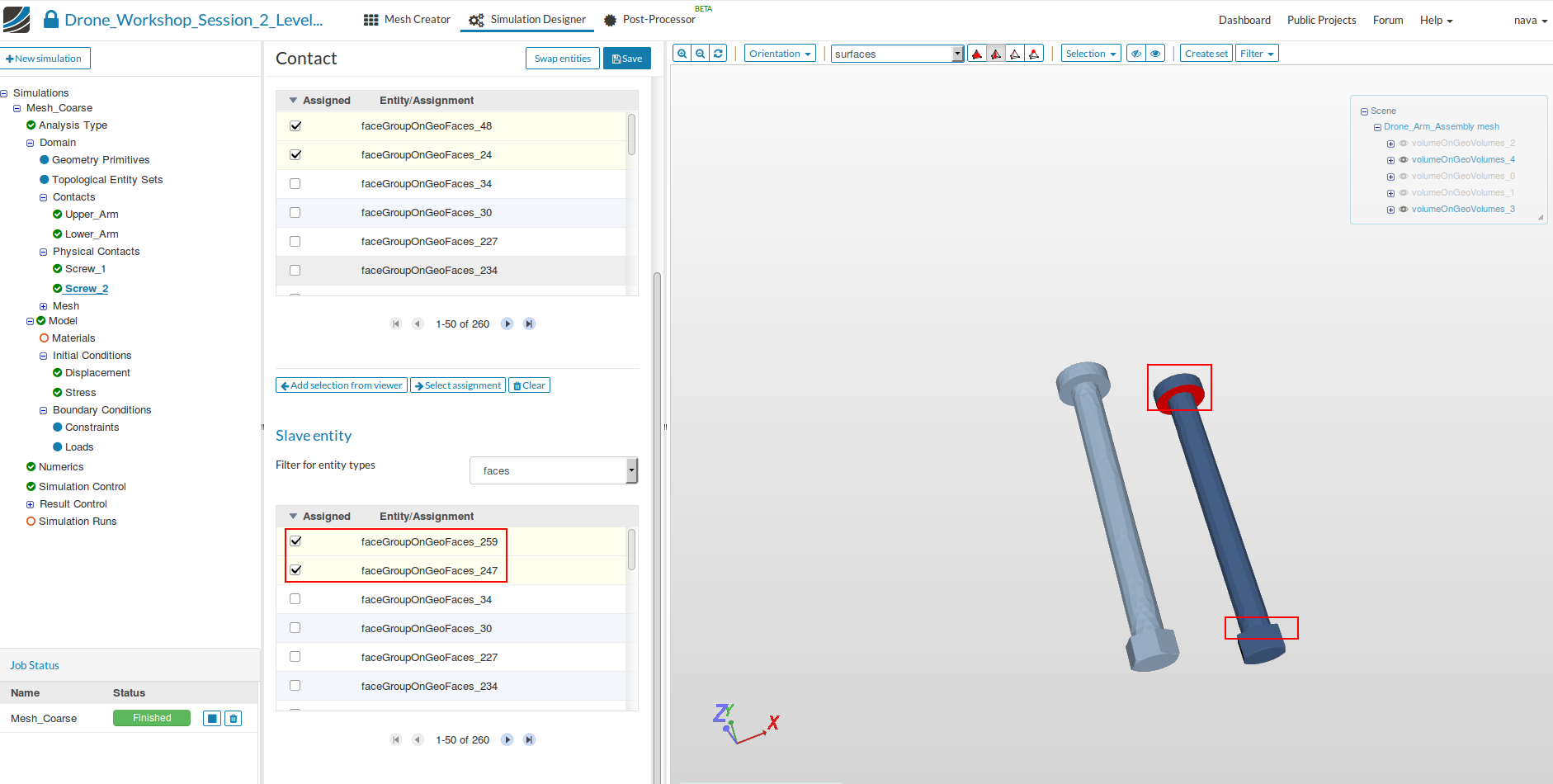
Now we will create a new contact by clicking the New button.
This will add a new contact to the project tree.
- Specify the following parameters:
- Name: Screw_1 (optional)
- Type: Frictionless augmented lagrange
- Master entitiy: faceGroupOnGeoFaces_35, faceGroupOnGeoFaces_46 (contact surface of the base plate with the screw connection)
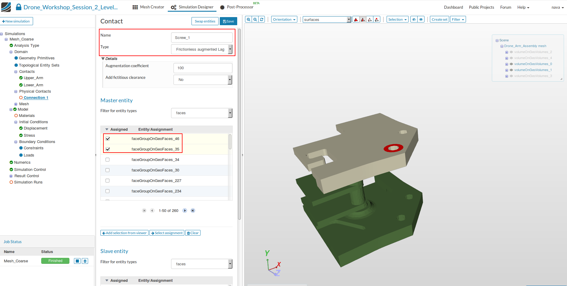
- Slave entity: faceGroupOnGeoFaces_225, faceGroupOnGeoFaces_237 (contact surface of the screw connection with the base plate)
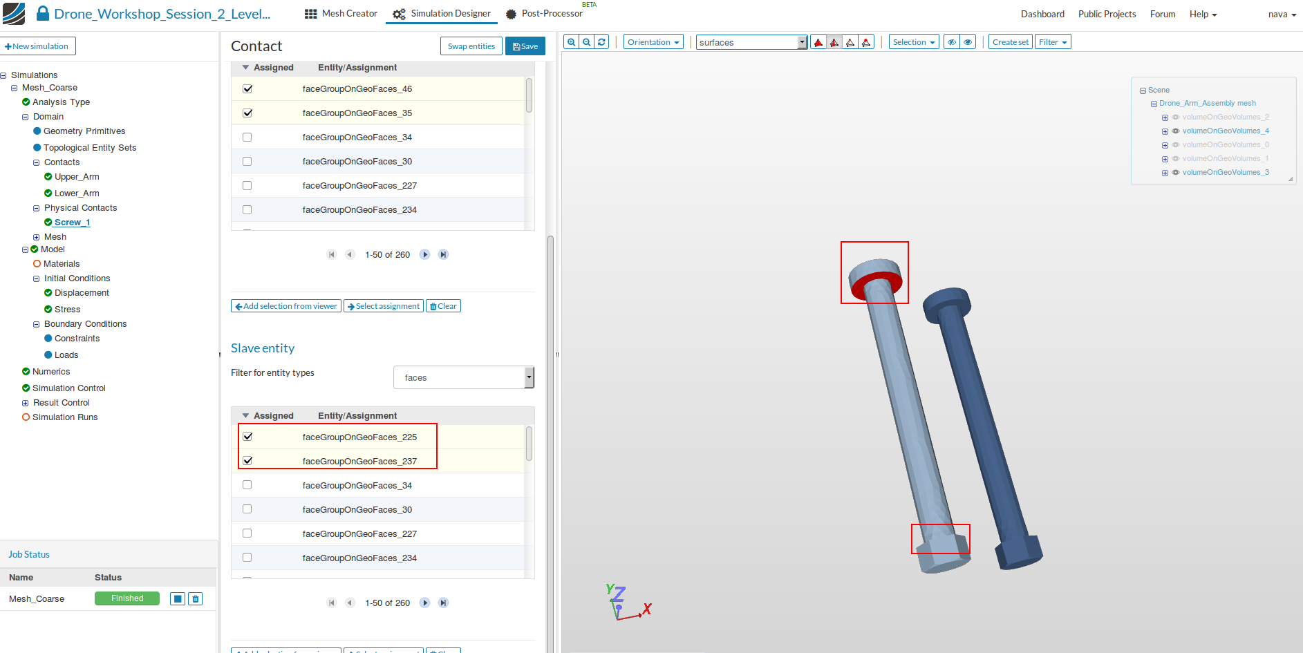
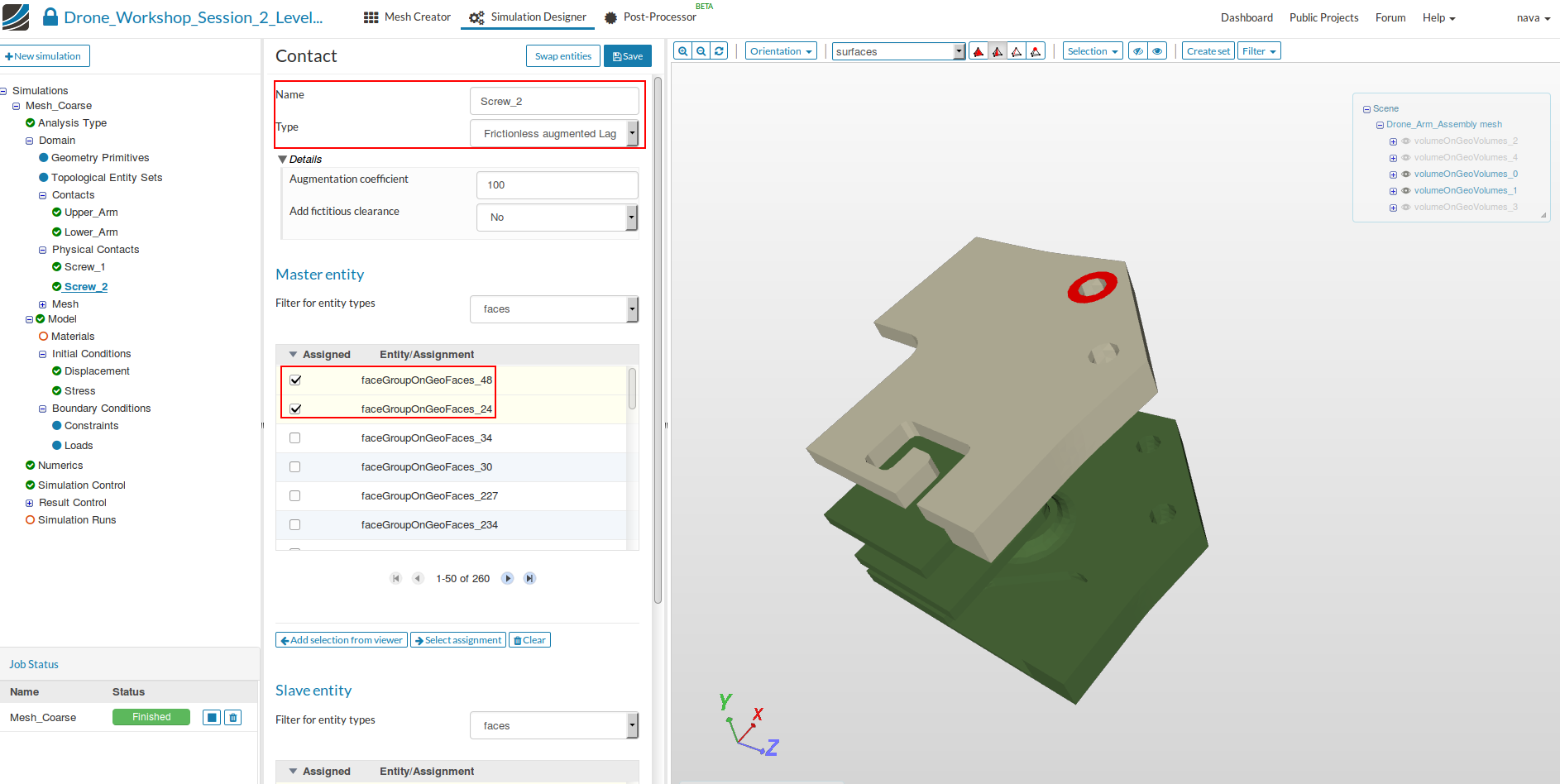
Please repeat the step for the other screw. The result should look like this:
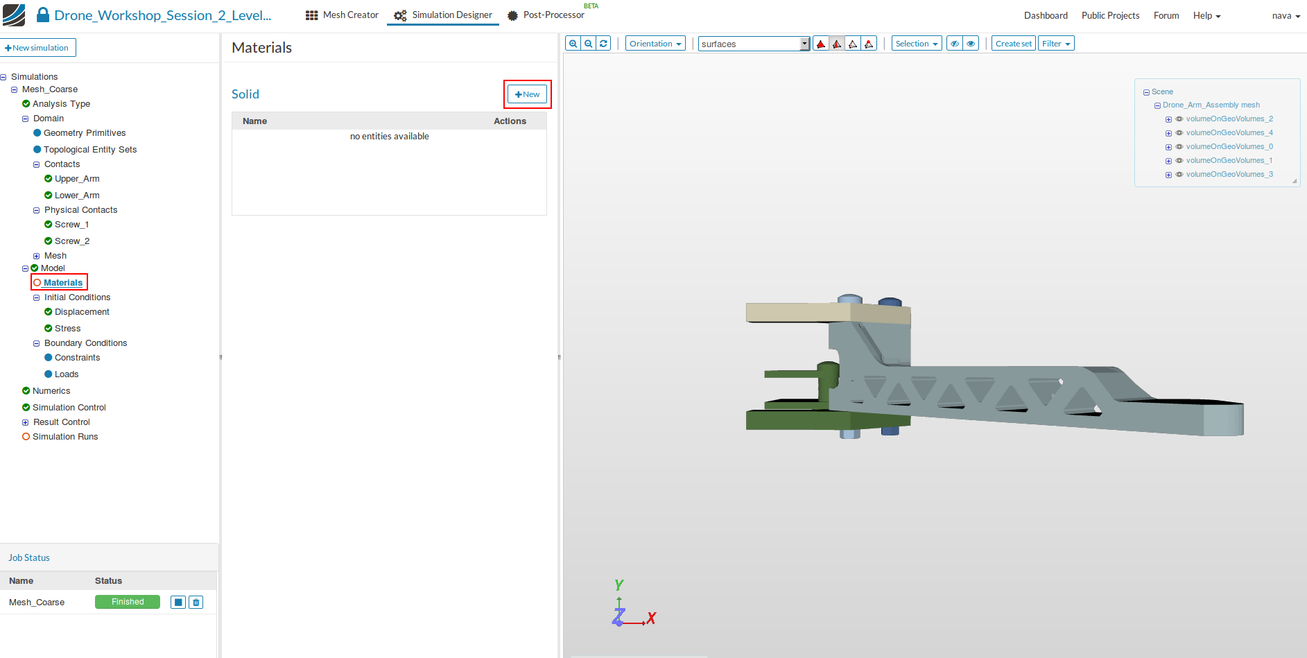
Select Solid Materials
Now we define and assign material properties to the different parts.
*Click on the Material item in the project tree. This will open a middle column menu where you can edit and create materials and assign them to volumes. Click on the New
Now you can define your new material based on your own material properties or access our *Material Library which includes ready-to-use material models for several materials.
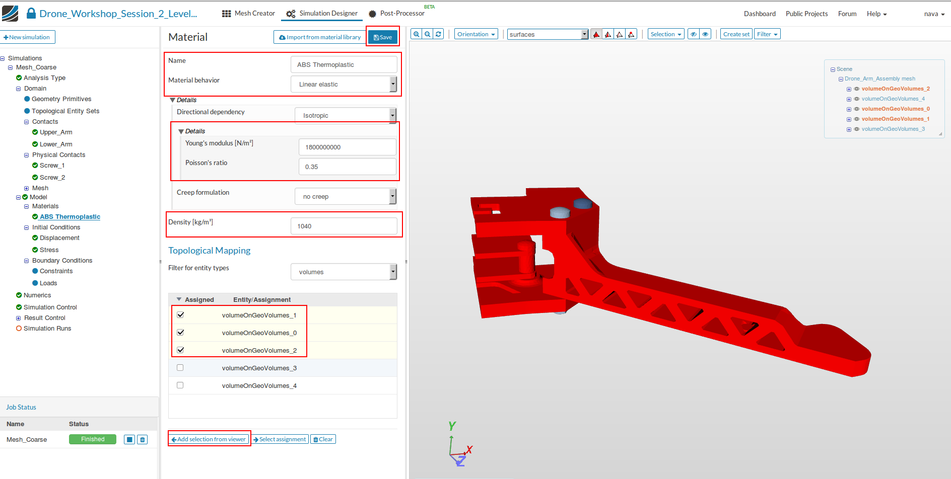
We will start with the manual definition of an ABS Thermoplastic.
- Specify the following parameters:
- Name: ABS Thermoplastic
- Young’s Modulus [N/m2]: 1800000000
- Poisson’s ratio: 0.35
- Densiy[kg/m3]: 1040
And assign in to all parts except the screw connection (volumeOnGeoVolumes_0, volumeOnGeoVolumes_1, volumeOnGeoVolumes_2)
- Save the settings.
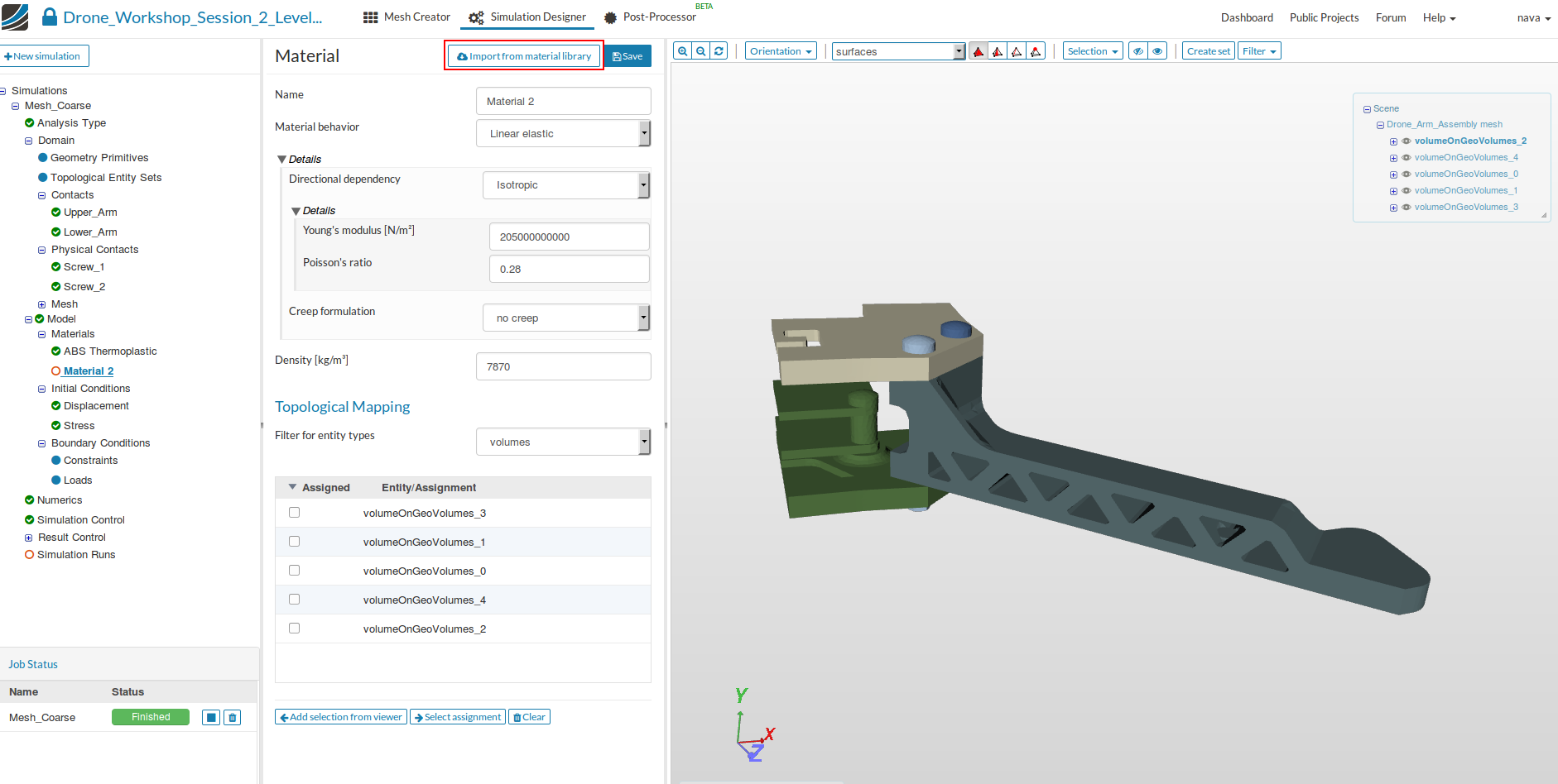
Next we will create and assign the steel material model to the screw connection.
- Add an additional material to your project tree by going back to Materials and then clicking on
New.
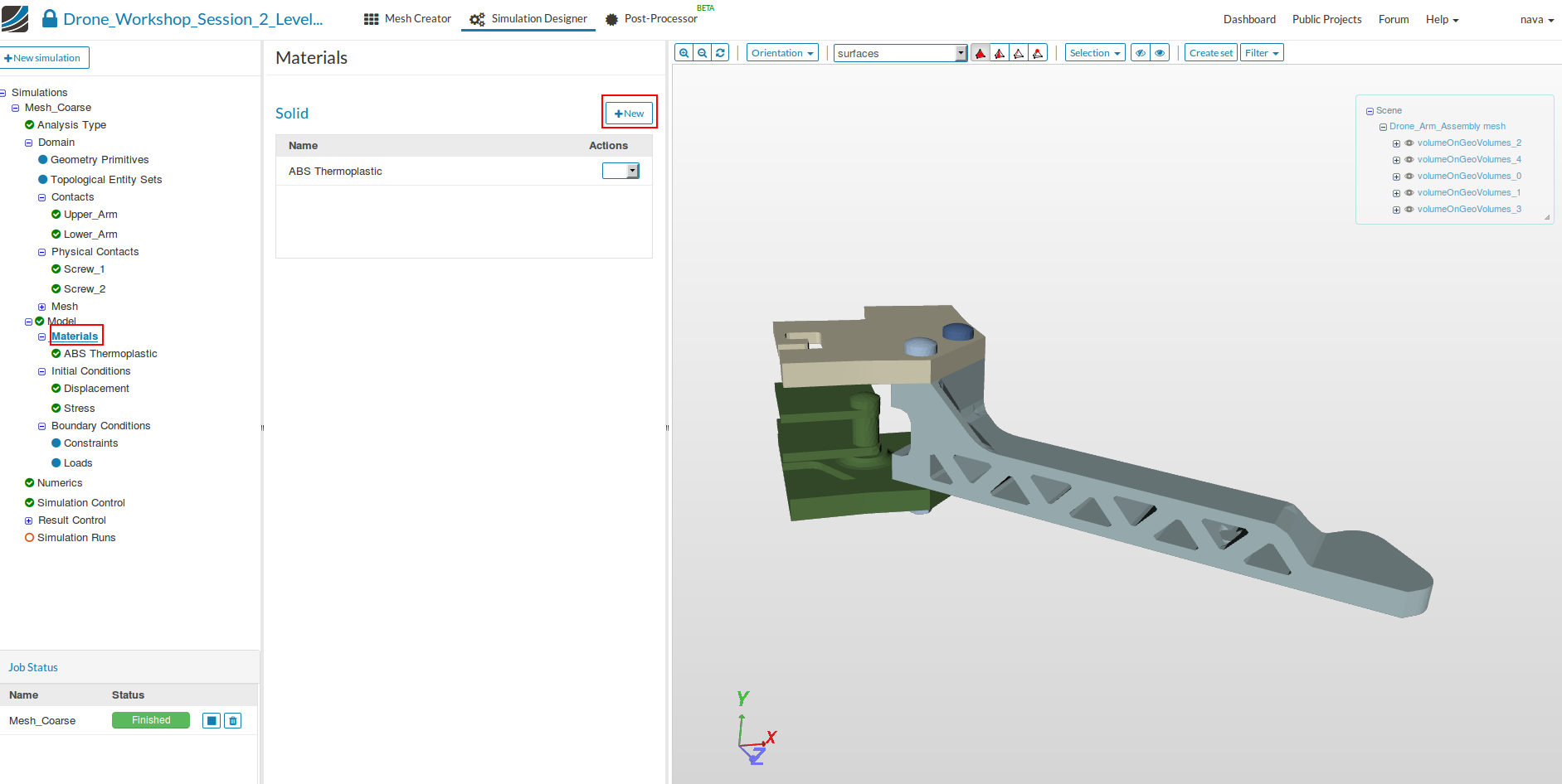
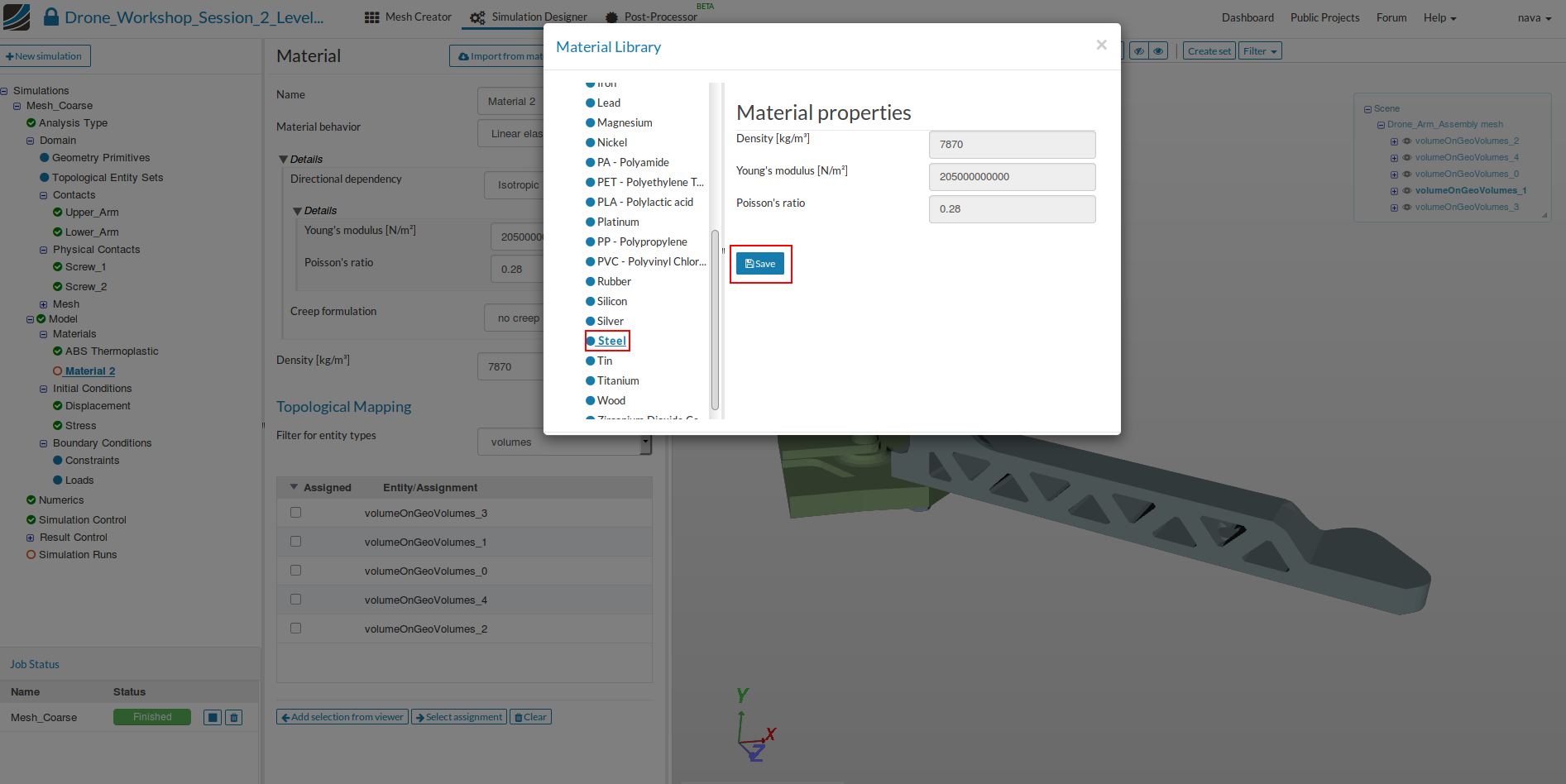
Now we will access our material library instead of creating the material model manually. Click on the Import from material library which will open a widget.
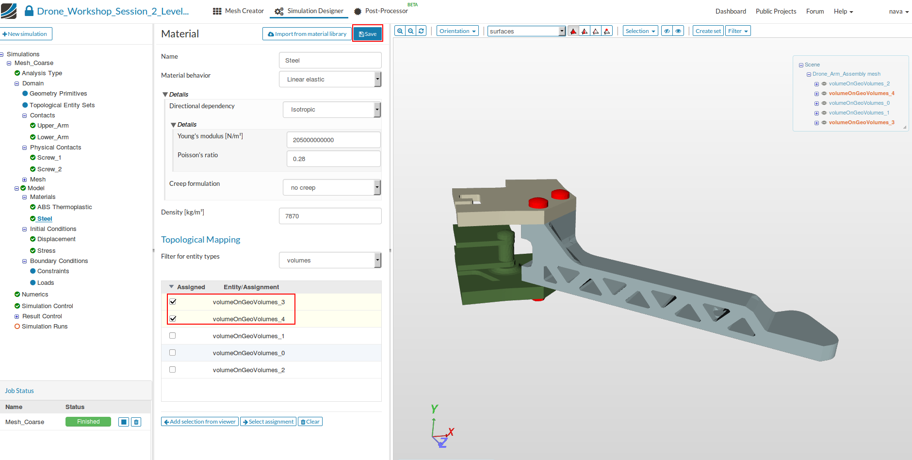
Please select steel from the list on the left side and save your selection by clicking on Save.
Now assign the material to the two screw connections (volumeOnGeoVolumes_3, volumeOnGeoVolumes_4)
Boundary Conditions
Next we can start to define the boundary conditions.
There are two kinds of boundary conditions for static structural simulations.
- Constraint conditions are used to limit the degrees of freedom of the model.
- Load conditions are applying an external load to the model
*First we will add four constraint boundary conditions which are needed.
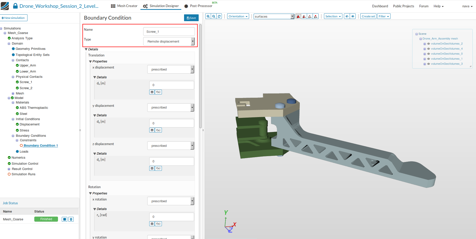
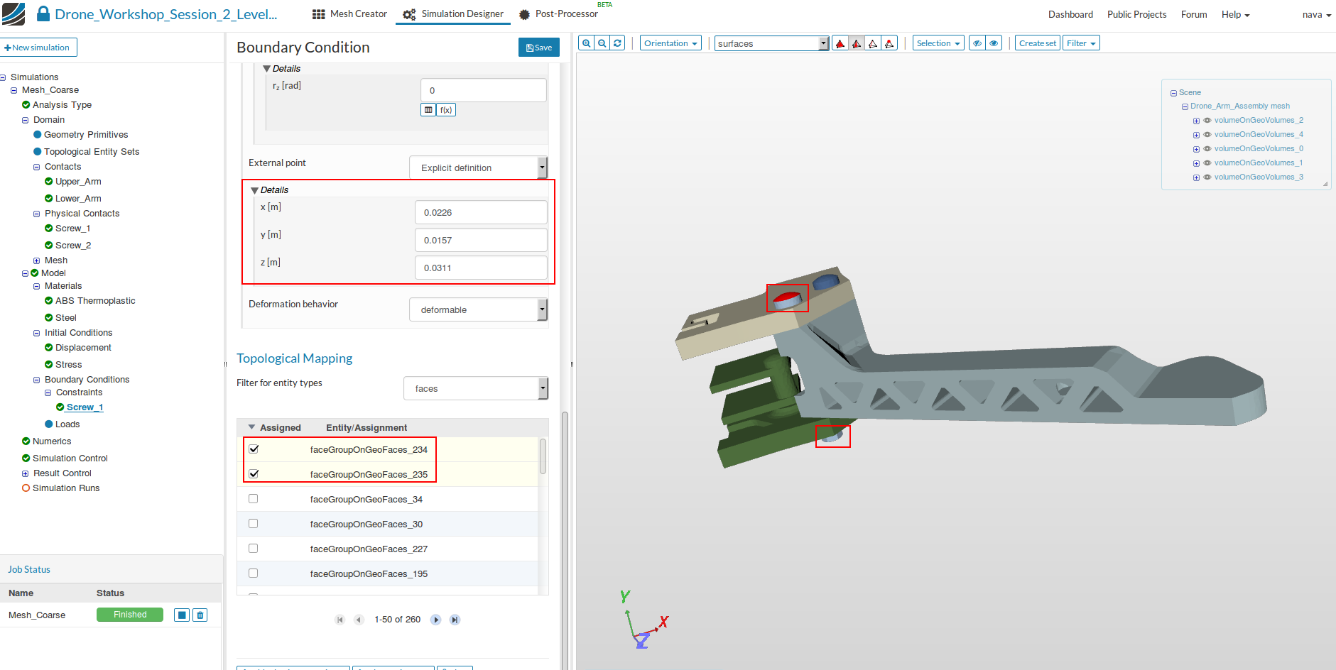
Screw_1
This bounday condition is necessary to define a relative reference point for the crew. We will define the centre of the screw as prescribed. This will make sure that the screw is stretching symmetrically.
-
Click therefore on the Constraint under Boundary Conditions in the tree and then click New.
-
Change the following parameters:
- Name: Screw_1
- Type: Remote displacement
- Translation: All displacements (x, y, z) are prescribed with a value of 0
- Rotation: All rotations (x,y,z) are prescribed with a value of 0
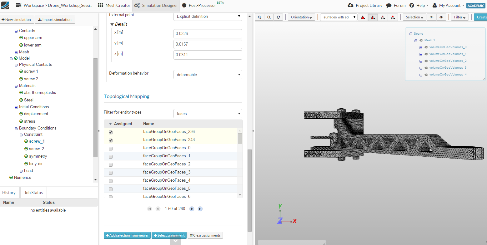
- External point: Explicit definition´
- x [m] = 0.0226
- y [m] = 0.0157
- z [m] = 0.0311
-
Deformation behavior: deformable
-
Finally map this boundary condition to the two opposite faces of the screw head (faceGroupOnGeoFaces_234, faceGroupOnGeoFaces_235) and then click on Save to save yoru settings.
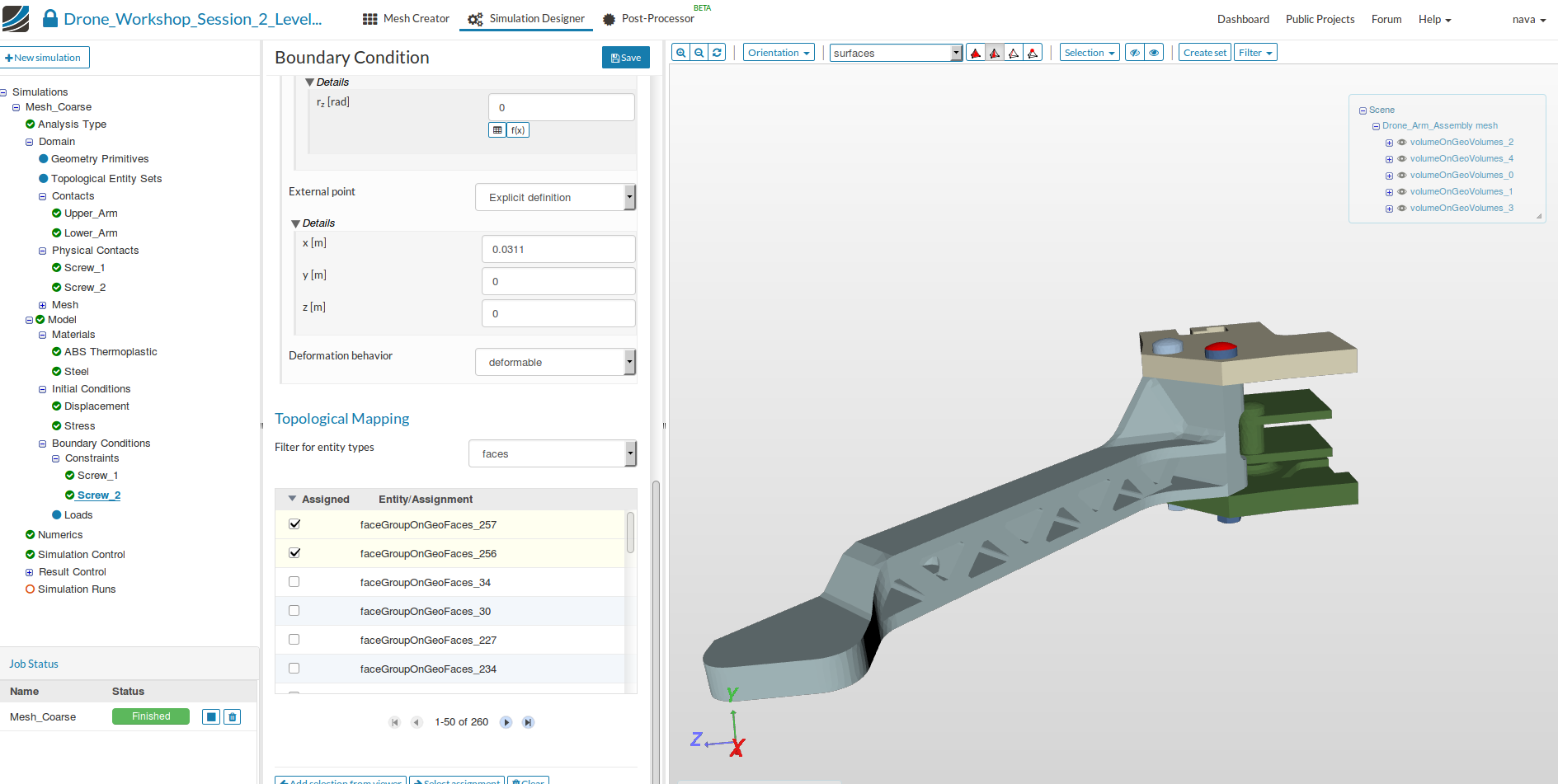
Screw_2
The role of this boundary conditions is similar to Screw_1 but related to the second screw.
- Change the following parameters:
- Name: Screw_2
- Type: Remote displacement
- Translation: All displacements (x, y, z) are prescribed with a value of 0
- Rotation: All rotations (x,y,z) are prescribed with a value of 0
- External point: Explicit definition
- x [m] = 0.0311
- y [m] = 0.0157
- z [m] = 0.0226
- Deformation behavior: deformable
- Finally map this boundary condition to the two opposite faces of the screw head (faceGroupOnGeoFaces_256, faceGroupOnGeoFaces_257) and save your settings by clicking on Save.
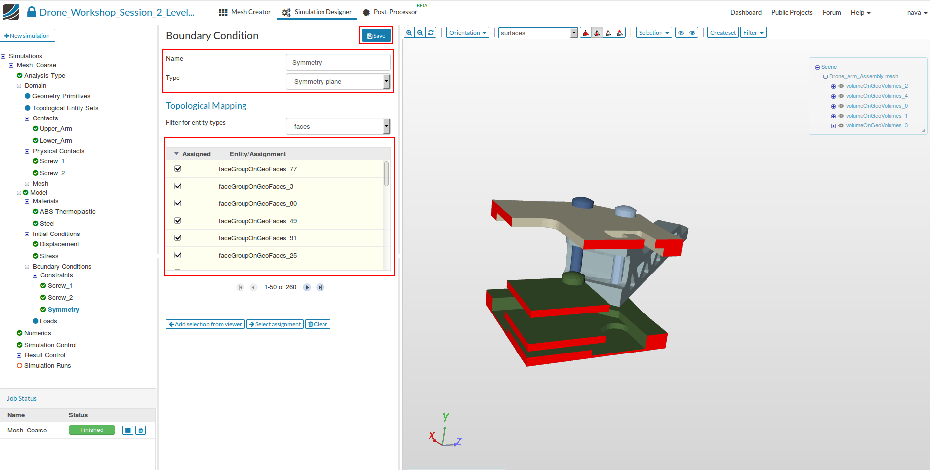
Symmetry
This boundary condition is required because we are using a quarter model of the drone.
Create a new constraint boundary condition by clicking the New button after going back to Constraints in the project tree.

- Change the following parameters
- Name: Symmetry
- Type: Symmetry Plane
- Please assign all surfaces of the drone base plates which are bounding with the two imaginery symmetry planes and therefore behaving like a symmetry plane (faceGroupOnGeoFaces_25, faceGroupOnGeoFaces_32, faceGroupOnGeoFaces_49, faceGroupOnGeoFaces_50, faceGroupOnGeoFaces_77, faceGroupOnGeoFaces_80, faceGroupOnGeoFaces_90, faceGroupOnGeoFaces_91, faceGroupOnGeoFaces_3)
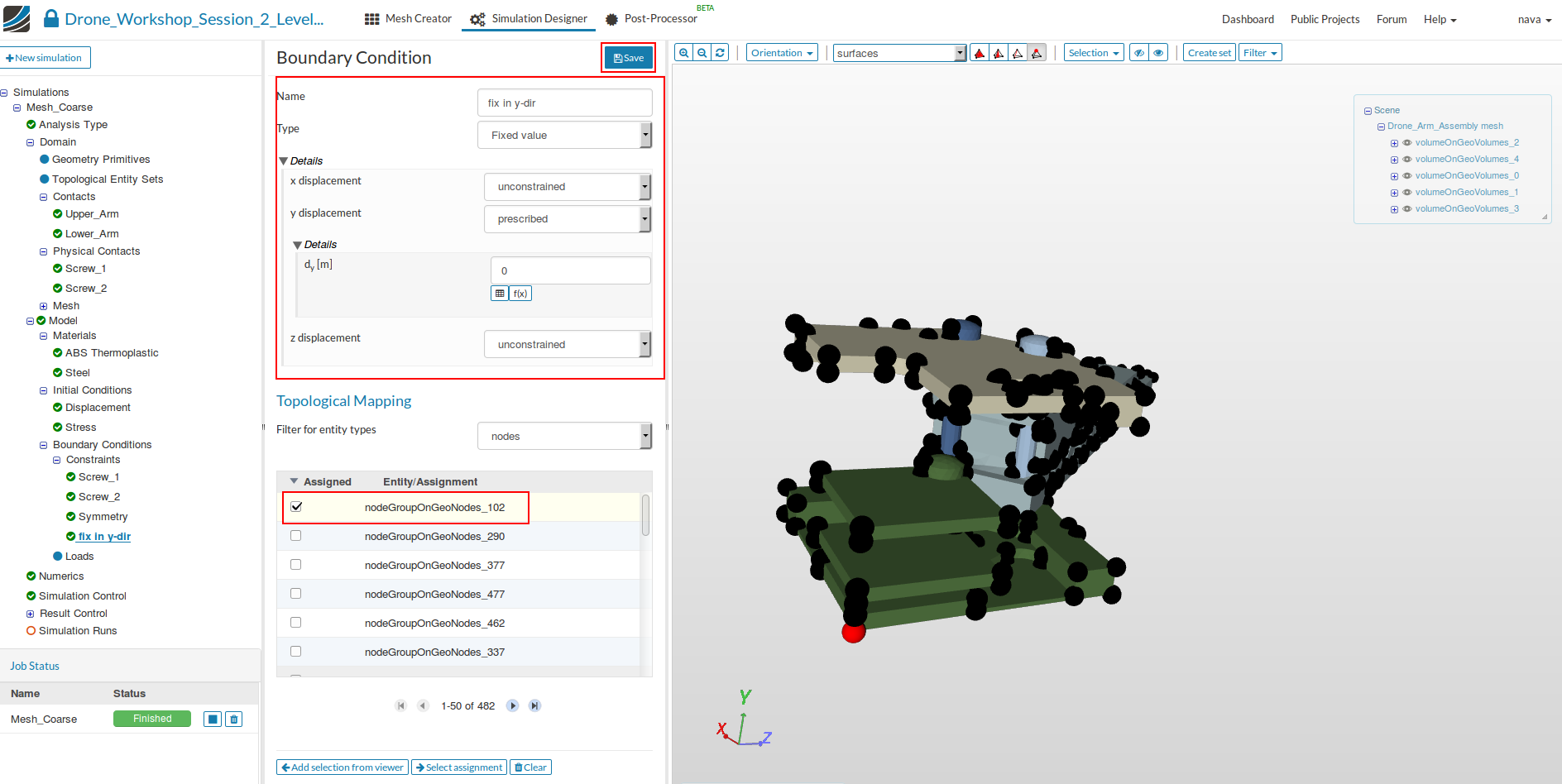
Fix in y-dir
The last constraint boundary conditions we have to define is a fixiation in Y direction. This is only necessary for Y direction since the model is already fixed in X and Z direction by the symmetry plane boundary condition.
-
Create a new constraint boundary conditions following the step mentioned above.
-
Change the following parameters:
- Name: fix in y-dir
- Type: Fixed value
- x displacement: unconstrained
- y displacement: prescribed with a value of 0
- z displacement: unconstrained
In contrast with the other three boundary conditions, we will map this one only to a single node of the model. For graphical selection you have to change the selection mode to nodes.
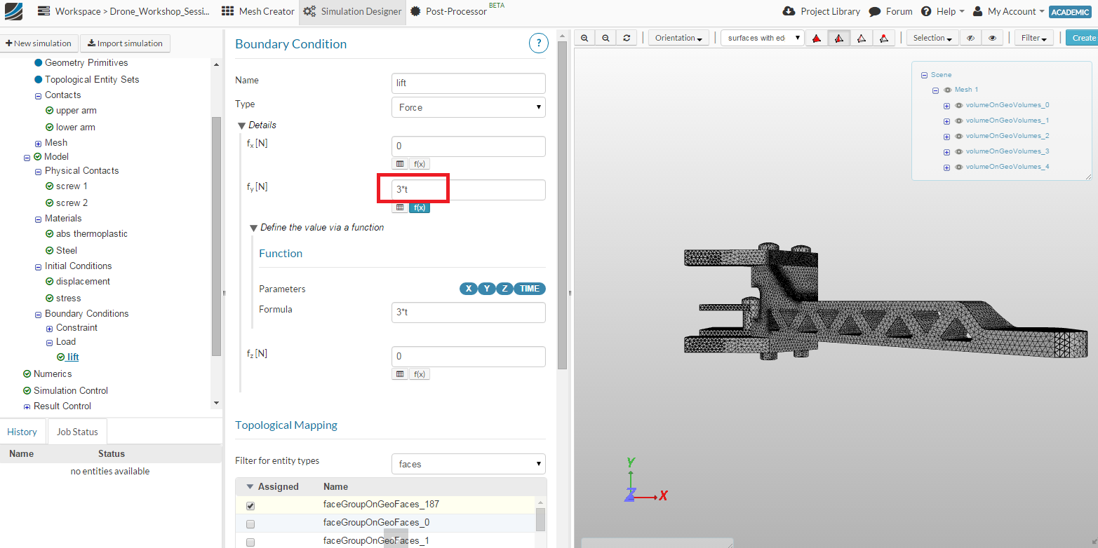
Lift
We are now on the home straight. We will apply the lift created by the propeller on the arm. We therefore apply load boundary condition.
Create a new Load boundary condtion by clicking on New button after to going to the Load entry in the project tree.
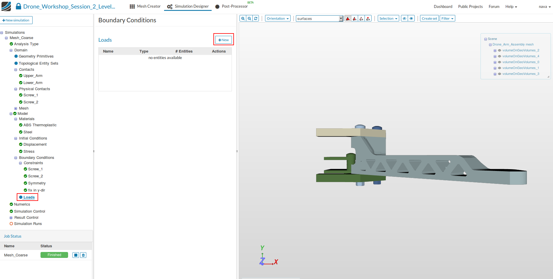
- Change the following parameters:
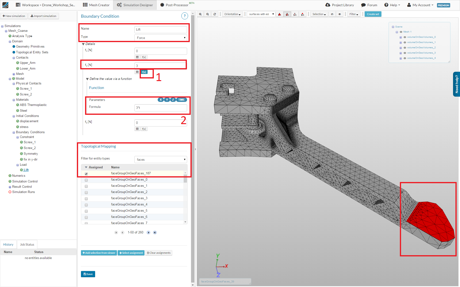
- Name: Lift
- Type: Force
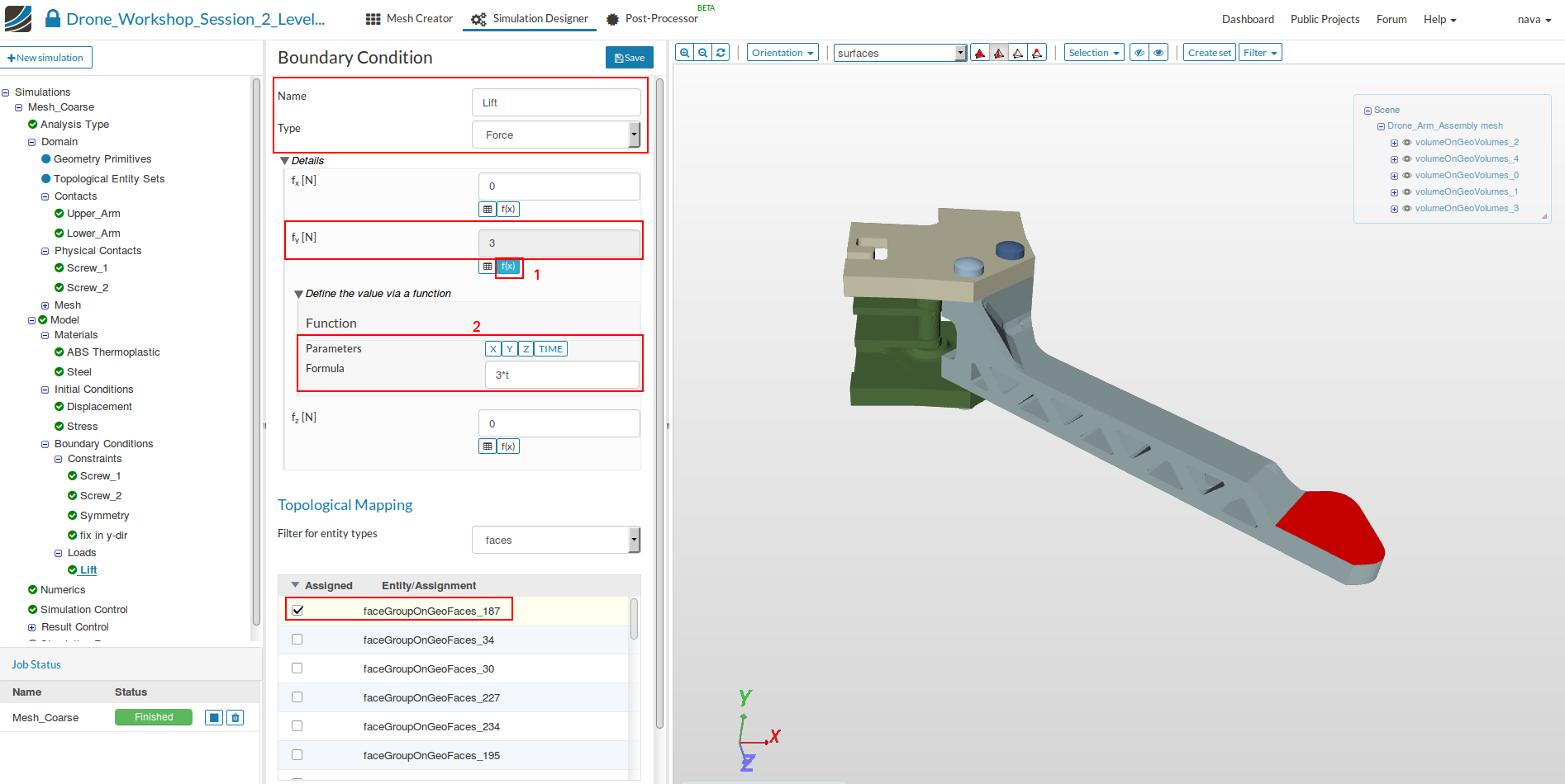
Again, in this tutorial we want to investiagte and compare several values for the lift force. Instead of creating four different simulations, we will use a smart work flow.
-
Define a force of 3N in Y direction and click on the small function button below the field (1). That will open a new field (2) where you have to enter the following Formula: 3*t. This will increase the force for every Timestep (t) and create for every of this forces a dedicate simulation result.
-
Finally assign this boundary condition to the top surface of the engine mount.
Numerics, which is the next item in the project tree, can be skipped since the default settings are fine.
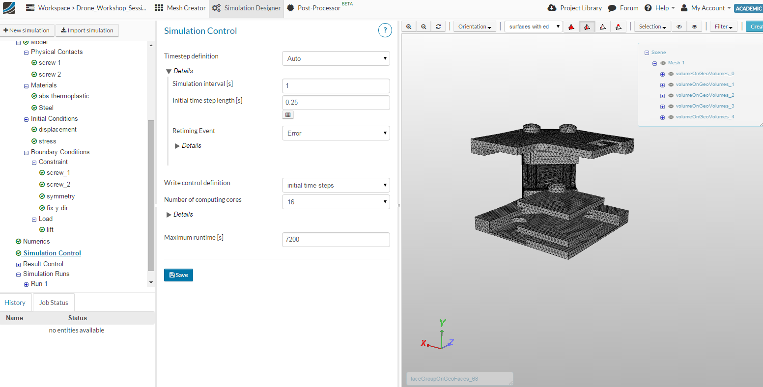
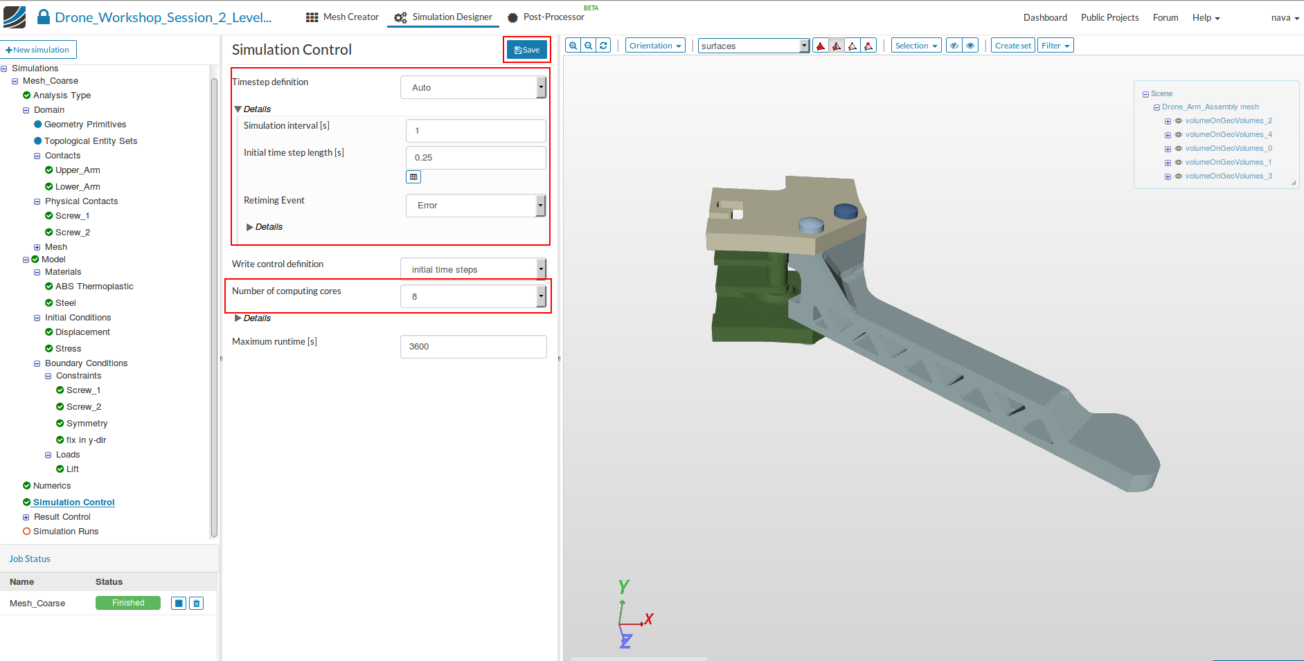
Simulation Control
Click on the Simulation Control item in the project tree to specify how fast and accurate you want the simulation to be computed.
- Change following values/settings:
- Timestep definition: Auto
- Simulation interval: 1
- Initial time step lengths: ** 0.25**
- Number of computing cores: 8 (that will accelerate the computing process)
Please note that static linear simulations are not solved iteratively. The simulation time here is a kind of ‘pseudo-time’ which is for example used to modify the lift force based on the function we defined. The calculation will stop automatically when an aimed residual is reached.
Result Control
- Click on the Result Control item in the project tree which will open a new middle column menu.
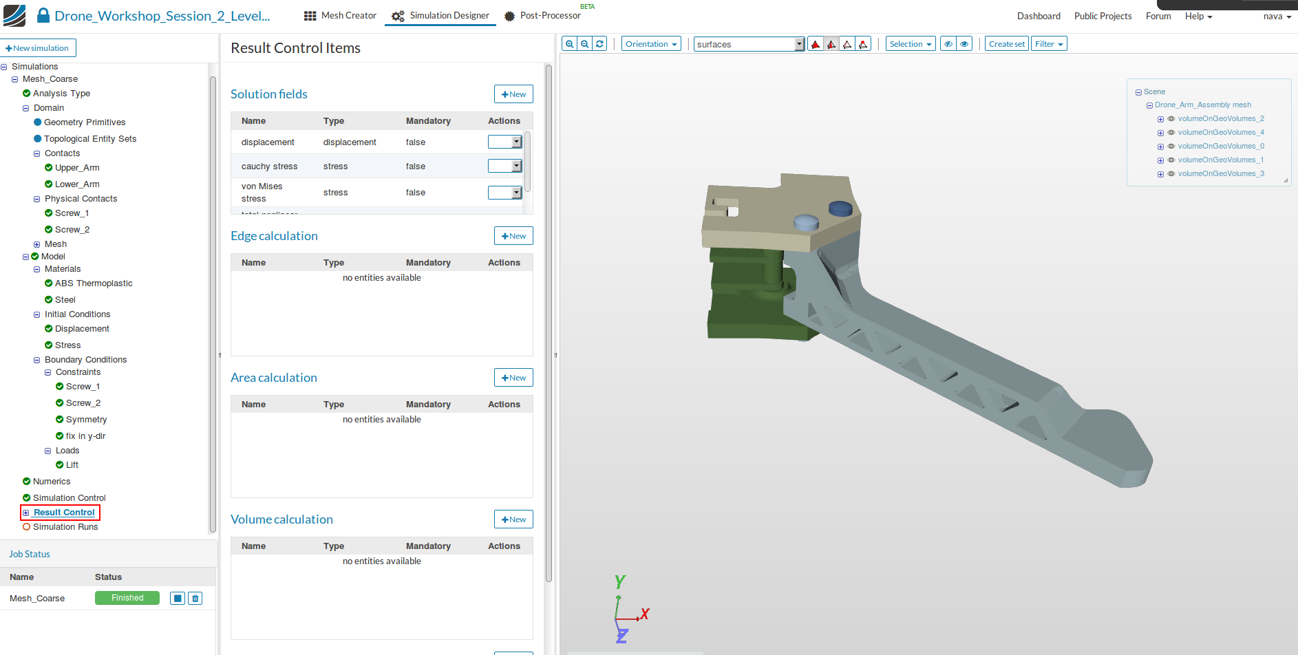
- Click on the New button near *Edge calculation
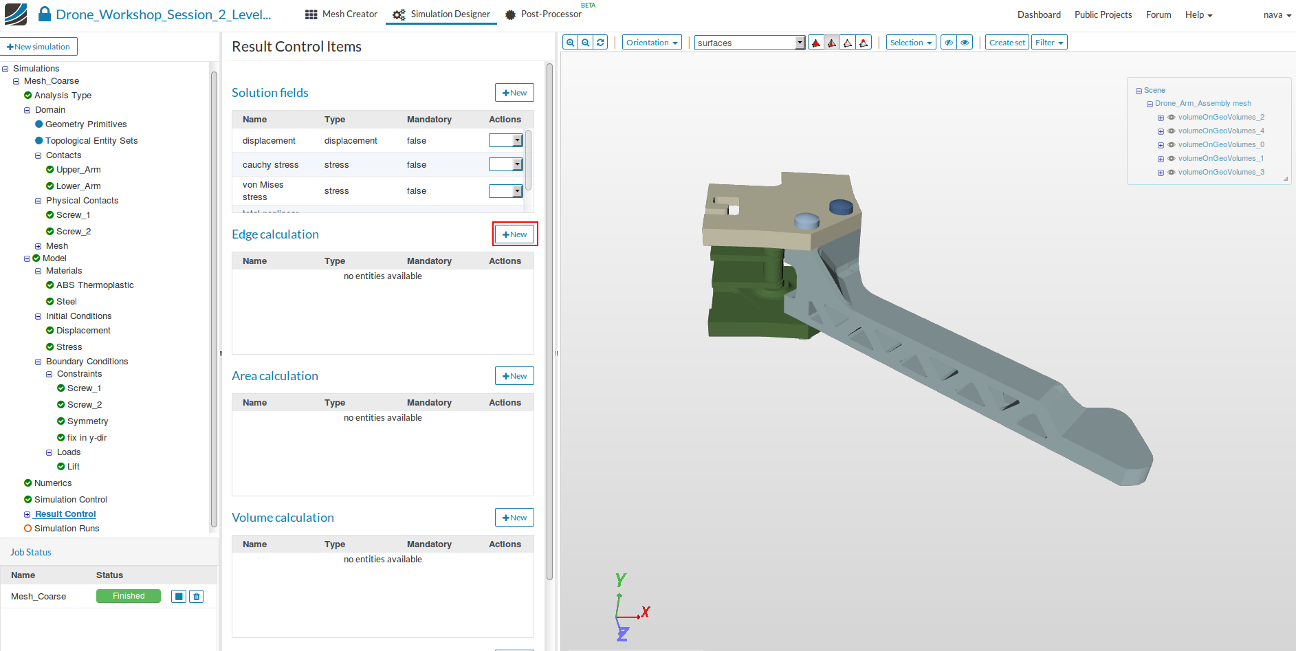
- Now define the Result Control item as follows:
- Name: Arm
- Type: average
- Field selection: displacement
- Component selection: y displacement
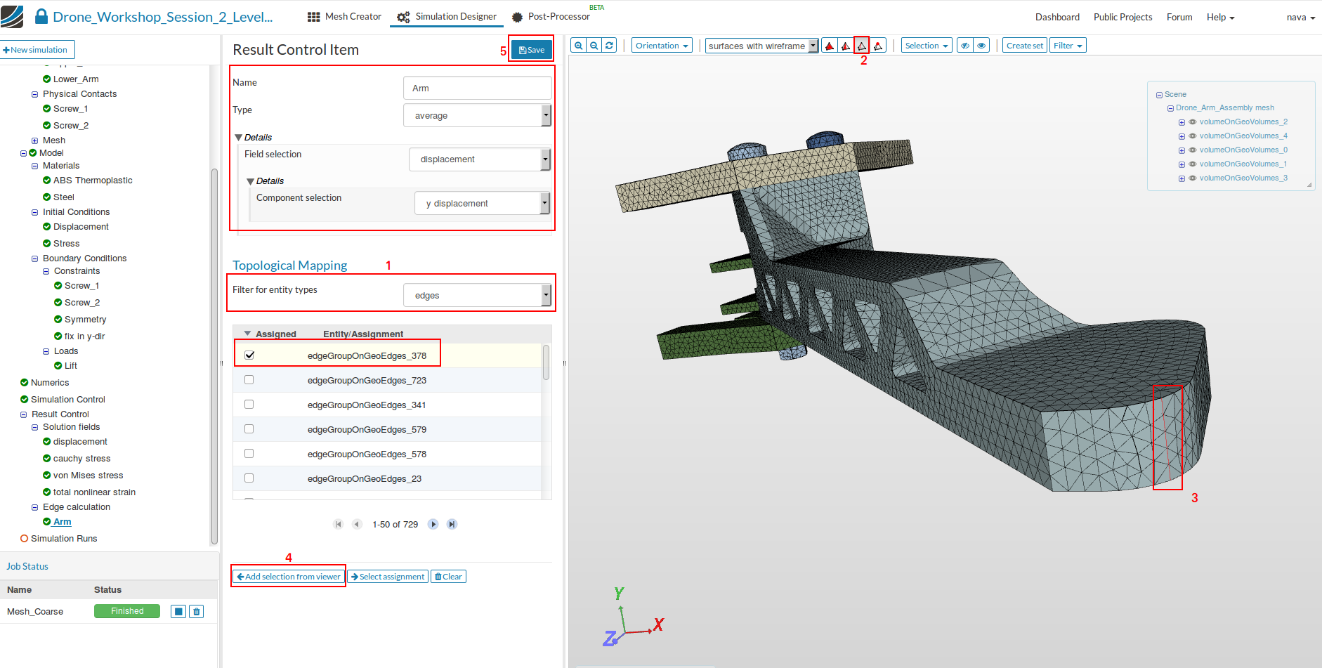
- Map it to the leading edge of the arm (edgeGroupOnGeoEdges_378) by first changing the render mode to surface with wireframe and choose edges for Filter for entity types (1).
- Change the selection mode to Edges (2) and select the leading ege (3) and click Add selection from viewer (4).
*Click Save to save all settings (5).
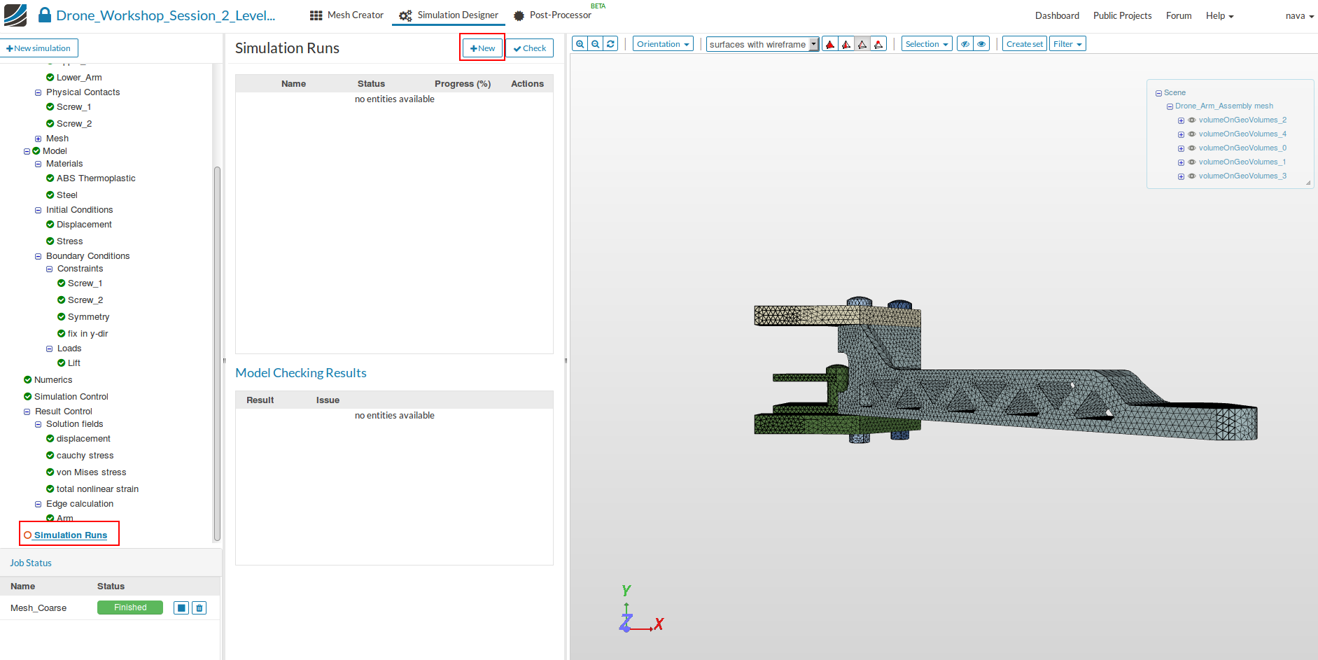
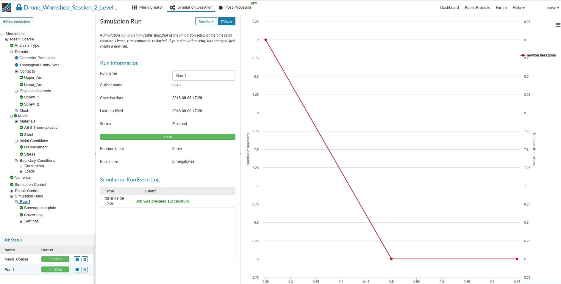
Simulation Runs
- To start the simulation, click on the Simulation Runs item in the tree and click on the New button.
You can now start the simulation run by selecting it from the project tree and then click on the Start button.
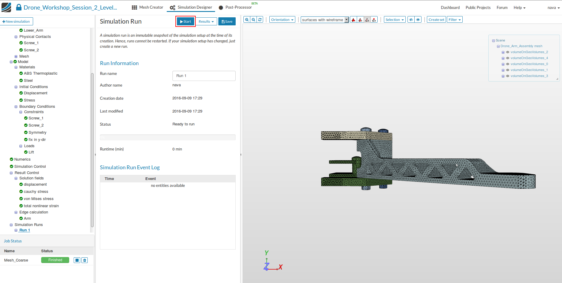
- Once your simulation is finished, you will see a Finished status in the lower left corner.
Post-Processing
- Click on Post-processing tab.
First of all we will take a look at the Result Control item we added.
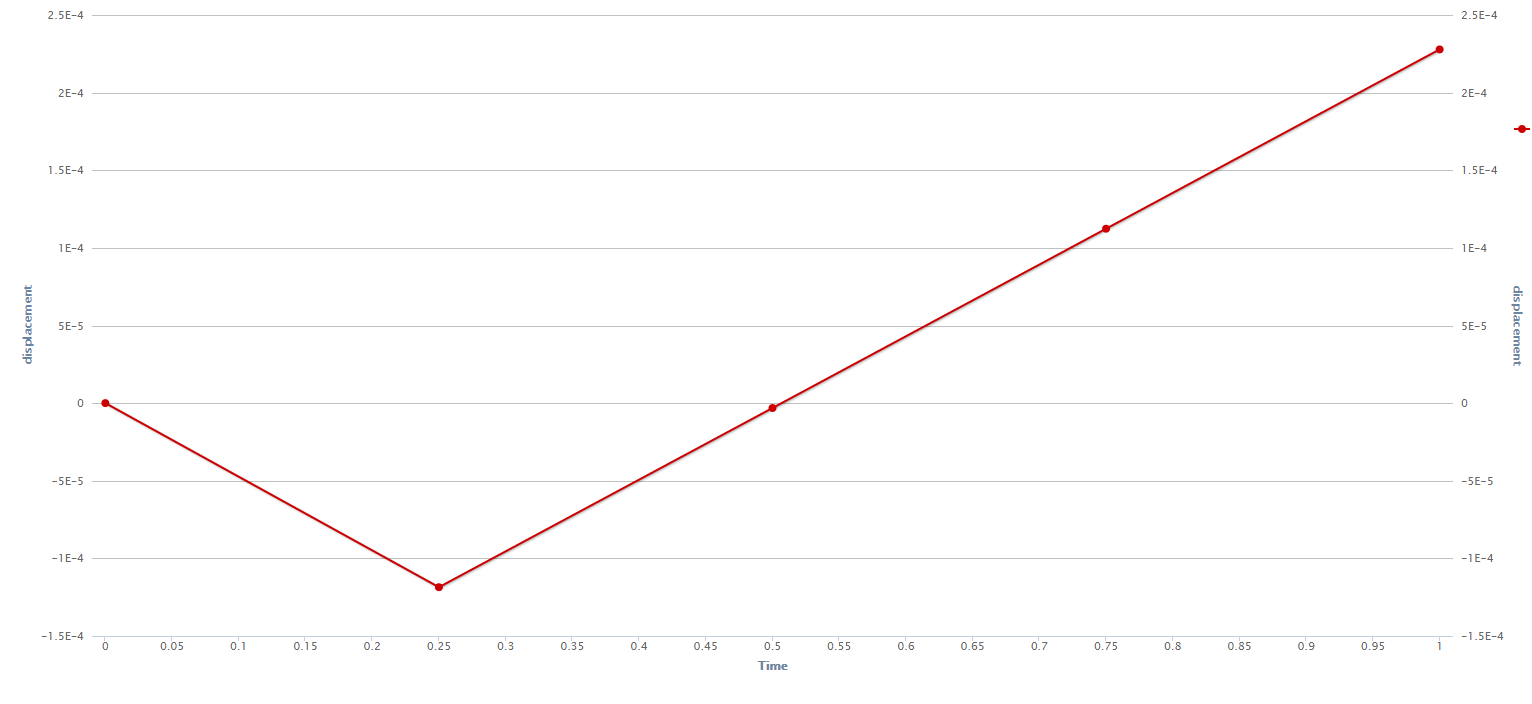
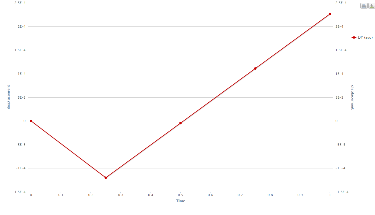
- Expand the Edge calculation item in the project tree and click an the lowest element.
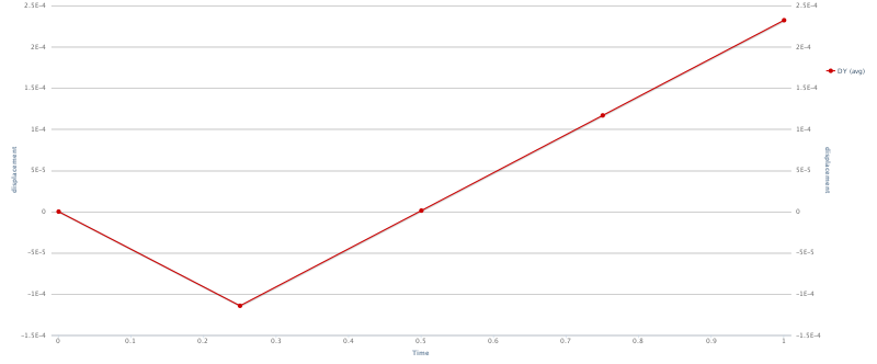
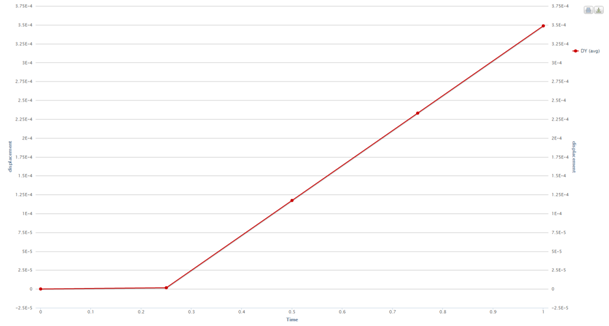
This will plot the change of average displacement for the arm versus the ‘Time’ which is equal to the lift force. The graph shows how the displacement is increasing with the force.
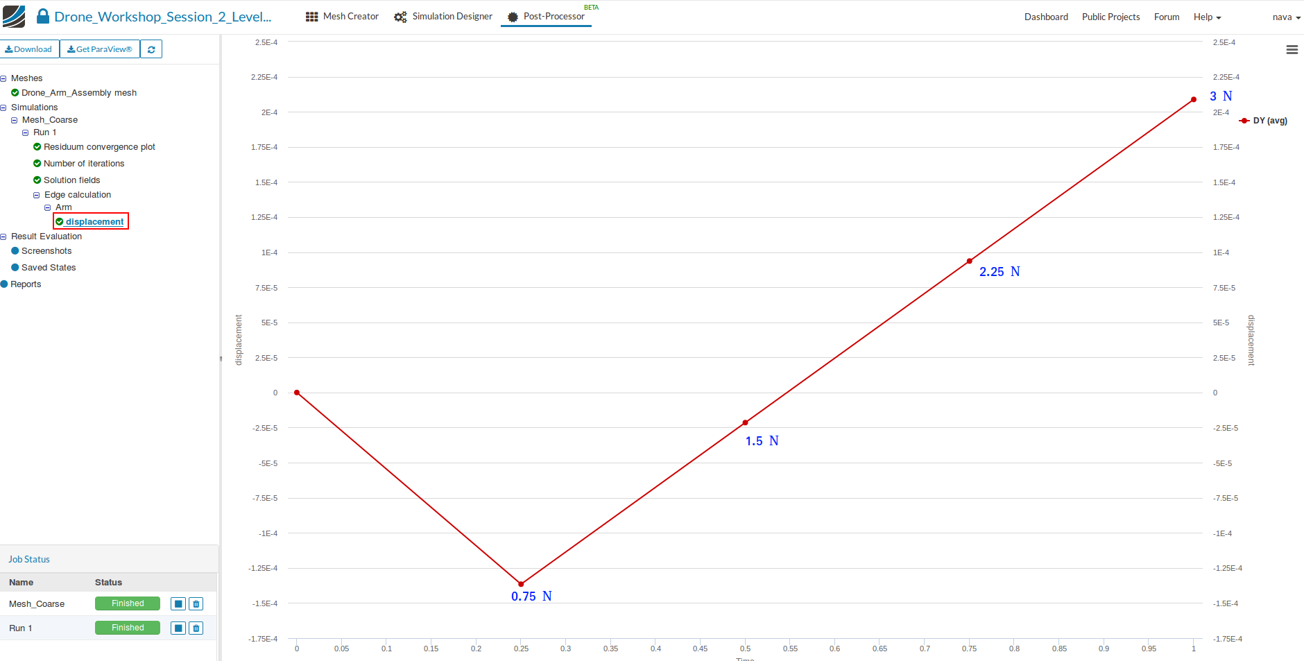
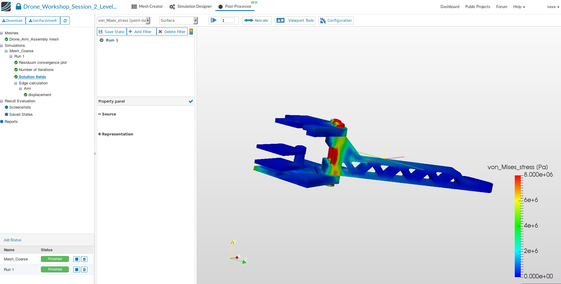
- Next we will take a look at the 3D result. Click on the Solution fields in the project tree. Now you can perform the solution field post-processing. Please use the instructions of Level 1.
Keep in mind that this simulation contains four load cases. This is why you can switch between this loads by using the related time step (0.25 = 0.75N, 0.5 = 1.5N, 0.75=2.25N, 1 = 3.0N)
- To complete this level please repeat the meshing and simulation setup for the same geometry with a higher refinement:
Screws Refinement
- Maximum mesh edge length: 0.0004
- Minimal mesh edge length: 0.00002
- NETGEN3D fineness parameter: 3 - Moderate
High Stress Zone Refinement
- Name: High Stress Zone Refinement
- Maximum mesh edge length: 0.00015
- Minimal mesh edge length: 0.00005
- NETGEN3D fineness parameter: 3 - Moderate
Congratulations, you have completed the Homework of Session 2 - Level 2 and can now move on to Session 3: