Recording

Homework Submission
Submitting all four homework assignments will qualify you for a free Professional Training (value of 500€) as well as a SimScale Certificate of Completion.
Homework 1 - Deadline: Date, 6th of December, 12pm
Introduction
In this exercise you will be doing a full fledged flow simulation of the aerodynamics of a front wing. The focus of this simulation is to investigate the drag and lift forces on the wing and identify flow separations.
Your task is to investigate the behavior of drag and lift and determine the stall zone for different front wing flap angles from 0 to 18 degrees considering a constant inlet velocity of 20 m/s.
Let’s take a look at the physics of the front wing before we start to set up our simulations:
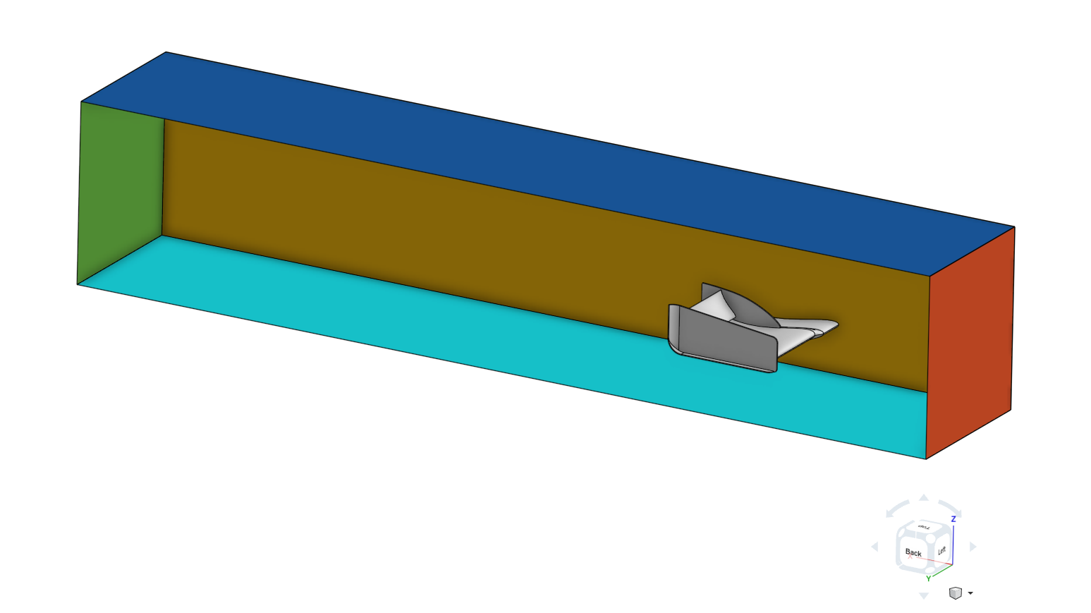
As a first simplification we can exploit the symmetry of the front wing. Simulating only half of the wing reduces the computational effort by defining the inner surrounding wall (brown) as a symmetry plane.
The body of the wing is a physical wall (grey), which means that it involves friction and should be defined as so-called “no-slip walls”.
The outer (not visible here) and upper surrounding walls (blue) are necessary to limit the size of the domain we want to simulate since we are not able to simulate an infinitely large domain. In reality, these walls do not exist and should not interact with the flow. A good approximation here is to assume this wall as frictionless or so-called “slip walls”.
There is no relative motion between the air and the floor since the car is in motion. Thus, we will apply a wall velocity on the lower surrounding wall (cyan).
The bounding face on the right-hand side (red) will be defined as an inlet with a constant flow velocity profile.
The bounding face on the left-hand side (green) will be defined as an outlet with a constant pressure.
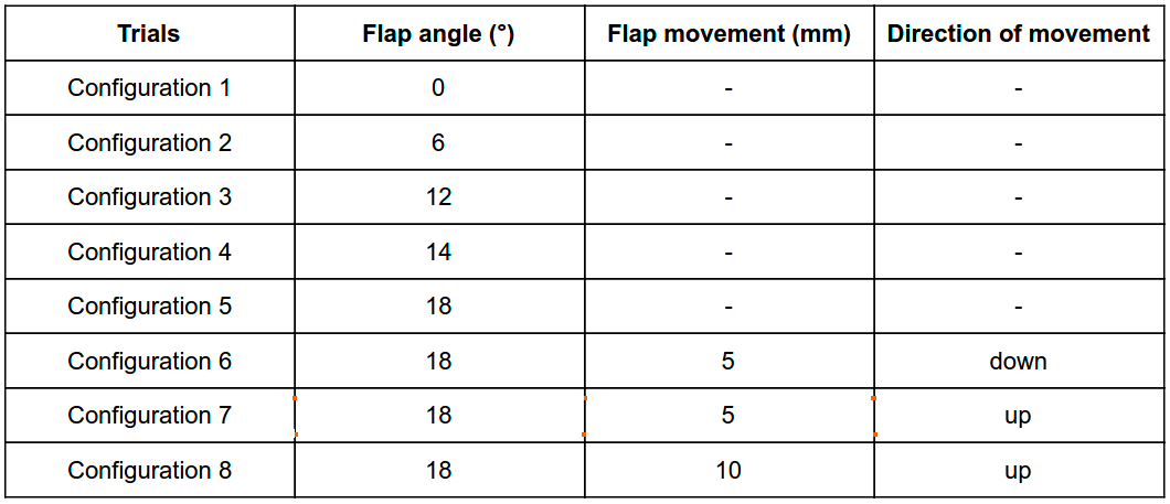
The different configurations which will be simulated in this exercise are shown in the table below:
Select 3 configurations for your own simulations. In order to conserve core hours it is not recommended to simulate all 8 configurations
First we will start with Configuration 1 and follow all the steps in detail. The other configurations will follow the same procedure and therefore will not be documented in detail.
To start this exercise, please import the project into your workspace by clicking on the link below:
Mesh Generation
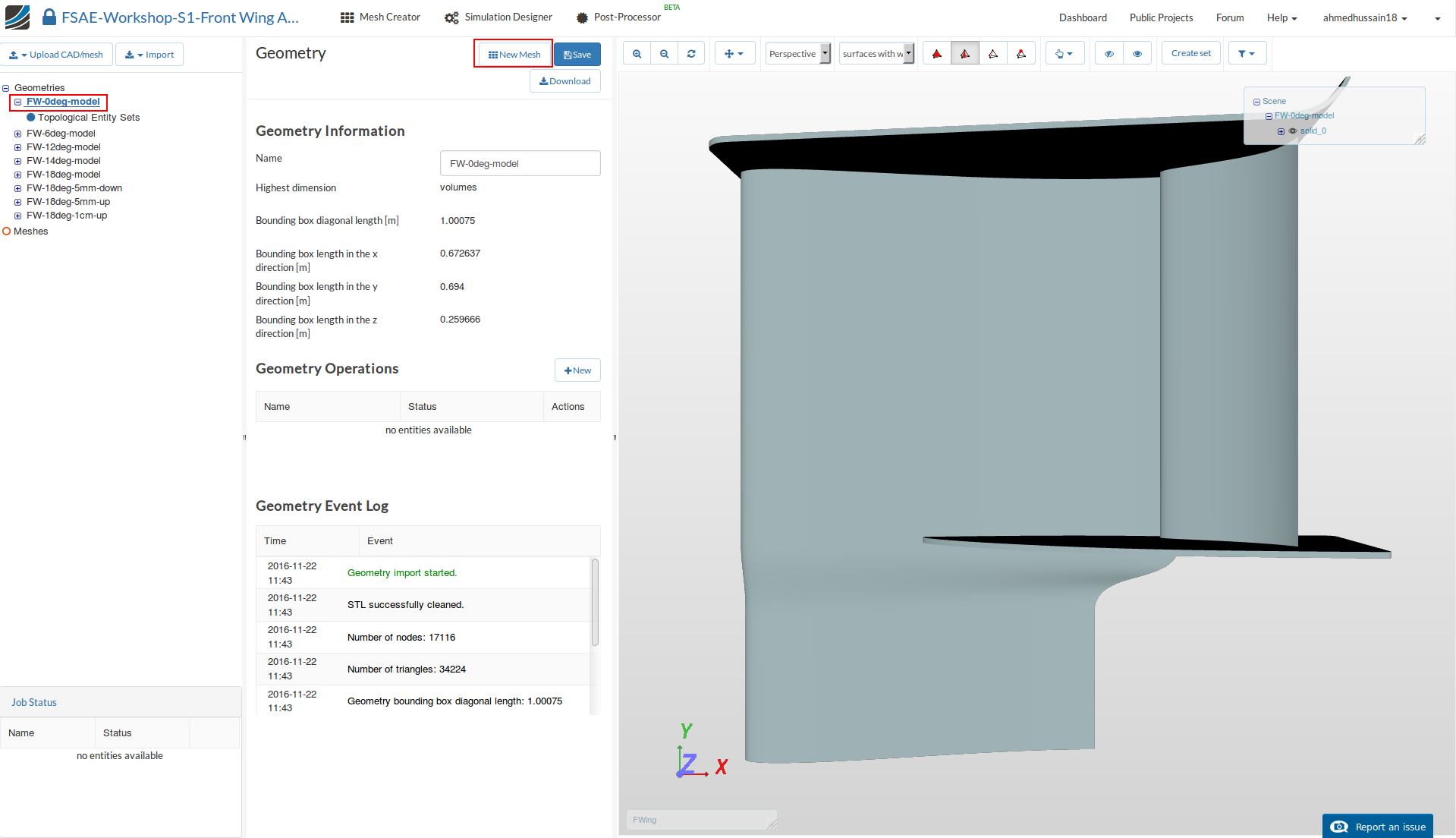
In the Mesh Creator tab, click on the geometry FW-0deg-model
Click the New Mesh button in order to start creating a new mesh on this geometry.
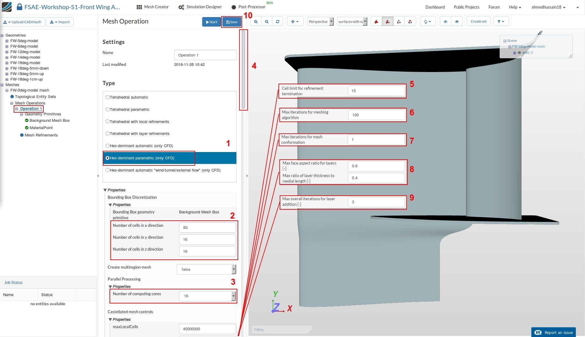
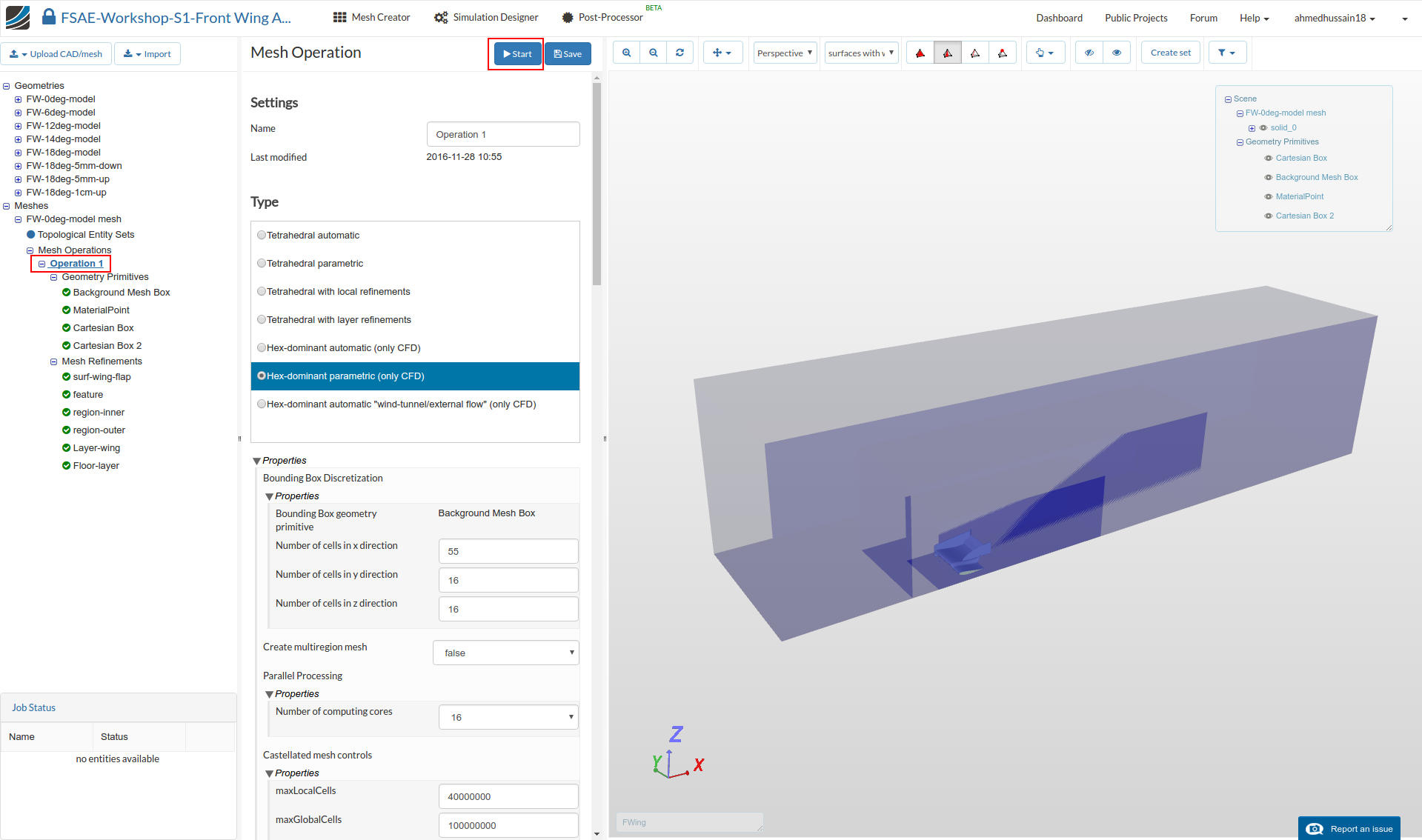
The new mesh operation will be generated automatically. Next change:
-
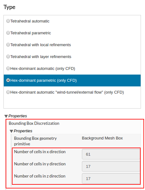
Set the Type to Hex-dominant parametric (only CFD).
-
Configure the Bounding Box geometry primitive to the following:
Number of cells in x direction to 60
Number of cells in y direction to 16
Number of cells in z direction to 16 -
Set the Number of parallel computing cores to 16
-
Scroll down to change other values to optimize the meshing parameters
-
Cell limit for refinement termination to 15
-
Max iterations for meshing algorithm to 100
-
Max iterations for mesh conformation to 1
-
Max face aspect ratio for layers and Max ratio of layer thickness to medial length to 0.6 and 0.4 respectively.
-
Max overall iterations for layer addition to 3
-
Click Save to register changes.
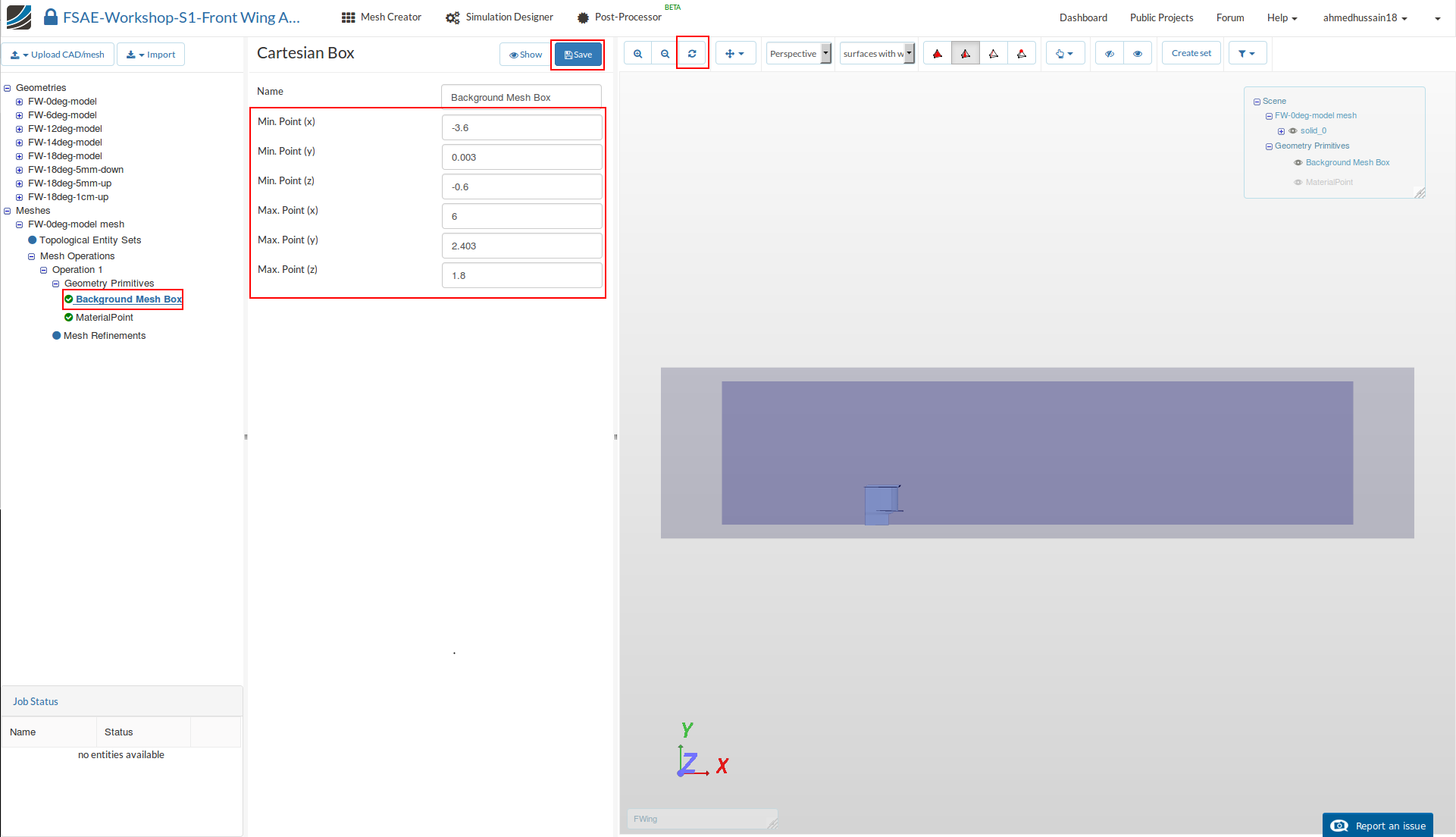
Background Mesh Box
Next go to the Background Mesh Box and change the Mesh Box dimensions to:
- Min. Point (x) = - 3.6
- Min. Point (y) = .003
- Min. Point (z) = - 0.6
- Max. Point (x) = 6
- Max. Point (y) = 2.403
- Max. Point (z) = 1.8
Click Save to save the changes. Click on the reset icon over the viewer to see the created mesh box in viewer.
Material Point
Go to the MaterialPoint and change the values to the following:
- center (x) = - 1.5
- center (y) = 0.5
- center (z) = - 0.5
Then click Save

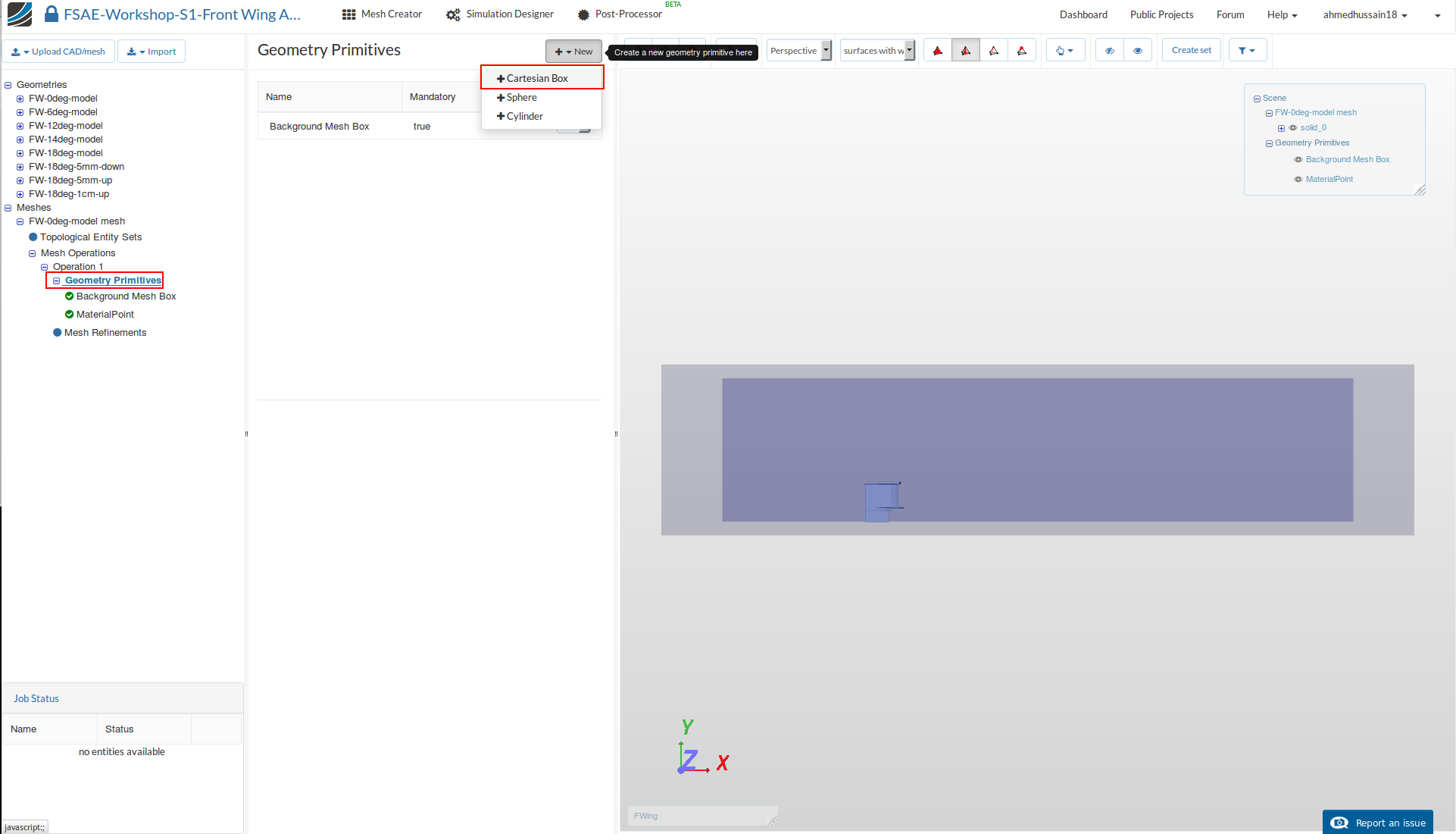
Cartesian Box
Next go back to the Geometry Primitives and click on + New and then Cartesian Box to define a new Cartesian Box that will be used to define a mesh refinement region.
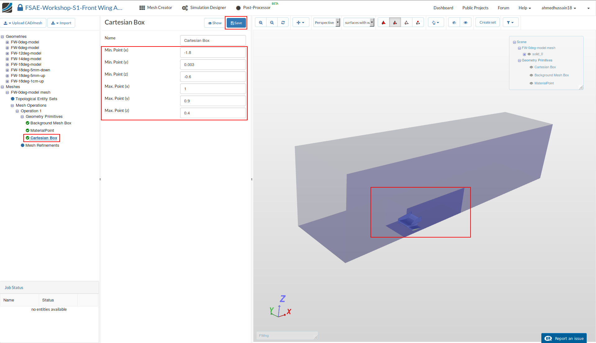
After creating a new Cartesian Box, you will be directed to the definition of this Cartesian Box. Change the dimensions of the box to the following:
- Min. Point (x) = - 1.8
- Min. Point (y) = .003
- Min. Point (z) = - 0.6
- Max. Point (x) = 1
- Max. Point (y) = 0.9
- Max. Point (z) = 0.4
Click Save to register your changes.
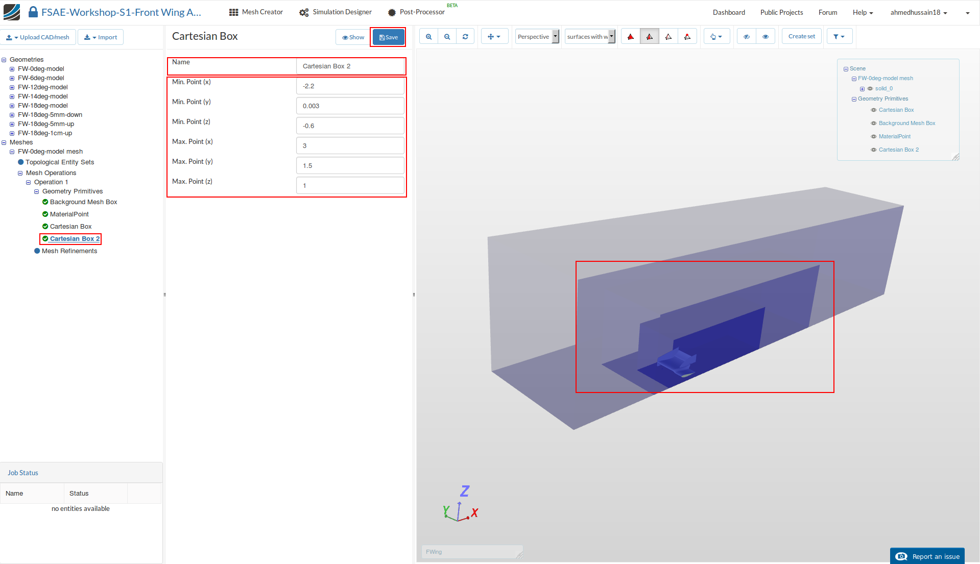
Cartesian Box 2
Follow the same procedure to define another Cartesian Box for further refinement definitions. Rename it to Cartesian Box 2. This time change the values to the following:
- Min. Point (x) = -2.2
- Min. Point (y) = .003
- Min. Point (z) = -0.6
- Max. Point (x) = 3
- Max. Point (y) = 1.5
- Max. Point (z) = 1
Click Save to register your changes
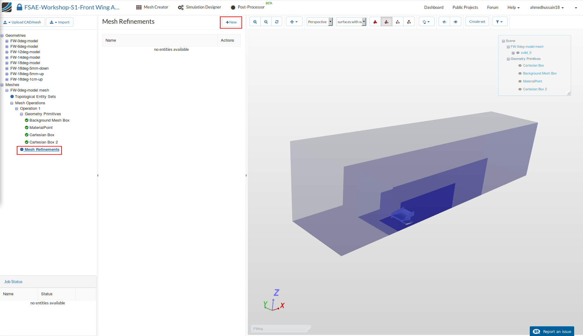
A good mesh requires well defined refinements. Now we will start creating the mesh refinements. For this proceed to Mesh Refinements and click +New
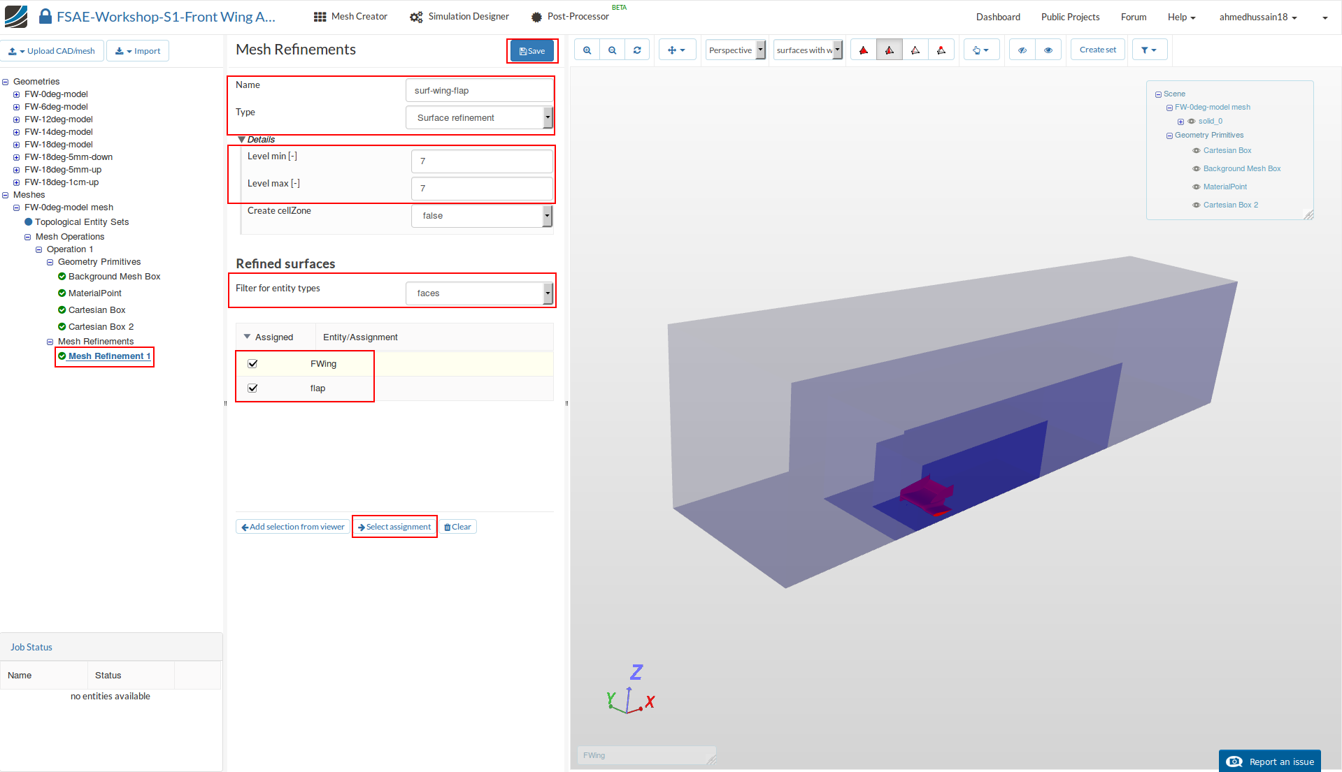
Mesh Refinement 1
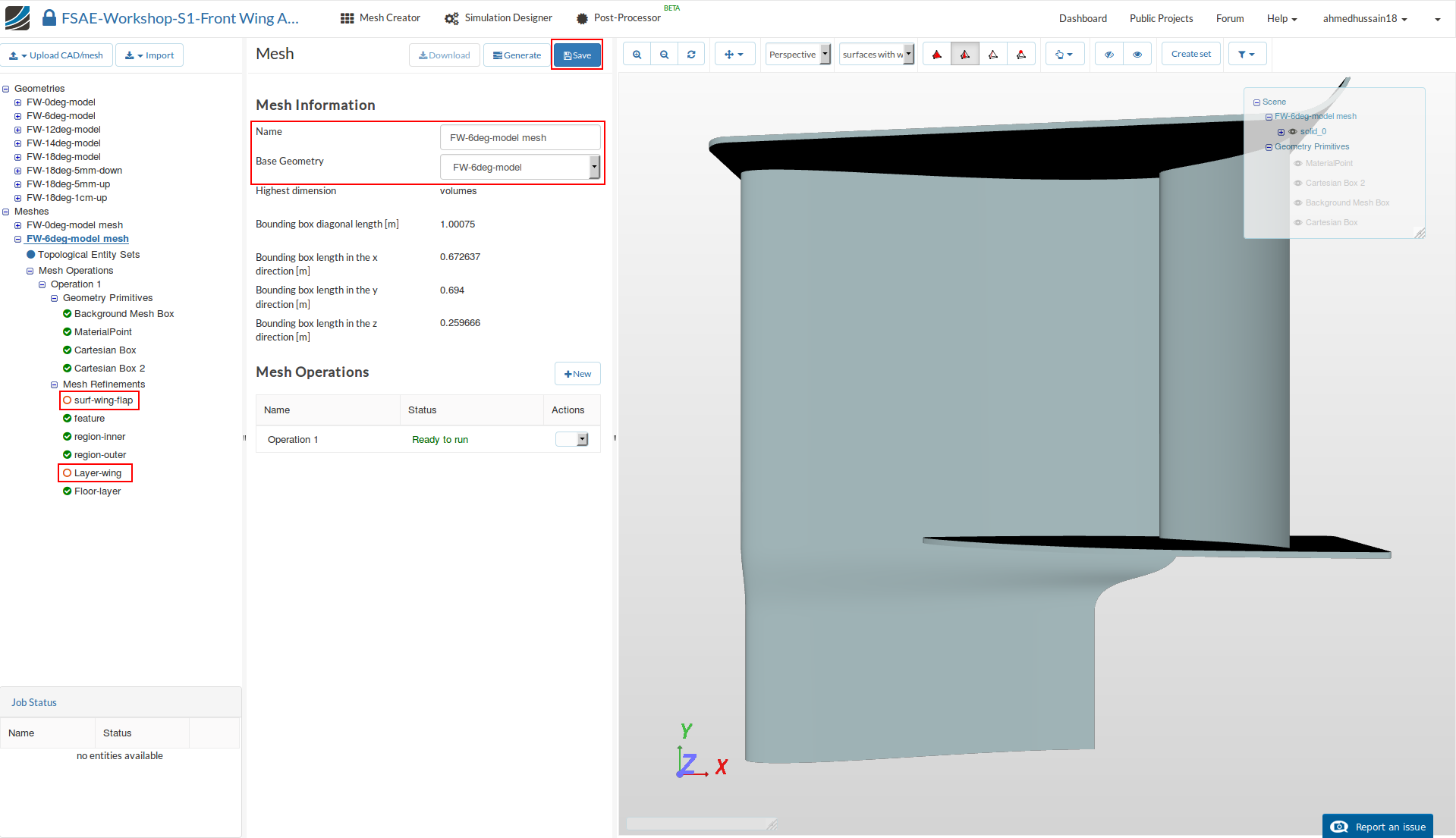
The new mesh refinement will be created. Rename it to surf-wing-flap (optional).
Change the Type to Surface refinement and then both Level min and Level max to 7 respectively.
Change the Filter for entity types to faces and select FWing and flap
Click Select assignment in order to see the selected assignment highlighted in the viewer.
Click Save to register your changes.
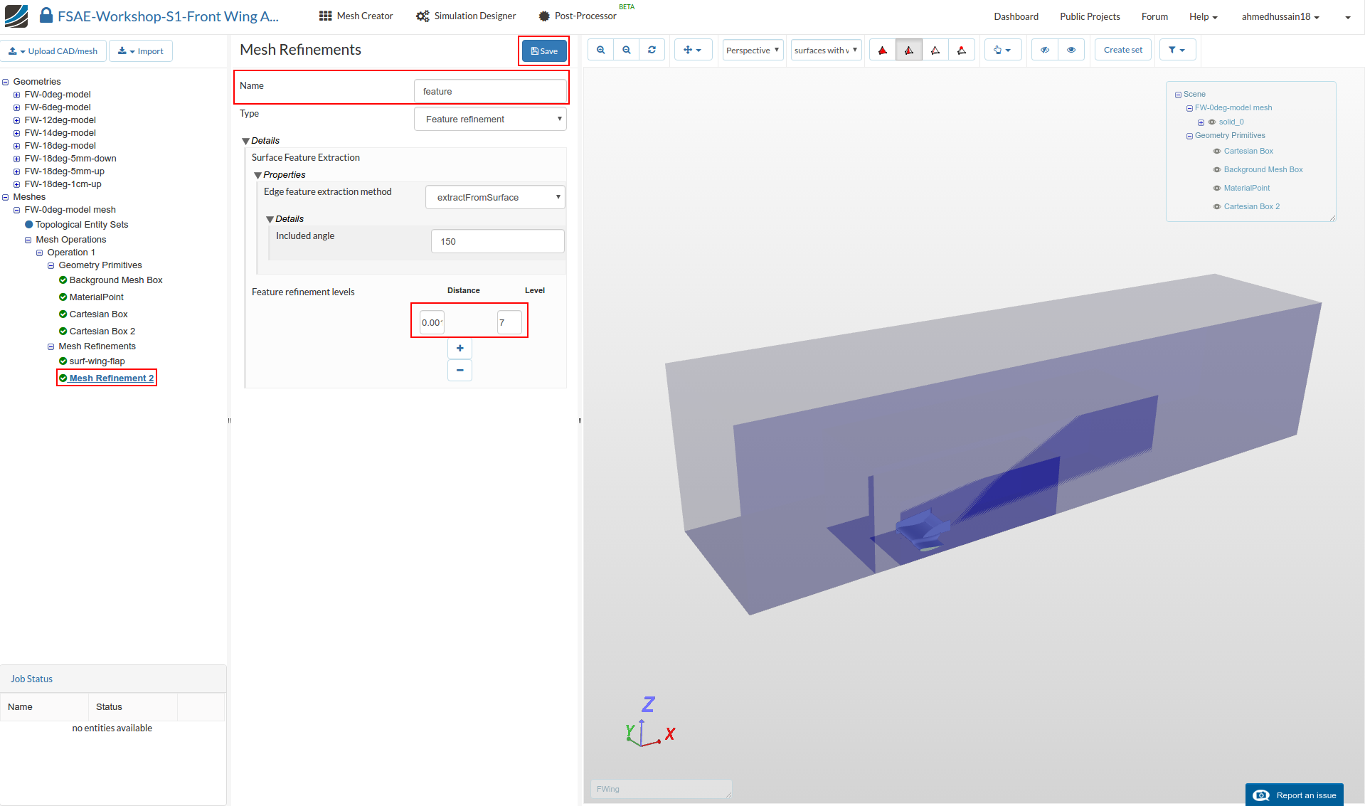
Mesh Refinement 2
Following the same procedure,create a new refinement and name it feature (optional).
Change Feature refinement levels Distance and Level to 0.001 and 7 respectively.
Then click Save
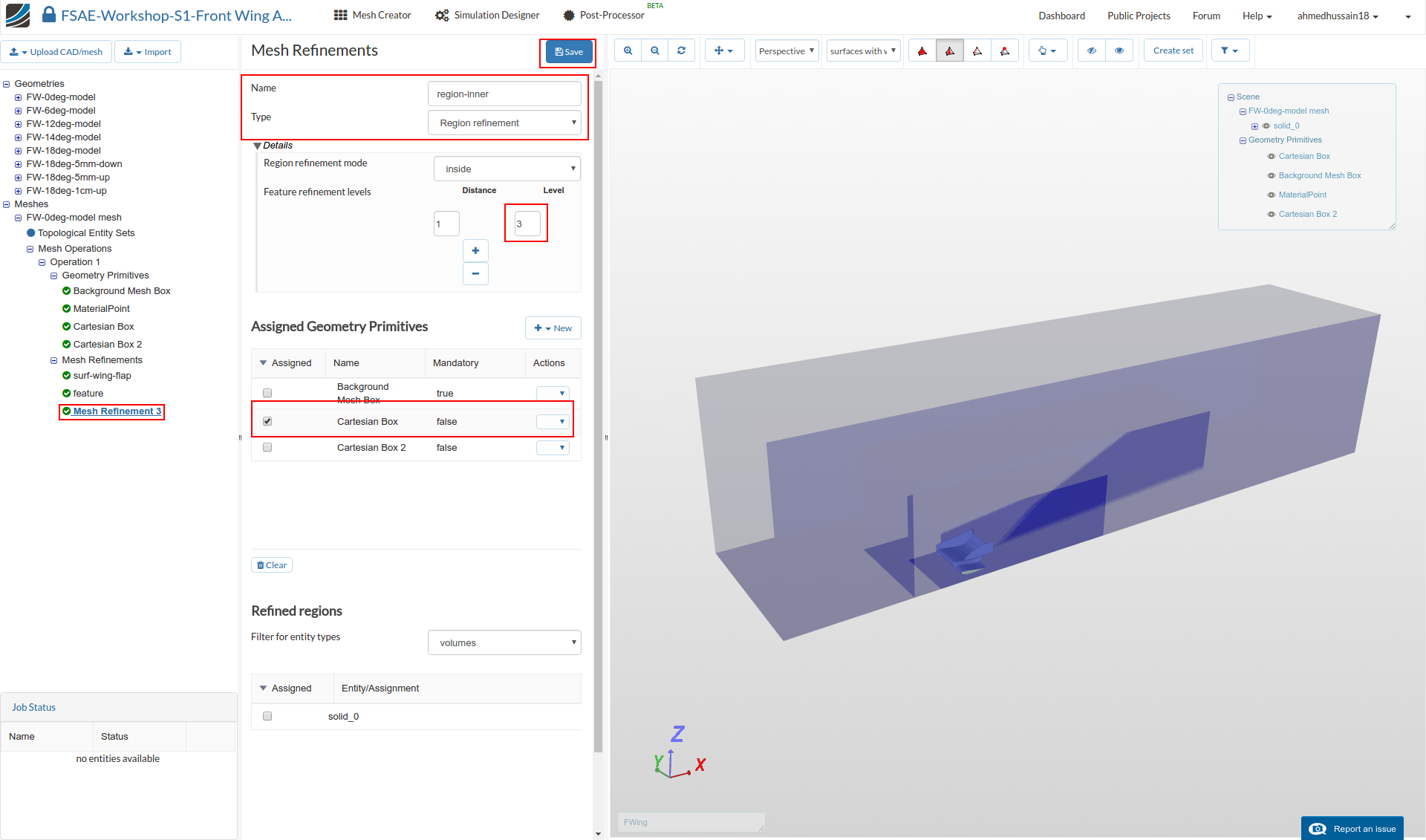
Mesh Refinement 3
In order to create a separate region refinement for the inner Cartesian Box, create a new refinement and rename it to region-inner (optional).
Change Type to Region refinement and then Feature refinement levels Level to 3
Select Cartesian Box under Assigned Geometry Primitives and click Save to register the refinements for this specific cartesian box.
Mesh Refinement 4
Create a new refinement for the other Cartesian Box. This time rename it to region-outer (optional).
Change Type to Region refinement and then and then Feature refinement levels Level to 1
Select Cartesian Box 2 under Assigned Geometry Primitives and click Save to register the refinements for this specific Cartesian Box.

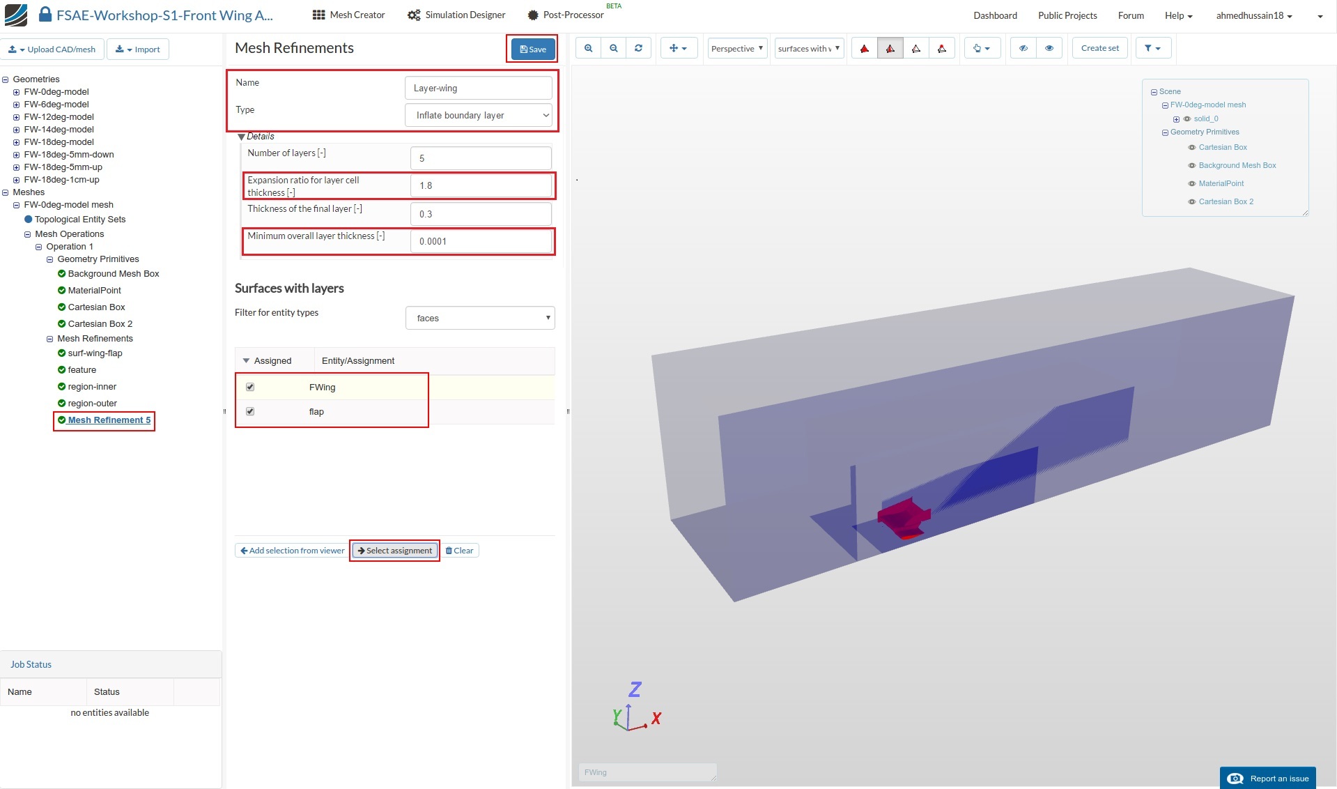
Mesh Refinement 5
Next we will define layers over the surfaces on the whole wing and the floor. Layers will allow us to capture the results more accurately within the areas we are interested in.
Create a new refinement and rename it to Layer-wing (optional).
Change Type to Inflate boundary layer and further change Expansion ratio for layer cell thickness [-] and Minimum overall layer thickness [-] to 1.8 and 0.0001 respectively.
Select FWing and flap under Surfaces with layers and click Select assignment in order to review the selected surfaces in the viewer.
Click Save to register your changes.
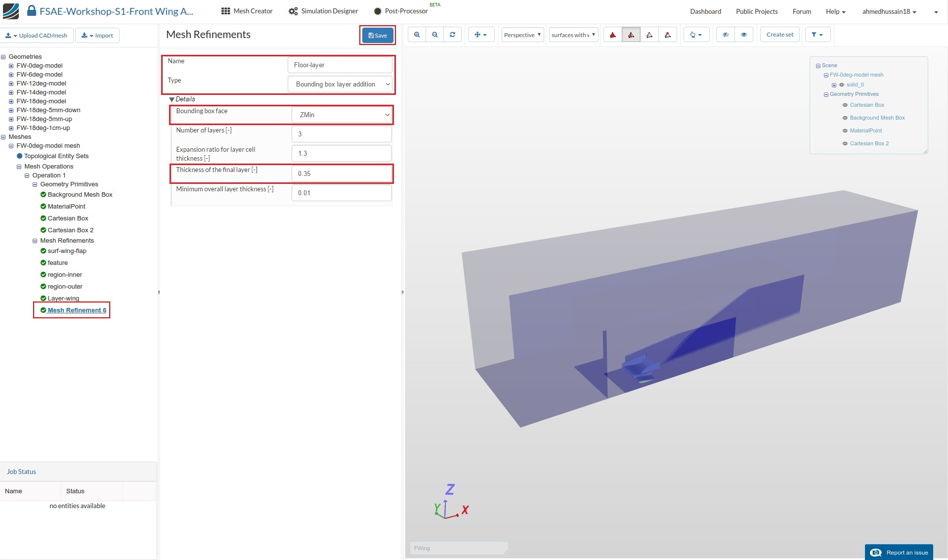
Mesh Refinement 6
For the floor layers, create a new refinement and rename it to Floor-layer (optional).
Change Type to Boundary box layer addition
Change Bounding box face to Zmin and then the Number of layers [-] and Thickness of the final layer [-] to 3 and 0.35 respectively.
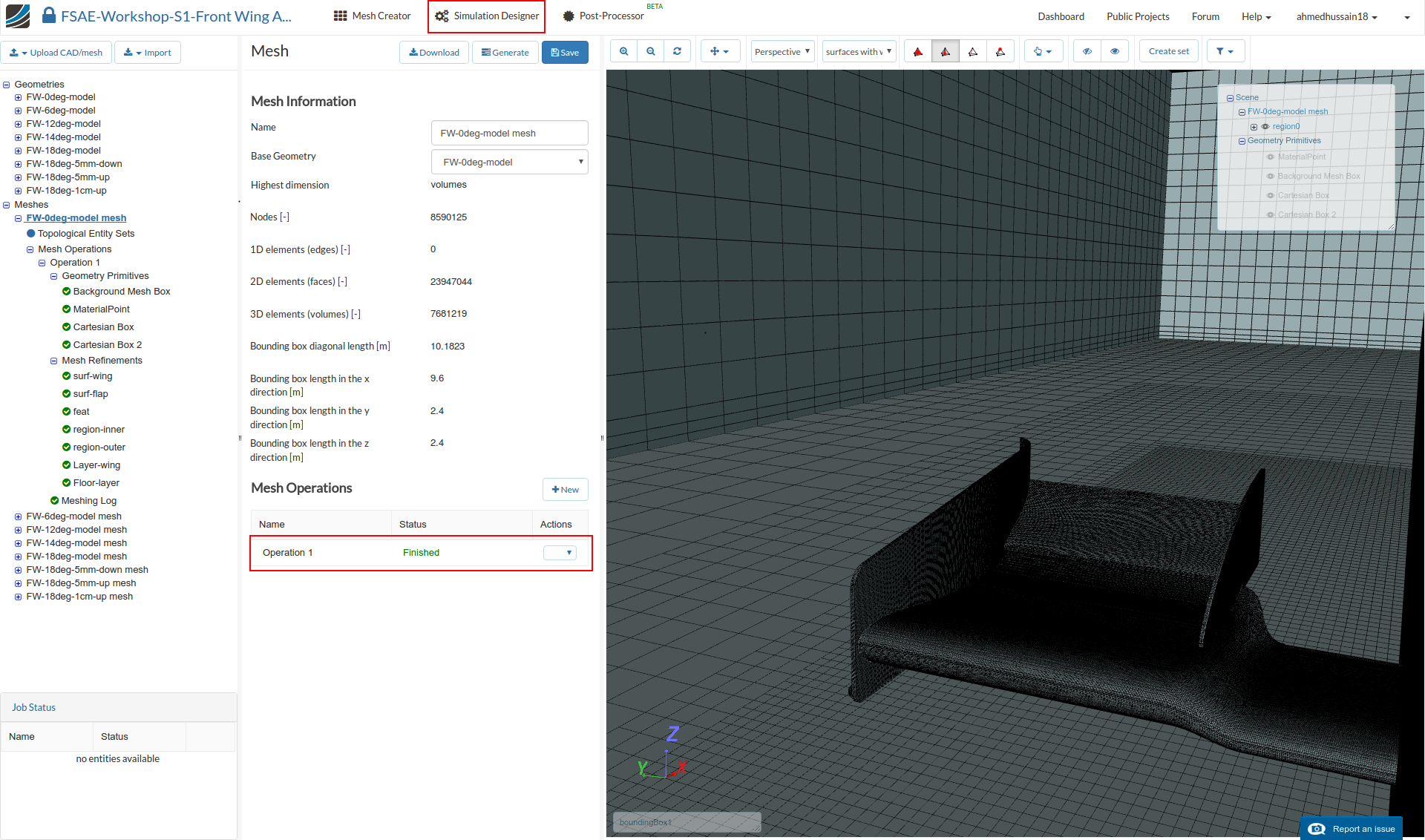
Once you have defined all of the mesh refinements, go back to the Operation 1 and click Start in order to submit the meshing job to the server. Due to the fineness of the mesh, the meshing could take 15 to 20 minutes to finish.
Additional Meshes
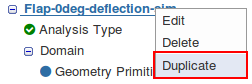
While the first mesh job is running, take advantage of the parallel computing and proceed to start setting up all the other configurations. You don’t have to perform all the meshing operations again from scratch. Just duplicate the already created mesh by right clicking on it and then click Duplicate.
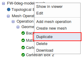
Rename the duplicated mesh to FW-XXdeg-model mesh (where XX is the flap degrees) and use the dropdown to change the Base Geometry to the model with the corresponding angle. Then click Save. Now you will have to reassign the Fwing and flap faces for surf-wing-flap and Layer-wing refinements and start the meshing operation.
Once the meshing of the first geometry i.e. FW-0deg-model is finished, you can proceed to Simulation Designer without waiting for others to complete in order to set up the simulation in parallel.
Simulation Setup
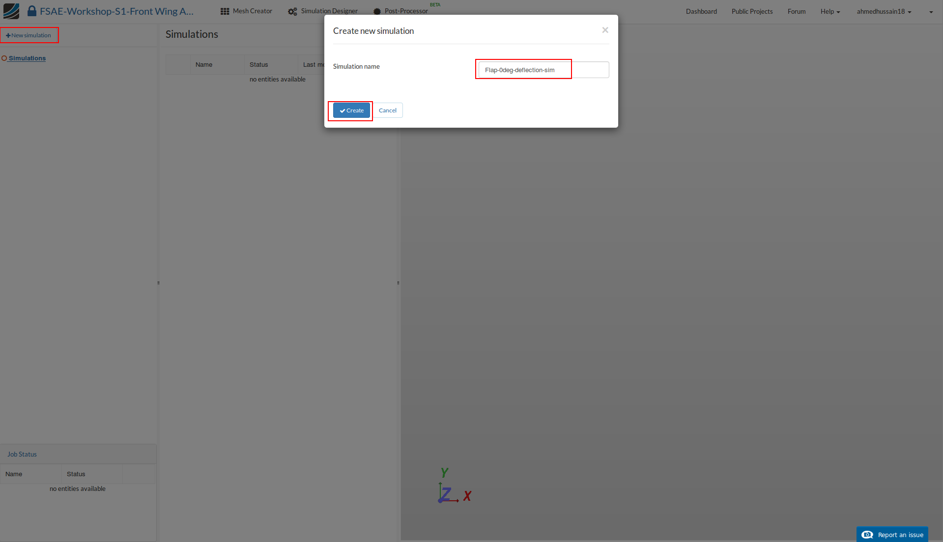
Once you are in Simulation Designer, click New Simulation in order to start setting up the simulation. A new simulation creating window will pop up. Rename it to Flap-0deg-deflection-sim (optional) and click Create in order to create a new simulation.
Analysis type
In Analysis Type, switch to Fluid dynamics and then select Incompressible. You don’t have to change any properties here.
Click Save to select this analysis type.
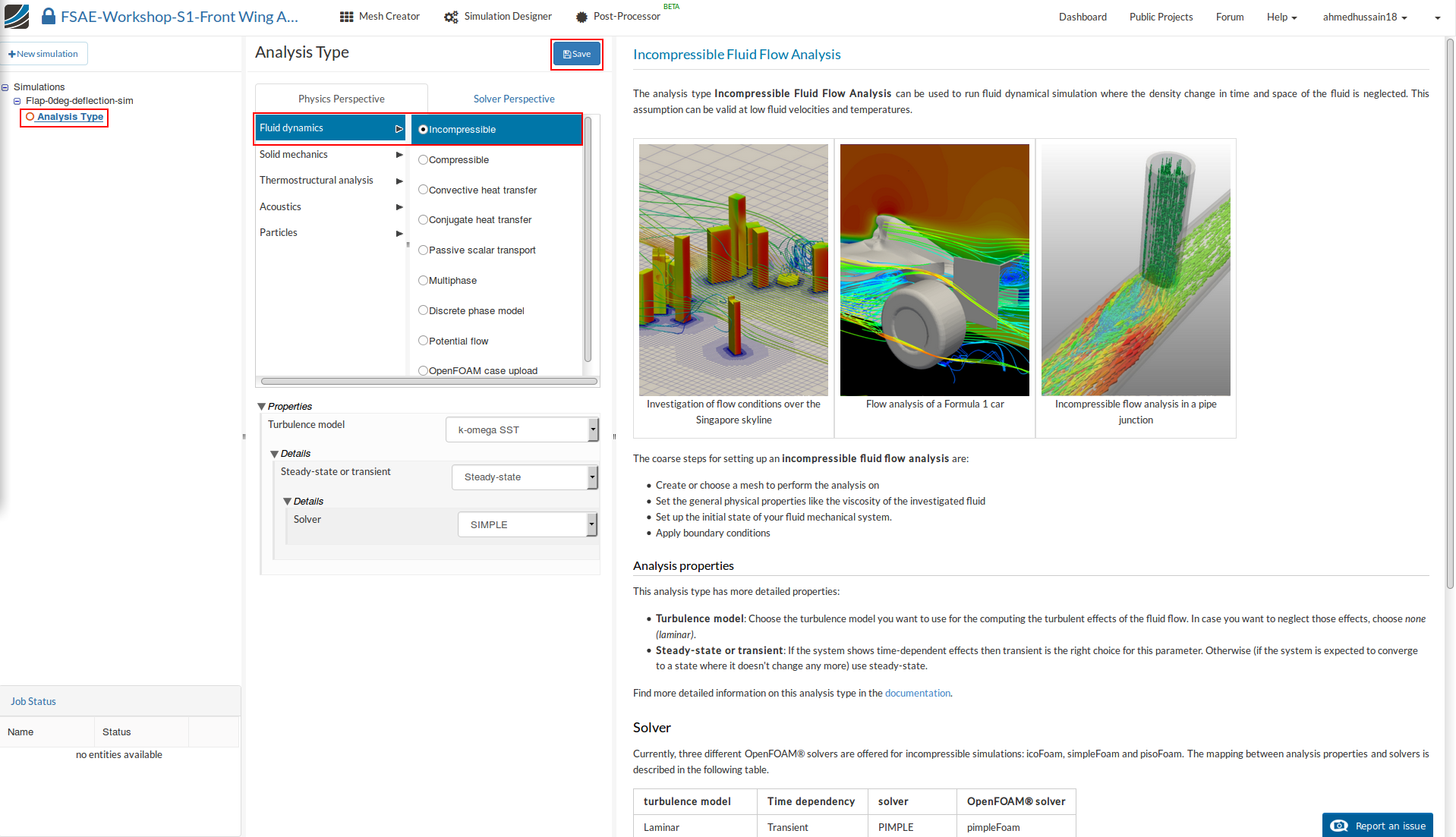
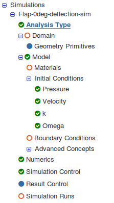
Once you save the analysis type, you will see the expanded tree. All the red entities shows that they must be set up in order to perform a successful simulation run.
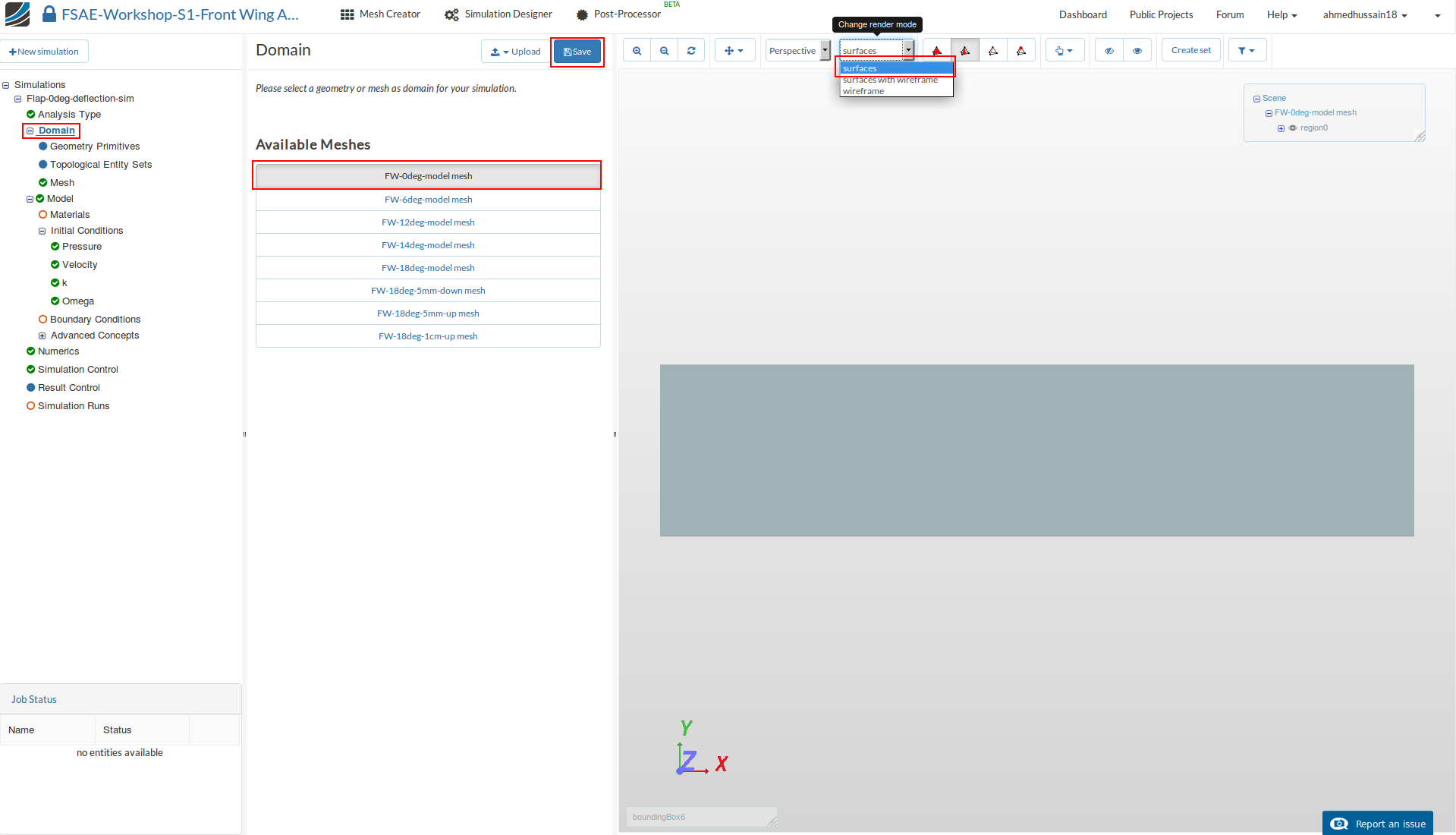
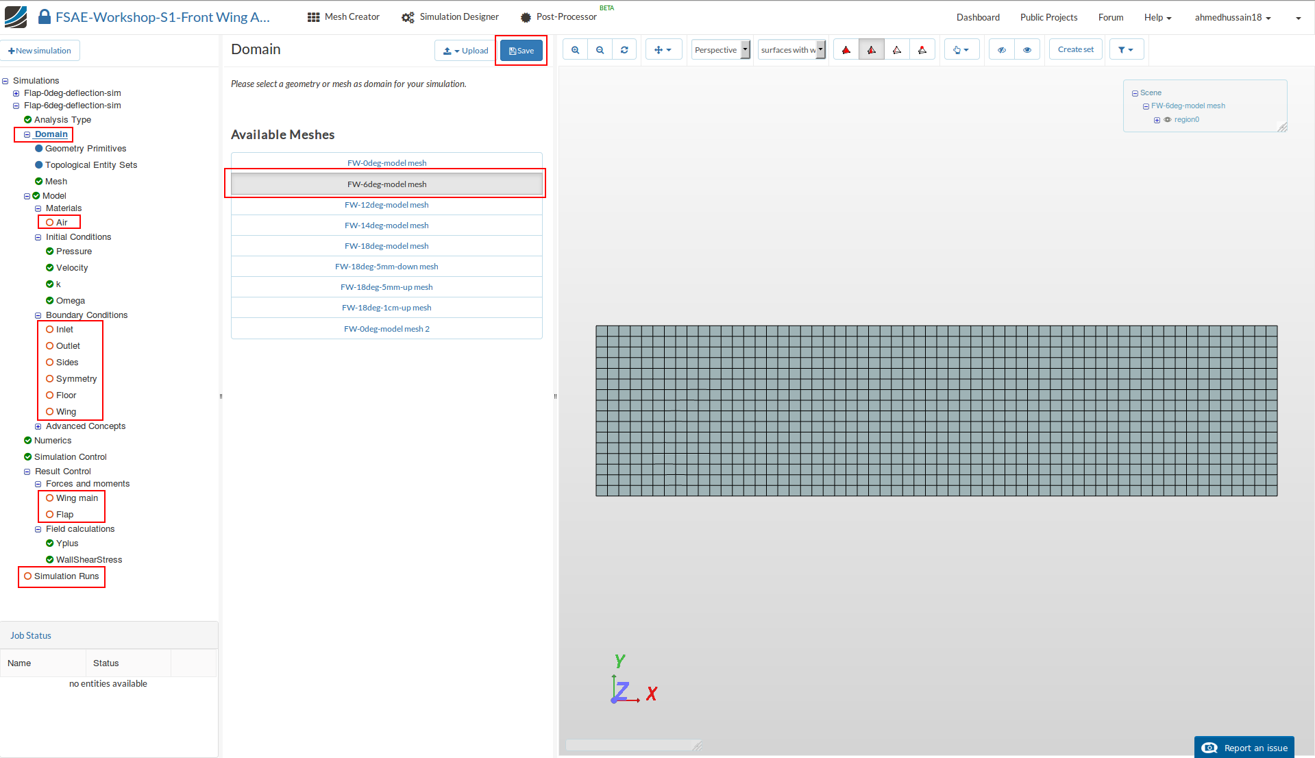
Domain
Next you have to select a domain on which this simulation will be performed. Proceed to Domain and select FW-0deg-model mesh and click Save.
After a while you will see the loaded mesh of the selected domain in the viewer. For the easier mesh handling, it is recommended to switch to the surfaces render mode in the top viewer bar.
Material
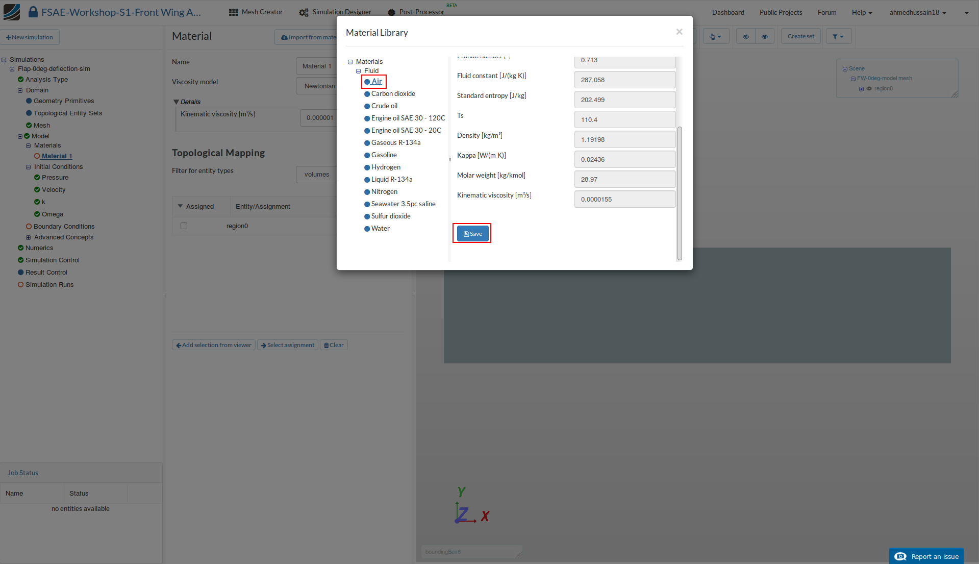
Next we have to define the fluid material. Go to Materials and click on +New to create a new material.
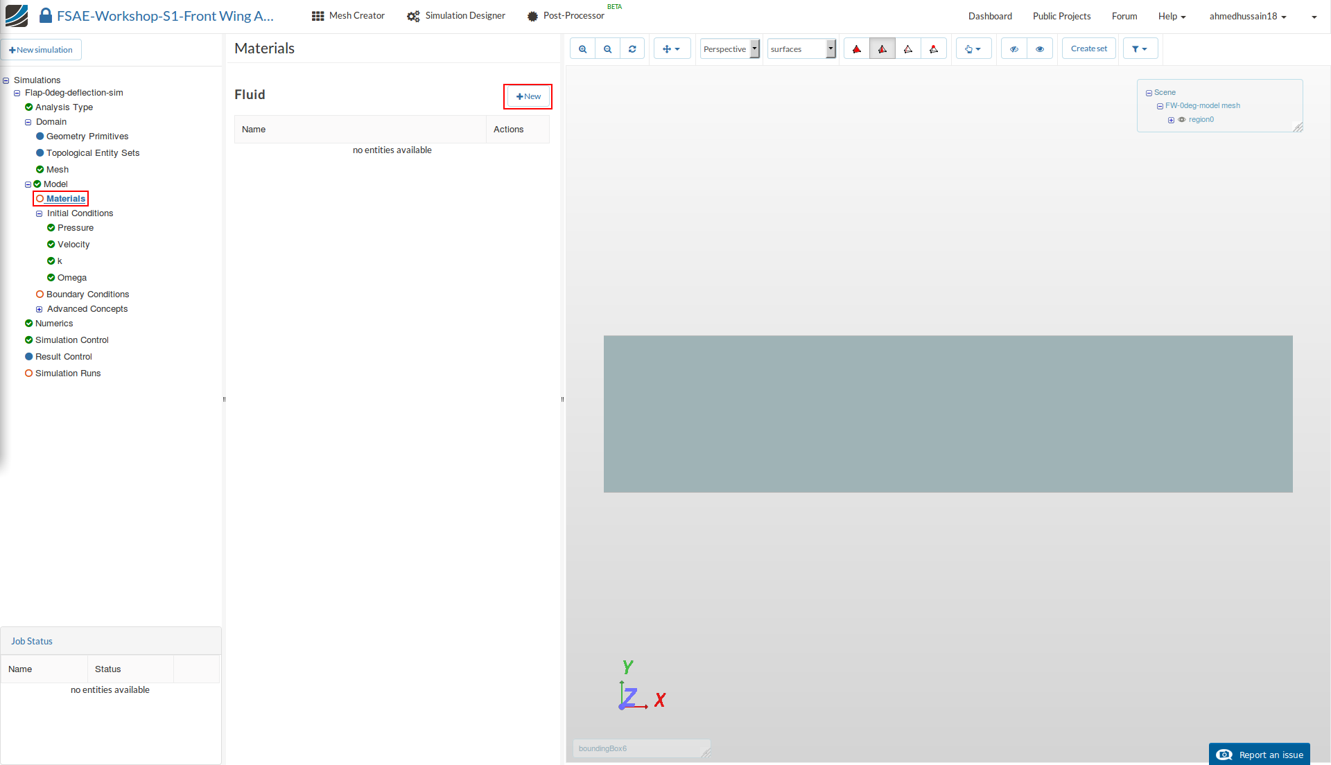
Click on Import from material library to import the desired material from the material database.
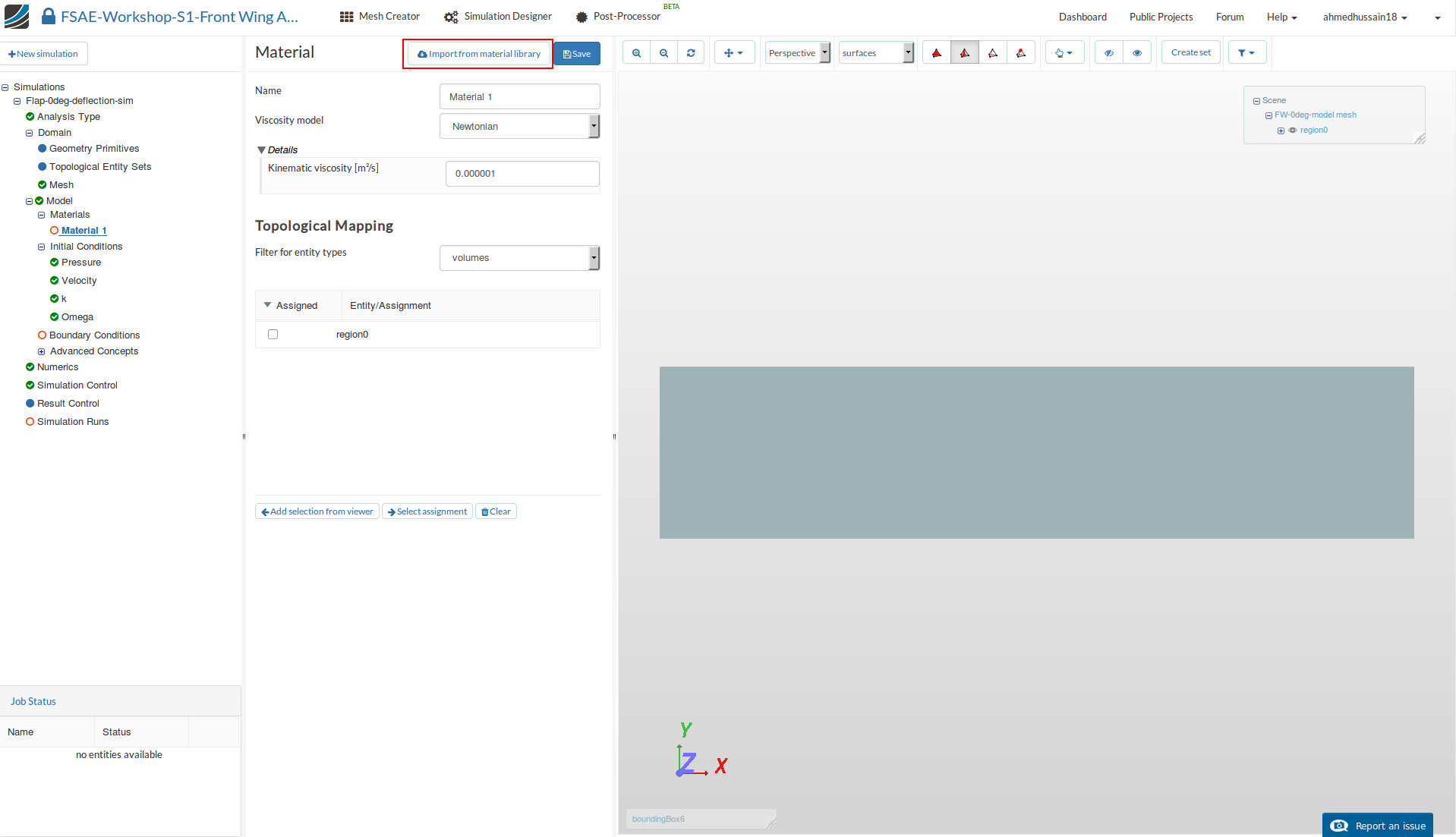
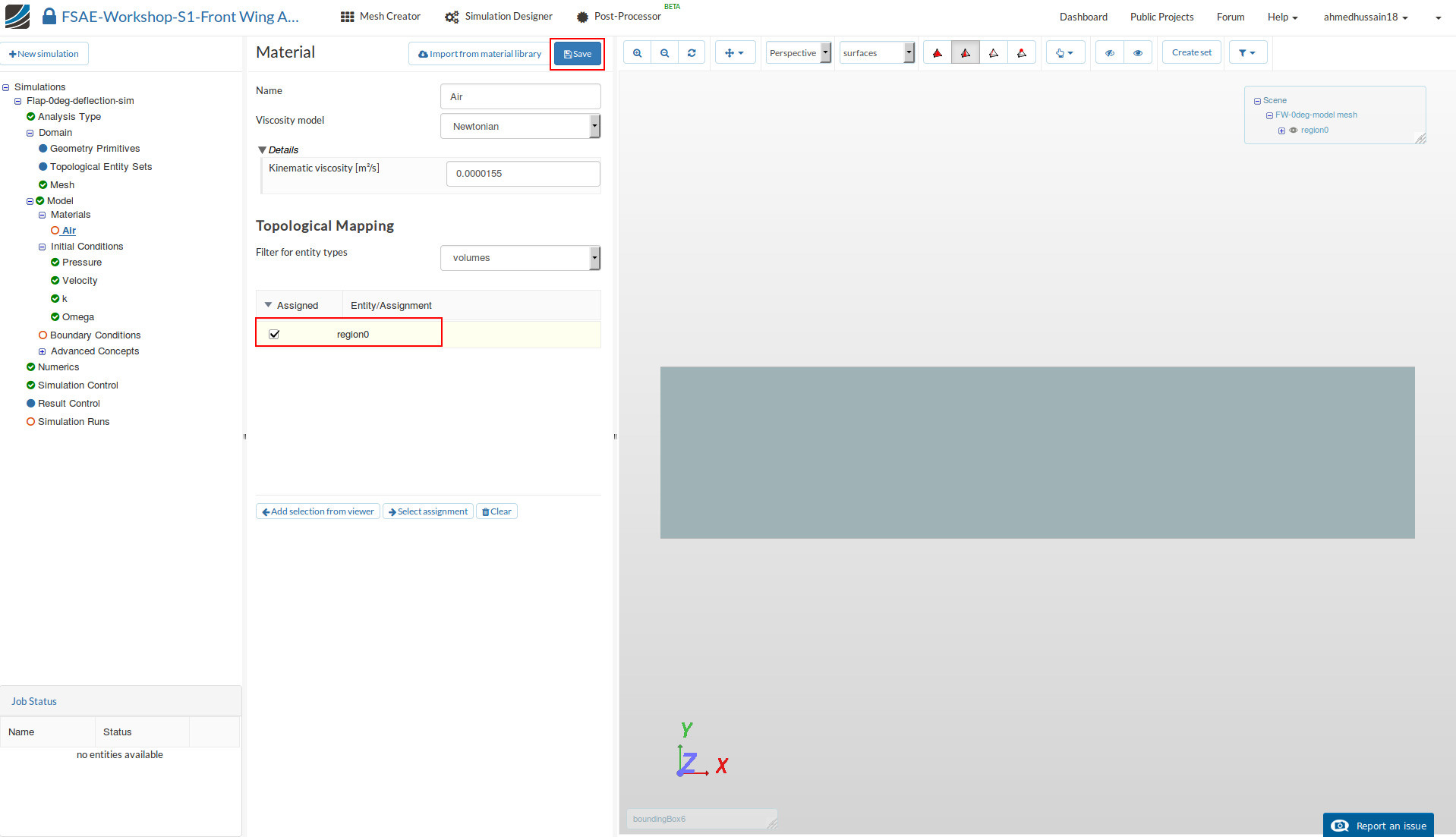
Select Air and click Save to import this material directly from the library.
Select region0 under Topological Mapping and then click Save in order to define the material for this region.
Initial Conditions
We will now proceed to change the initial conditions. Go to k and change the Turbulent kinetic energy value [m²/s²] value to 0.24 and click Save

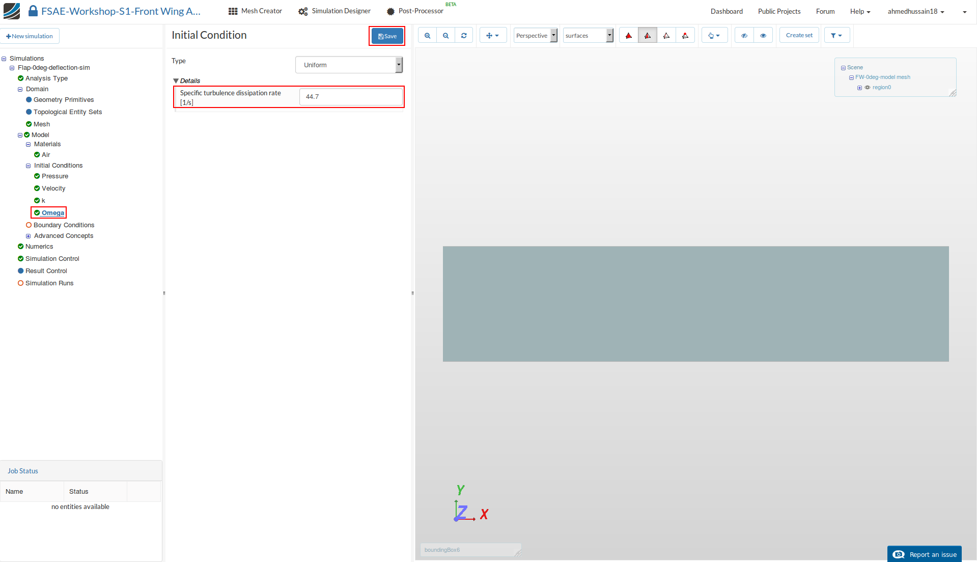
Next go to Omega and change Specific turbulence dissipation rate [1/s] to 44.7 and click Save
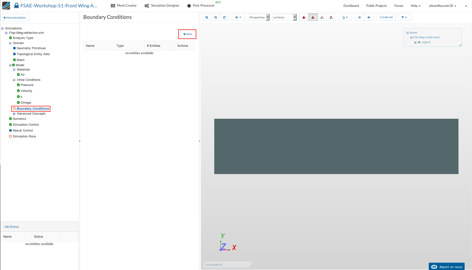
Boundary Conditions
Now we will proceed to the most crucial and important section of the simulation setup. We will define one by one the inlet and outlet boundary conditions. We will then define the boundary condition for the sides, symmetry, floor and wing.
Go to Boundary Conditions and click +New in order to create a new boundary condition.
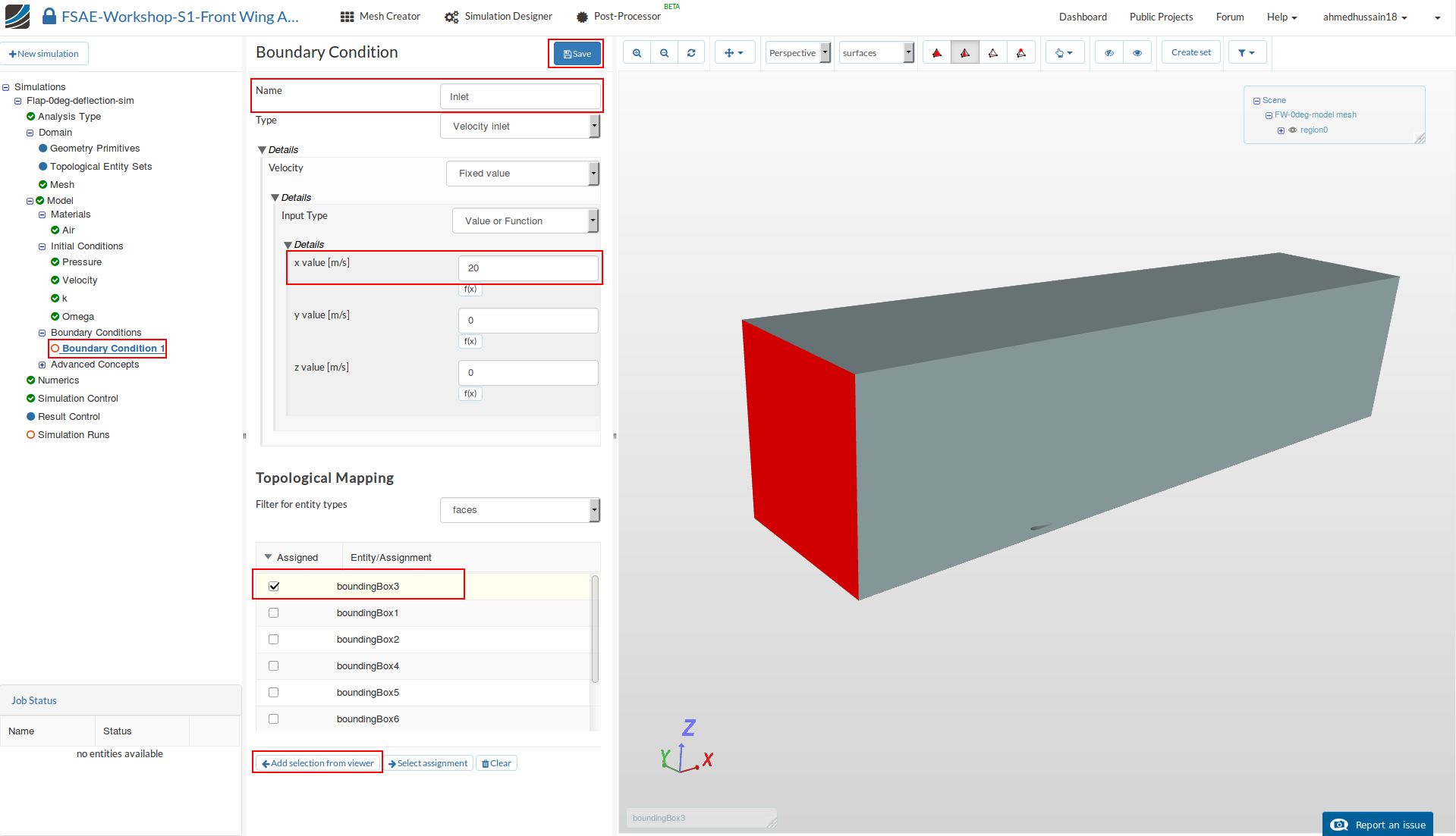
Inlet
Rename the newly created boundary condition to Inlet (optional).
Change the x value [m/s] of Velocity to 20
Select the front surface of the domain from the viewer and click on Add selection from viewer. This will add the selected surface under Topological Mapping i.e. boundingBox3 in this case.
Click Save to define the inlet boundary condition.
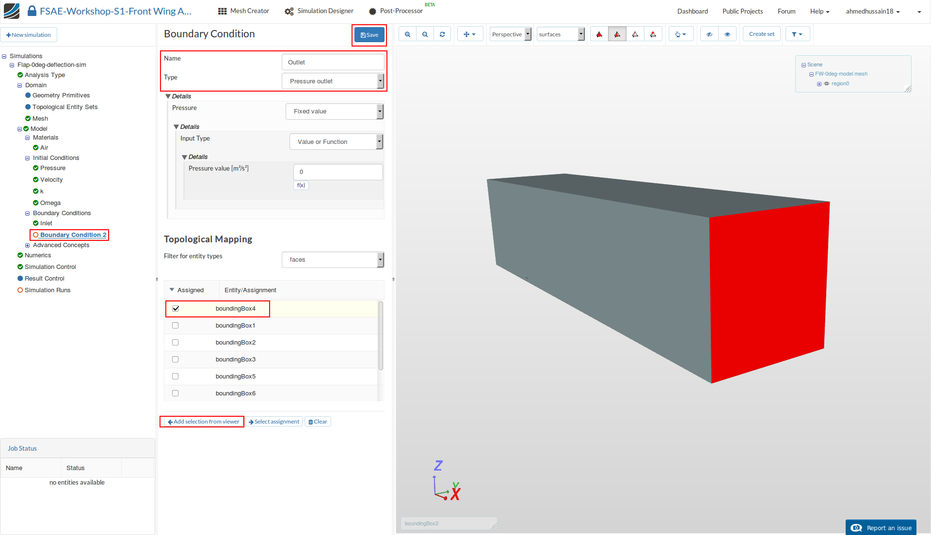
Outlet
Create a new Boundary Condition and name it Outlet (optional).
Change Type to Pressure Outlet and select the back surface of the domain and click on Add selection from viewer. This will add the selected surface under Topological Mapping i.e. boundingBox4 in this case.
Click Save to define the outlet boundary condition.
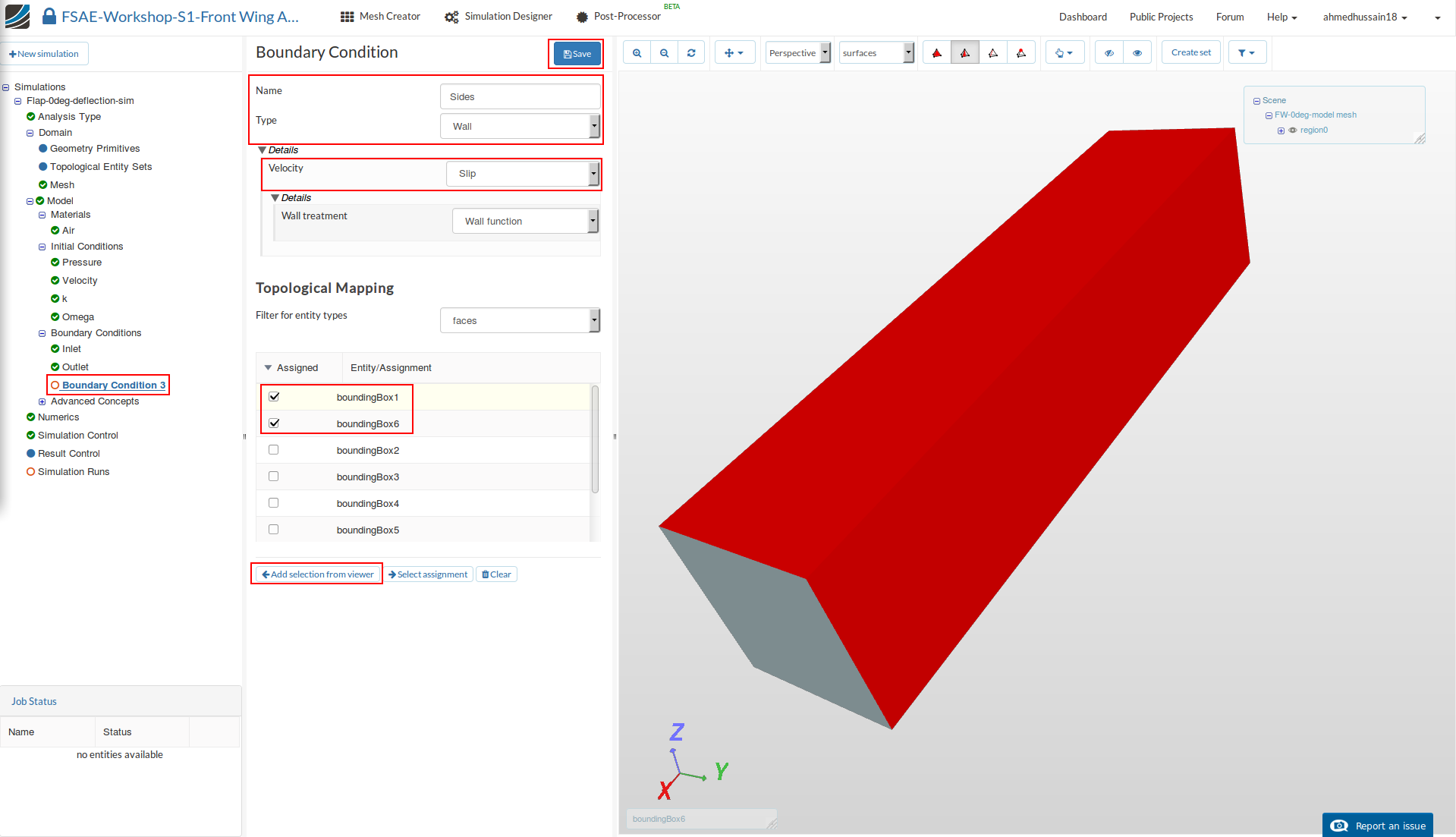
Sides
Create a new Boundary Condition and name it Sides (optional).
Change Type to Wall and Velocity to Slip.
Next select the two side surfaces of the domain and click on Add selection from viewer. This will add the selected surfaces under Topological Mapping i.e. boundingBox1 and boundingBox6 in this case.
- Click Save to define the boundary condition for the sides.
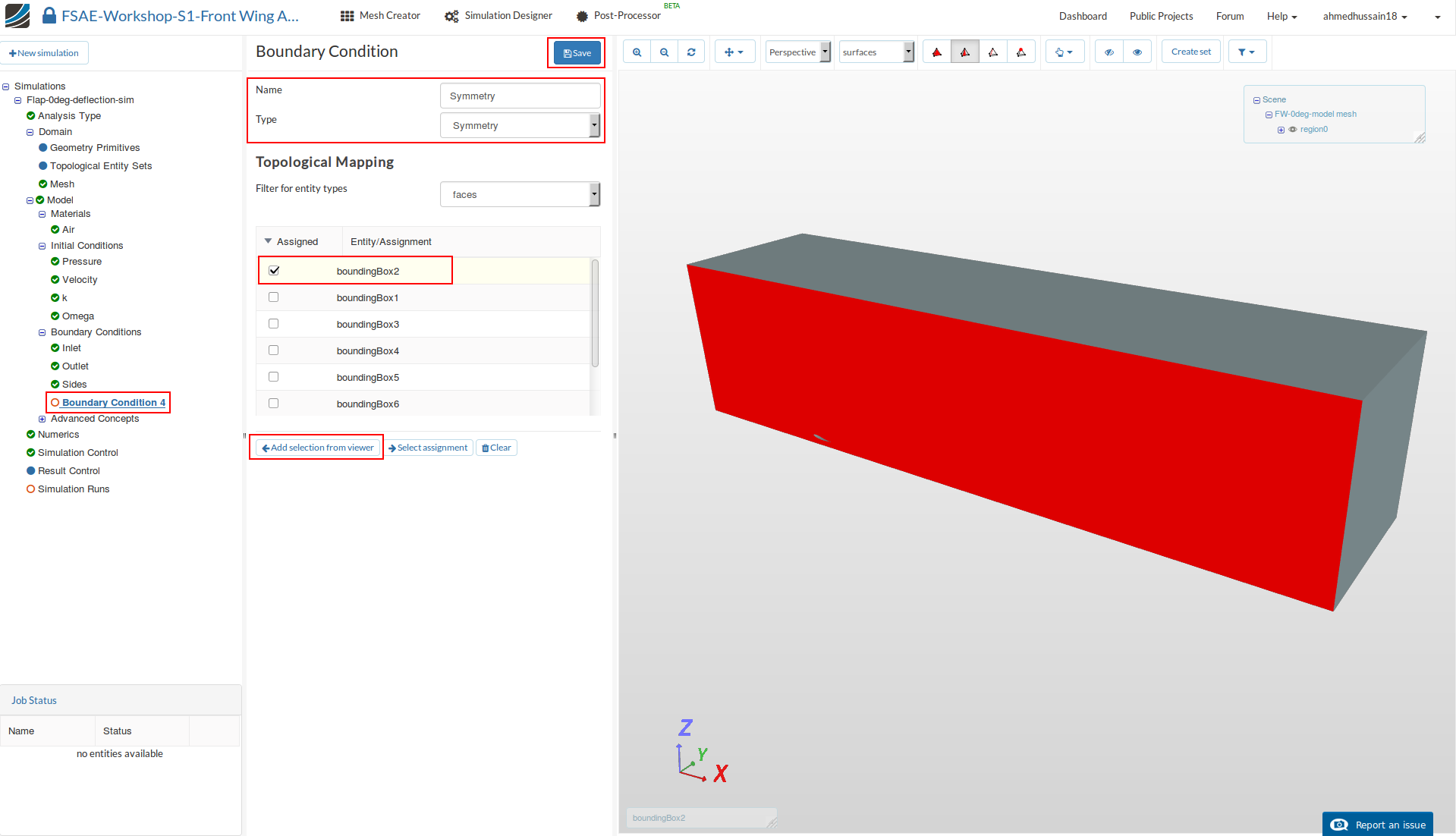
Symmetry
Next we will define the symmetry condition. Create a new Boundary Condition and name it Symmetry (optional).
Change Type and select the surface along symmetry of the domain and click on Add selection from viewer. This will add the selected surface under Topological Mapping i.e. boundingBox2 in this case.
Click Save to define the symmetry boundary condition.
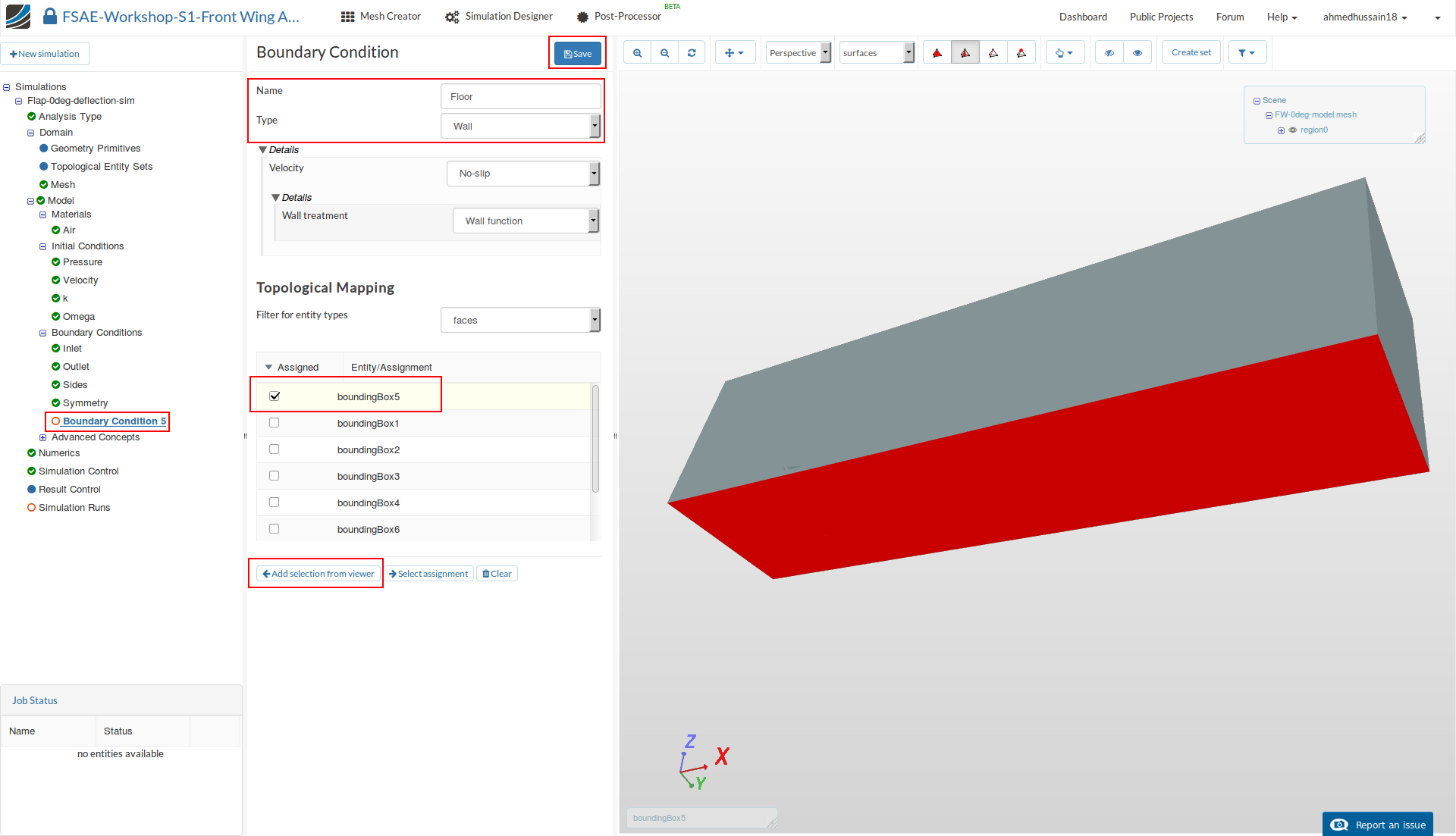
Floor
Create a new boundary condition and rename it to Floor (optional).
Change Type to Wall and select the lower surface of the domain and click on Add selection from viewer. This will add the selected surfaces under Topological Mapping i.e. boundingBox5 in this case.
Click Save to define the floor boundary condition.
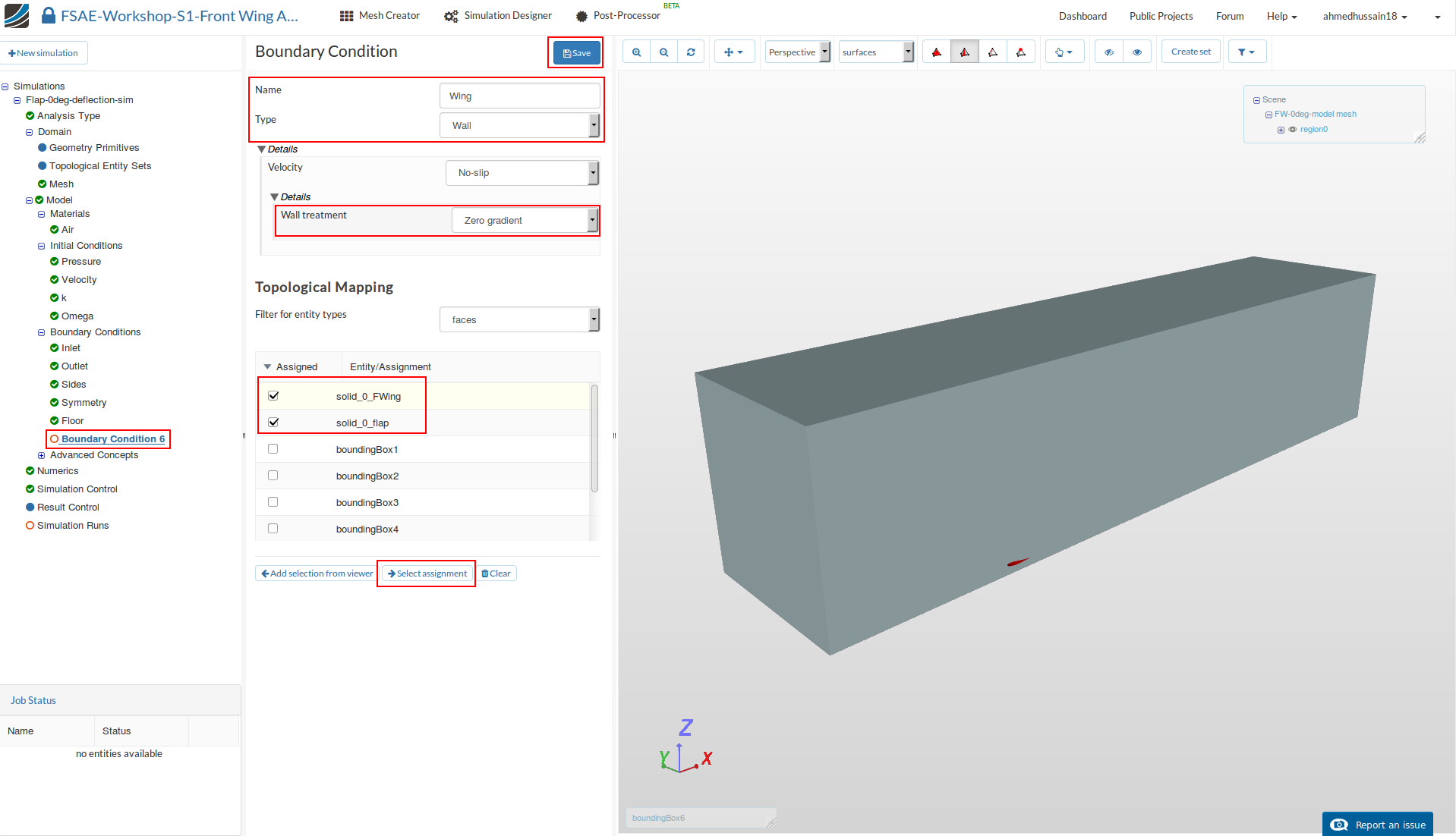
Wing
Lastly, we will define the boundary condition for the wing. Create a new boundary condition and rename it to Wing (optional).
Change Type to Wall and Wall treatment to Zero gradient.
Select solid_0_FWing and solid_0_flap under Topological Mapping and click Select assignment to see the selection in the viewer.
Click Save to define the boundary condition for the wing.
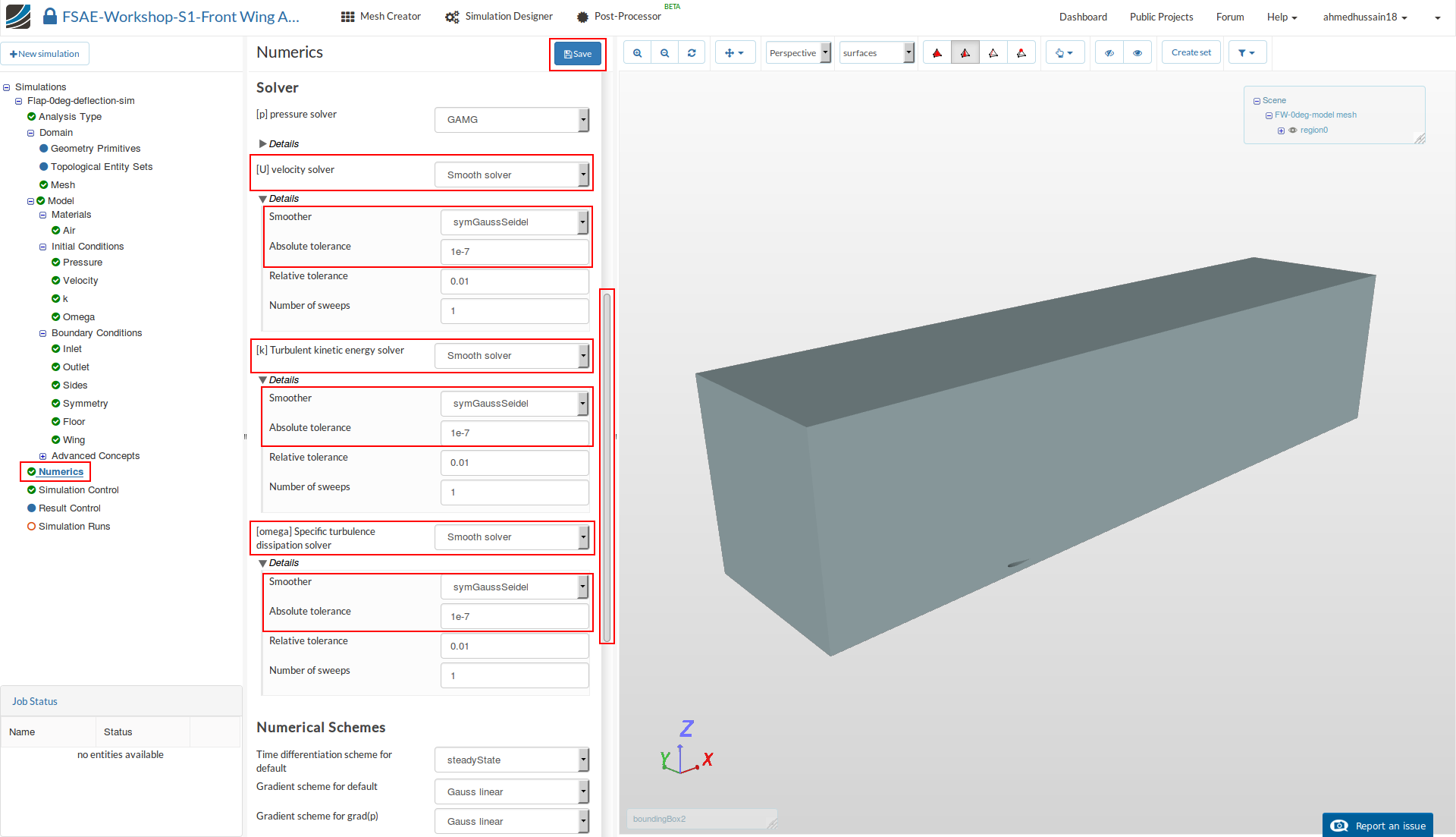
Numerics
After defining all the boundary conditions, we will proceed to set up the numerics for our simulation. Go to Numerics and scroll down until you reach Solver.
Under Solver, change [U] velocity solver to Smooth solver. Expand Details and change Smoother to symGaussSeidel and Absolute tolerance to 1e-7.
Do similar changes for [k] Turbulent kinetic energy solver and [omega] Specific turbulence dissipation solver.
Click Save to register your changes.
Simulation Control
Next we will define the our simulation interval and steps that needs to be recorded. Go to Simulation Control and change End time value [s] to 1500.
Expand Details under Write control and change Write interval (simulation time steps) to 1500.
Next change Number of computing cores and Maximum runtime [s] to 32 and 120000 respectively. The Maximum runtime [s] is set too high just to be on a safe side.
Click Save to register your changes.

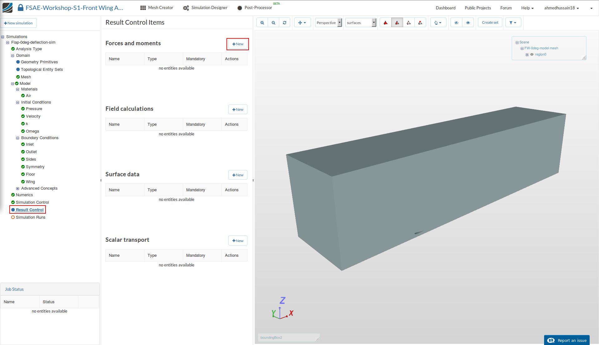
Result Control
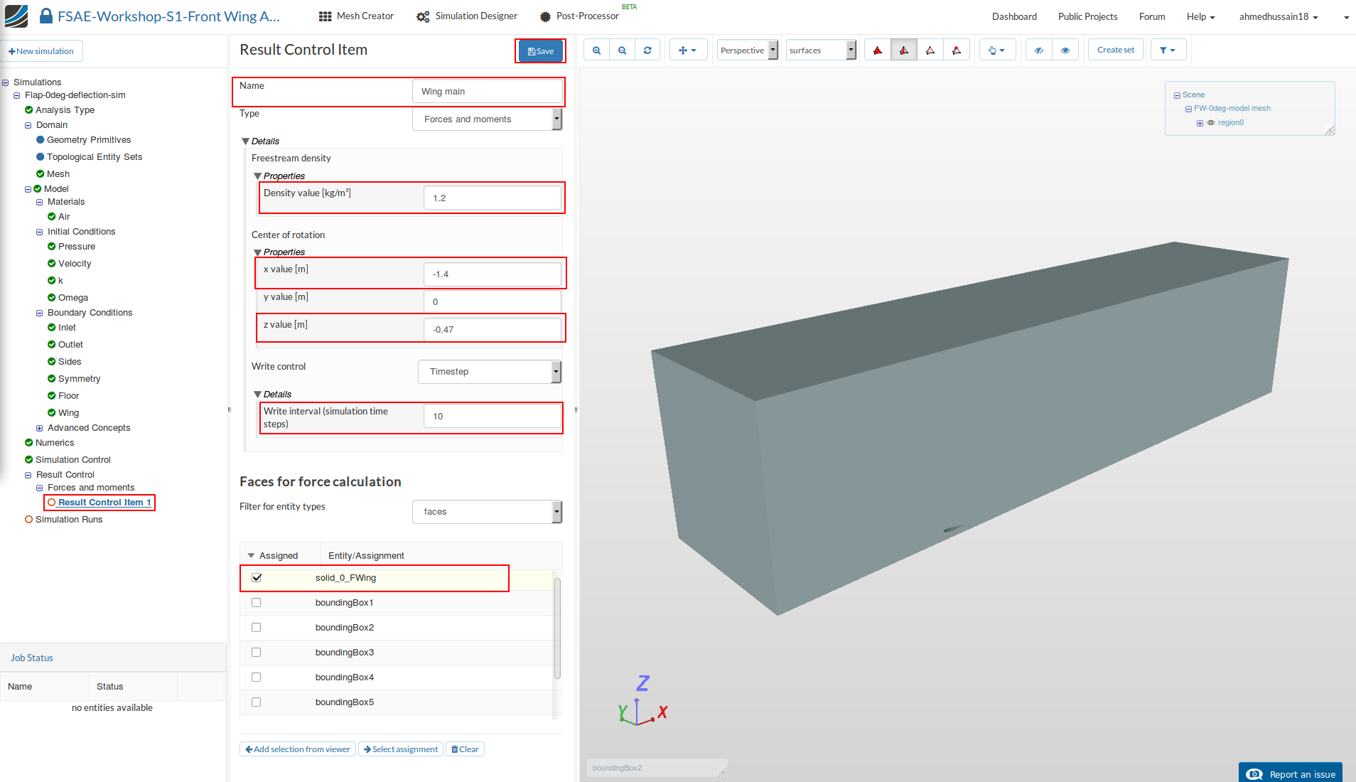
As our last step before running the simulation, we will create result control items in order to get graphical data sets of interest. Firstly, we will create the result control item for the forces and moments.
Go to Result Control and click New next to Forces and Moments.
A new force and moment result control item will be created. Rename it to Wing main (optional).
Then change Density value [kg/m³], x value [m], z value [m] and Write interval (simulation time steps) to 1.2, -1.4, 0.47 and 10 respectively.
Select solid_0_FWing under Faces for force calculation and click Save to register your changes.
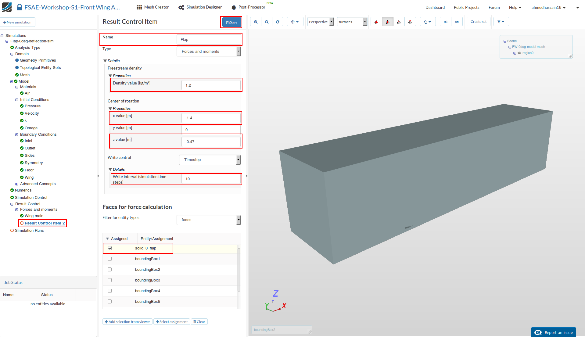
Create another force and moment result control item and rename it to Flap (optional). Change the same values as defined above but this time select solid_0_flap under Faces for force calculation.
Click Save to save your changes.
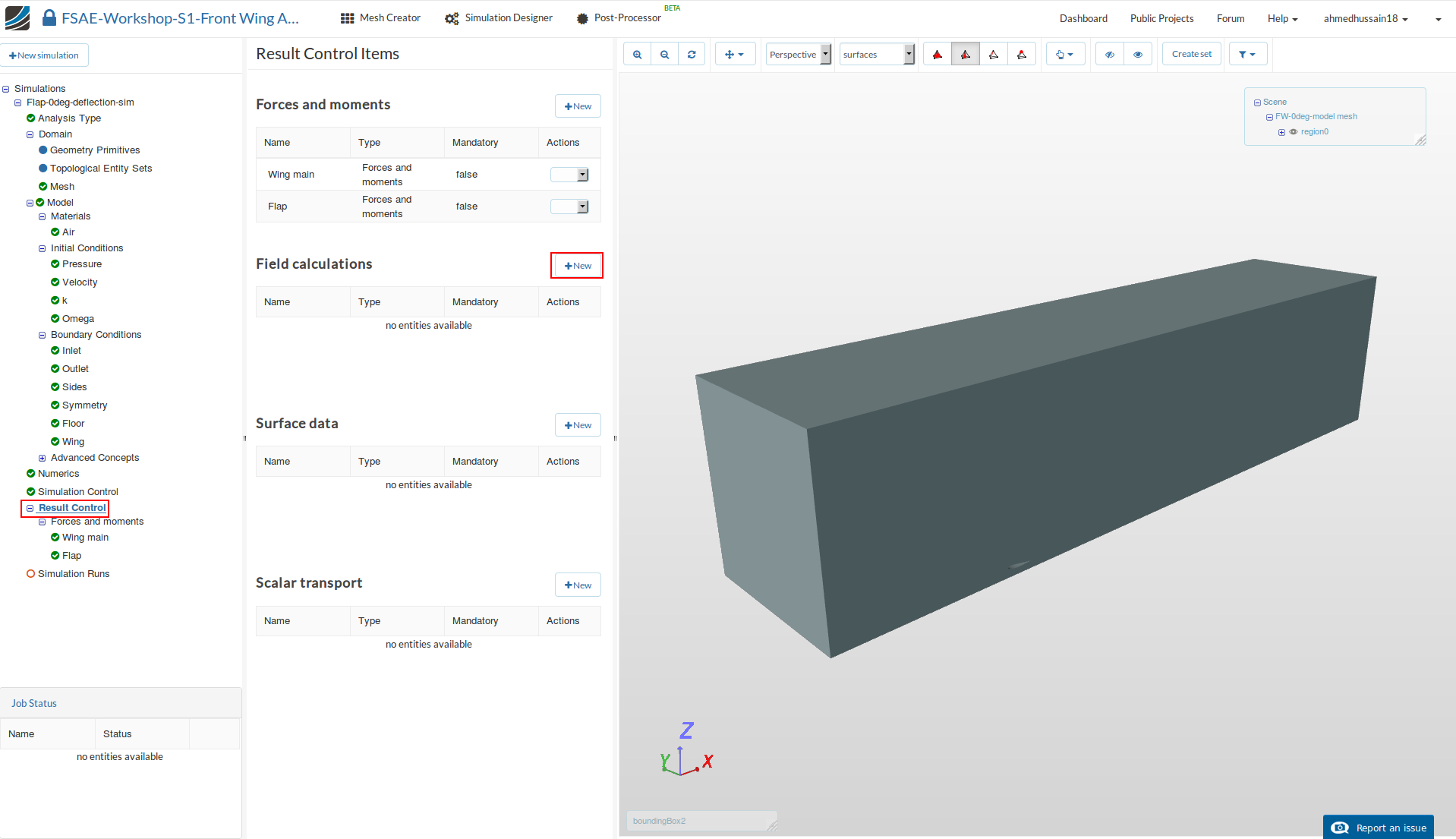
Next, we will create the field calculation items. For this go back to Result Control and click New next to Field calculations.
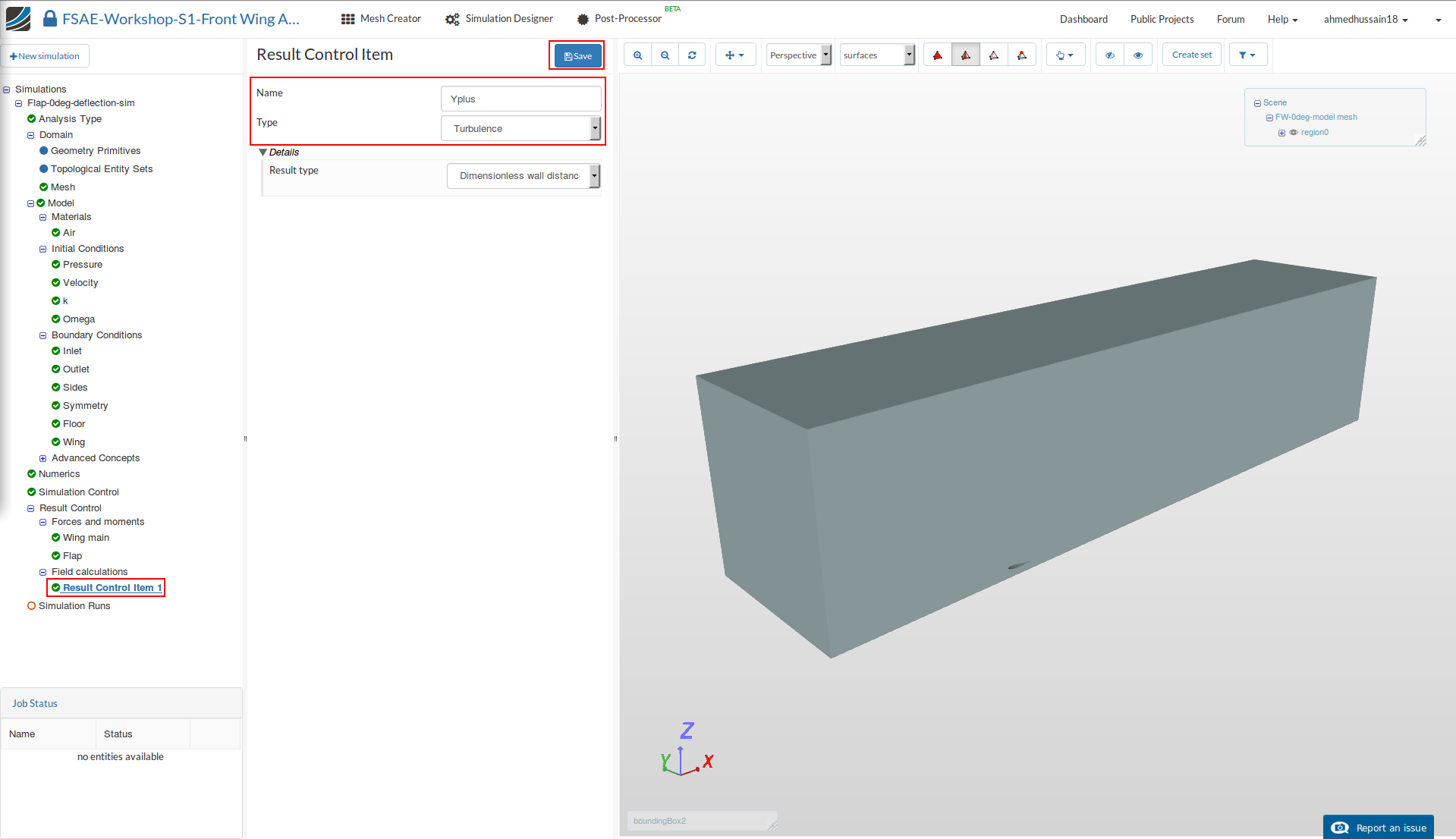
Rename the newly created field calculation item to Yplus (optional).
Change the Type to Turbulence and click Save to register your changes.
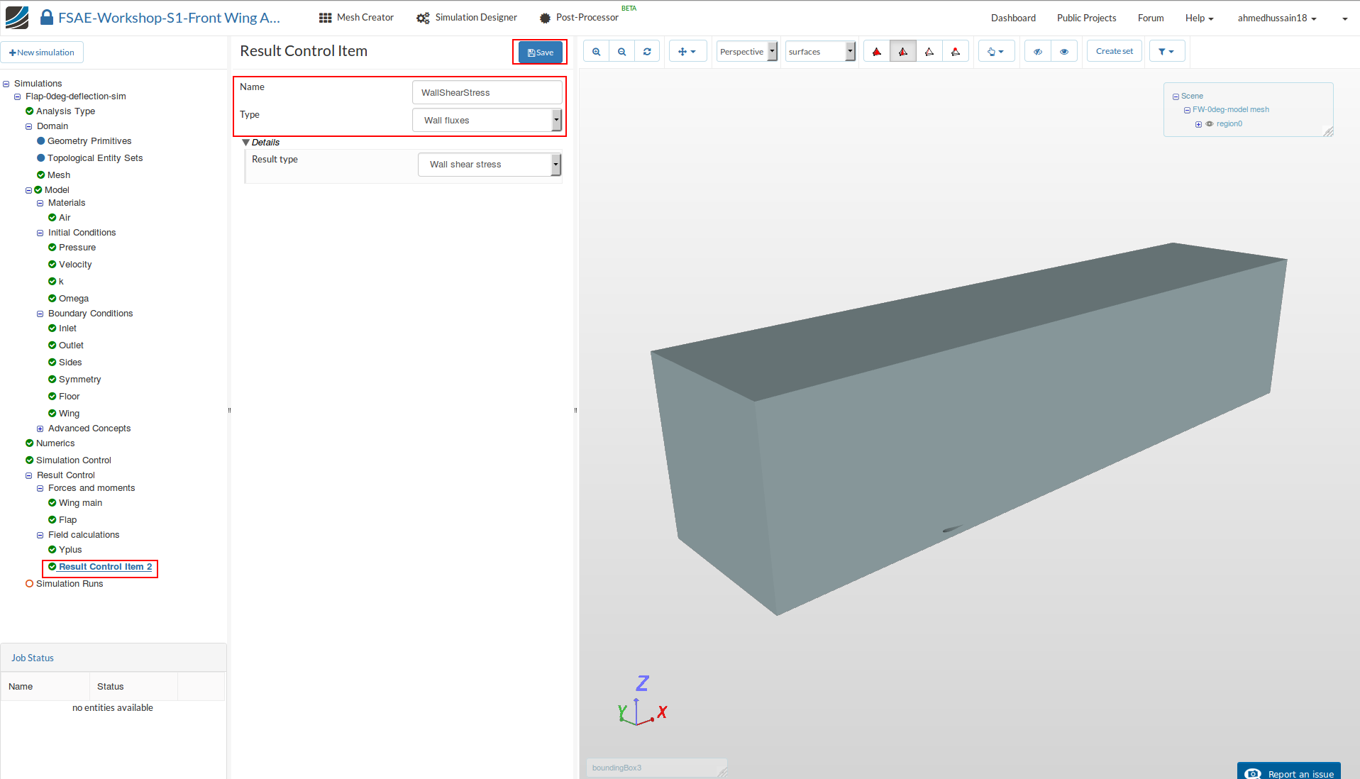
Create another field calculation item and rename it to WallShearStress (optional).
Change the Type to Wall fluxes and click Save to register your changes.
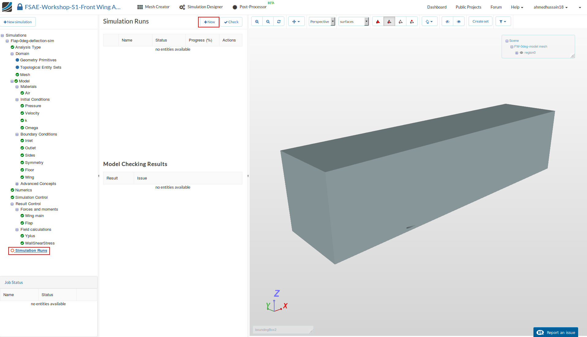
Simulation Run
Once all the above steps are defined, we will proceed to create our first simulation run. Go to Simulation Runs and click on New.
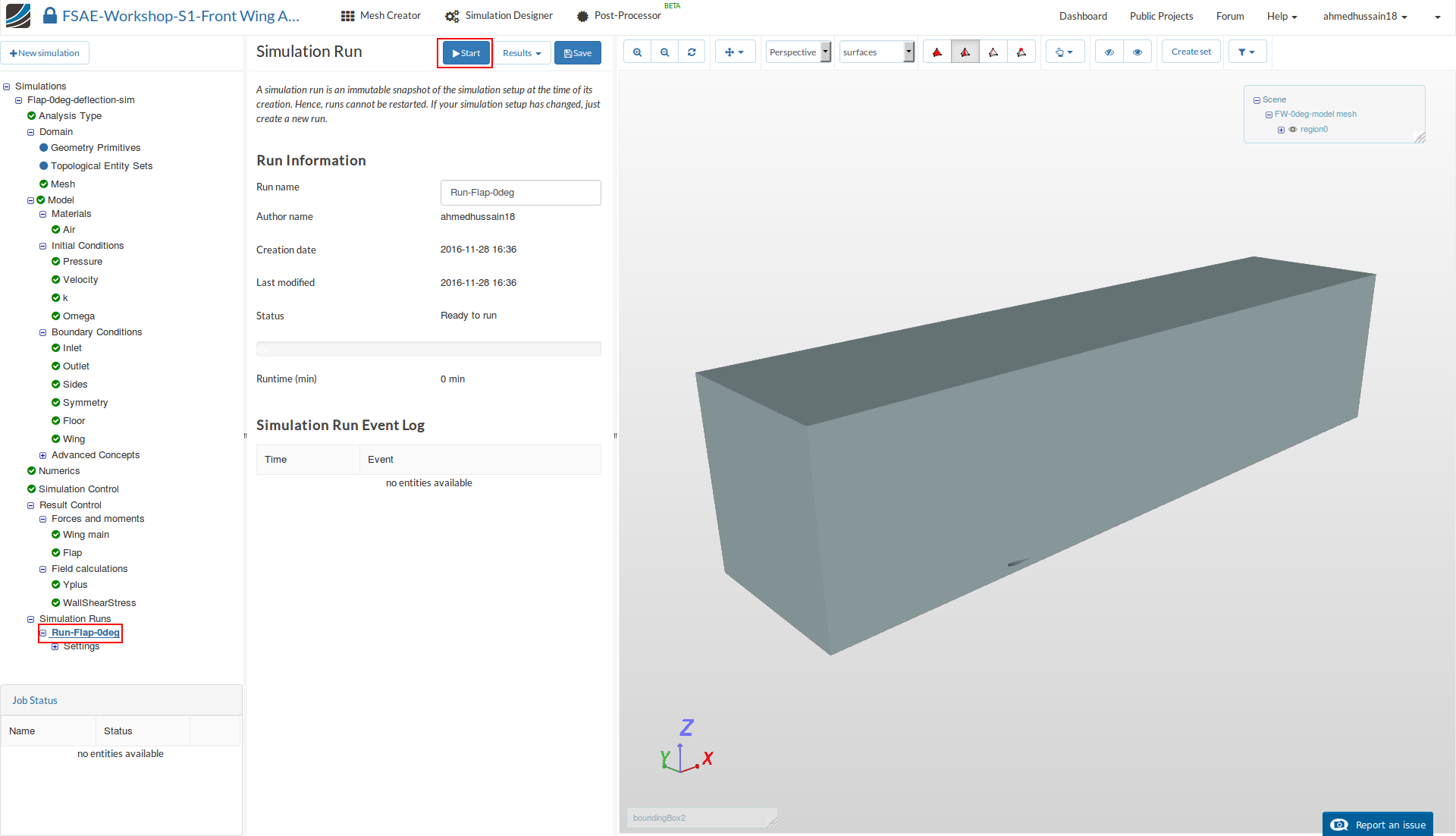
A window will pop up, give a reasonable name to the run e.g. Run-Flap-0deg in this case (optional) and click Create in order to create a new run.
After the run is created, click Start to start the created run. The simulation run can take up to ~120 minutes (~2 hrs.).
Additional Simulation Runs
While the first simulation job is running, take advantage of the parallel computing and proceed to start setting up all the other configurations. You don’t have to perform all the simulation set up operations again from scratch. Just duplicate the already created simulation by right clicking on it and then click Duplicate.
Rename the duplicated simulation to FW-XXdeg-deflection-sim (where XX is the flap degrees) and assign your new domain to the duplicated simulation under Domain.
Then click Save. Now you have to just assign back all the entities to the material, boundary conditions and result control force plot items and then start the simulation job.
When your simulation is completed, proceed to Post-Processor tab in order to post-process your results.
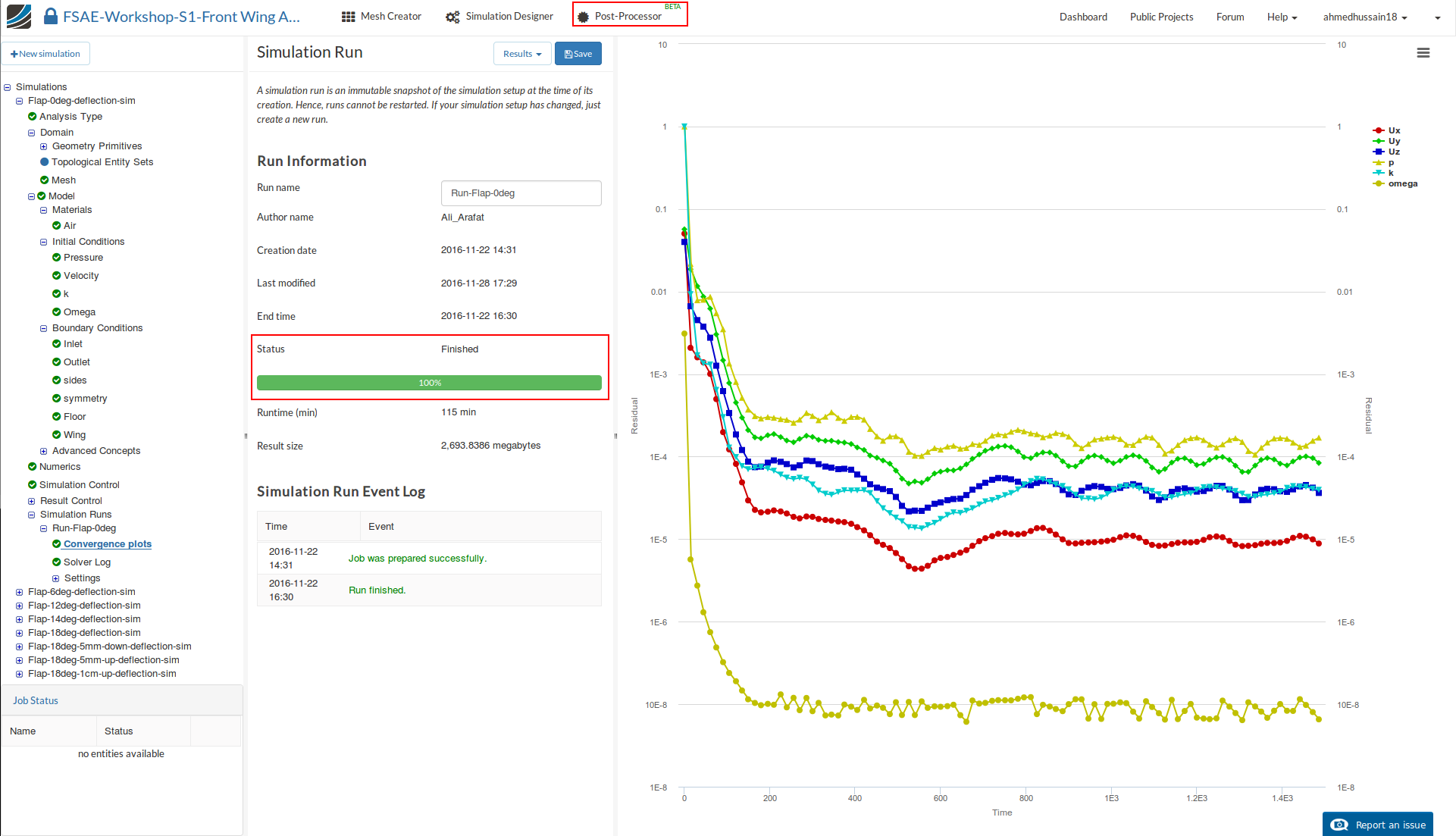
Post-processing
We will show the post-processing only for the first simulation results. You can then follow the same steps in order to post-process other configuration results
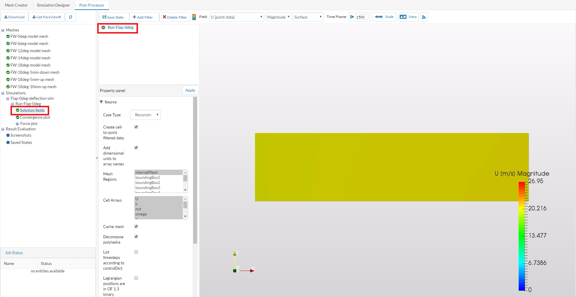
Once in Post-Processor, click on Solution fields under Run-Flap-0deg in order to load the results in viewer. Due to fine mesh it can take up to 5 minutes to load the results in to the viewer.
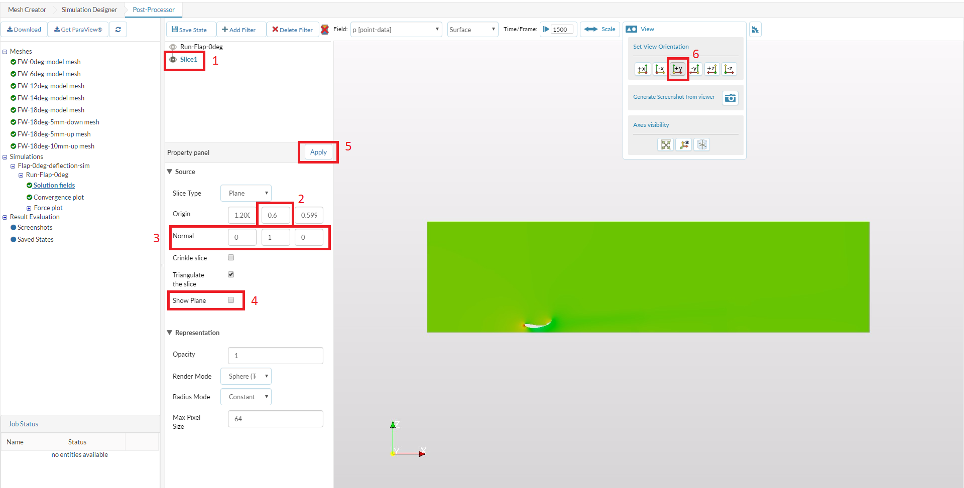
For faster and efficient reviewing of the results, we will use slice filter. In order to add the filter, do the following:
-
Go to Add Filter and select Slice
-
Change Origin middle value i.e. y value to 0.6
-
Change Normal to (0,1,0)
-
Uncheck Show Plane.
-
Click Apply to save the changes.
-
Next set camera orientation to +Y from the View tool over the viewer to get a proper view.
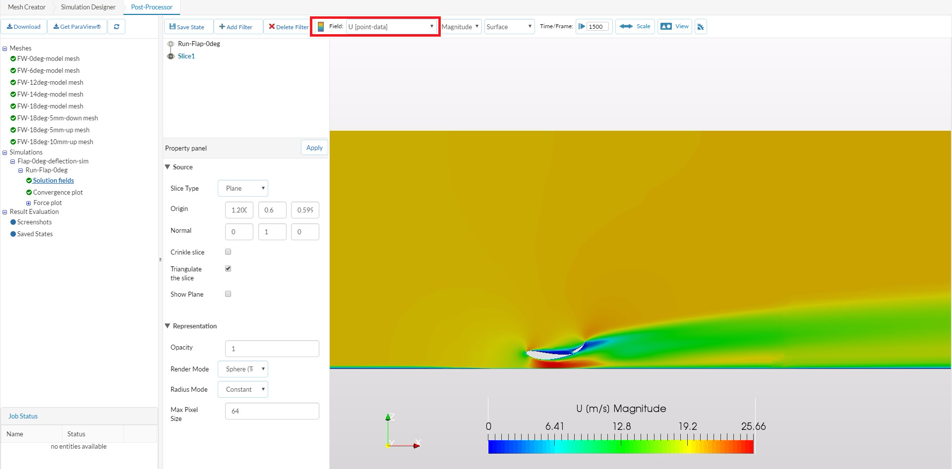
Next change the Field to U [point-data] in order to see the velocity field. Zoom the results with the mouse roller and drag from middle mouse button to get a reasonable view. Turn on the color bar and drag it by holding mouse left button to the bottom.
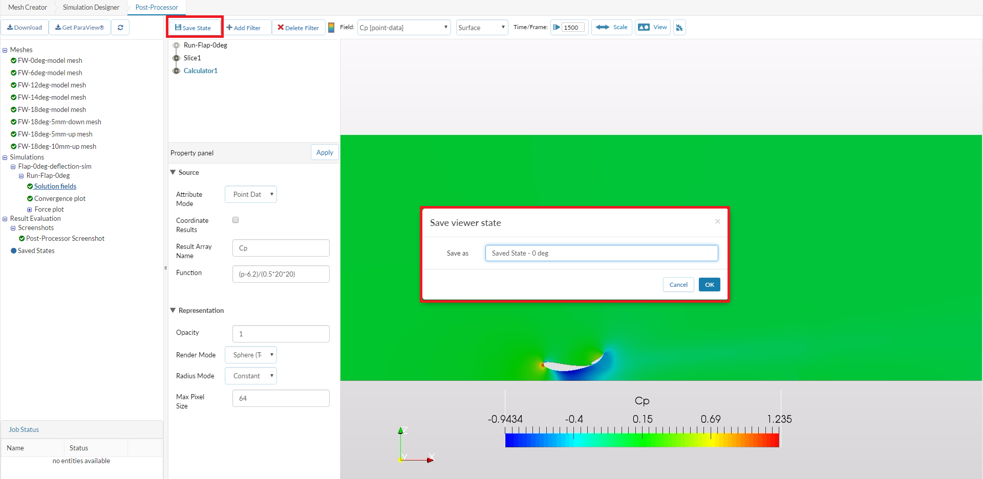
Next we will plot the pressure coefficient. Since this field doesn’t exist therefore we need to create one. First uncheck the colorbar (important; if you don’t do it, you may end up with two different colorbars in the next step) then select Calculator from Add Filter.
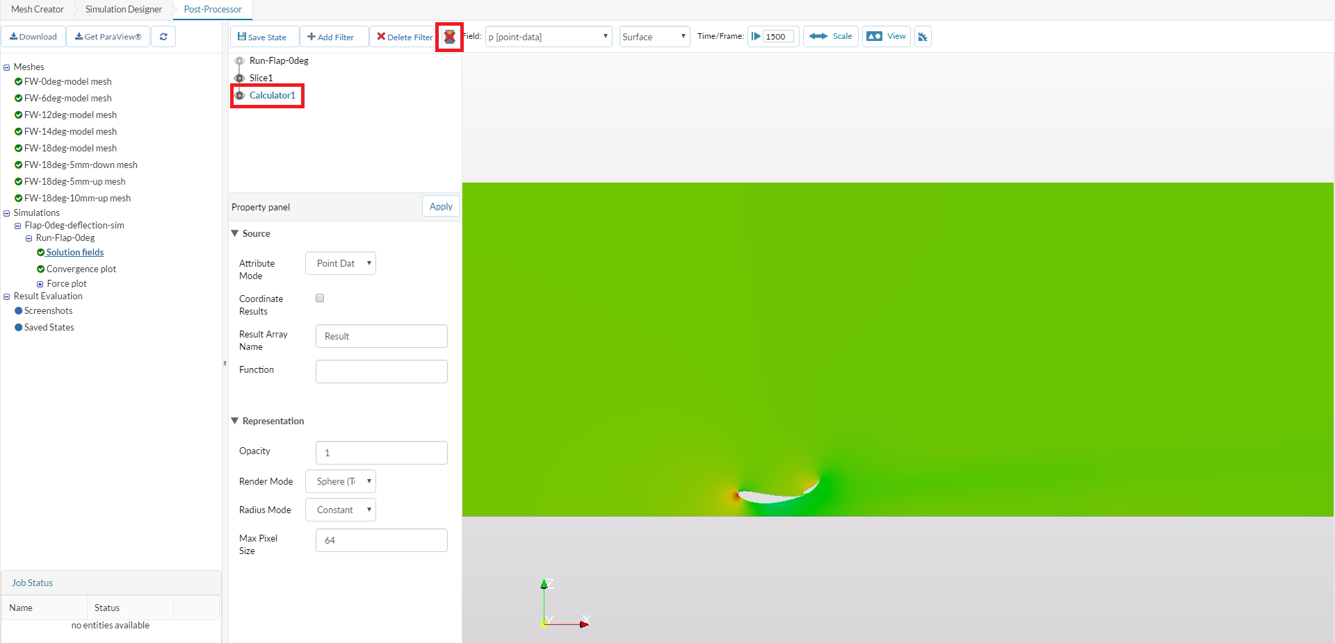
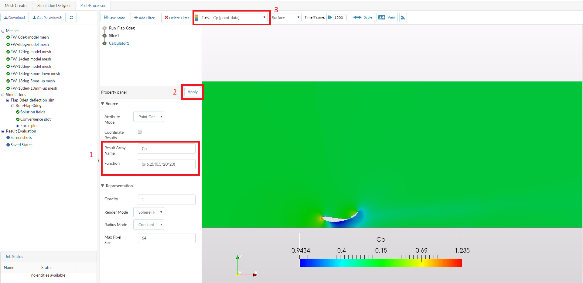
Once the calculator filter is added:
-
Change the Result Array Name and Function to Cp and (p-6.2)/(0.52020) respectively.
-
Click Apply to create a pressure coefficient field.
-
Change Field to Cp[point-data] to see the results.
If you want to take a screenshot of your results, click on the camera icon under View tools. Your screenshot will appear under Result Evaluation section.
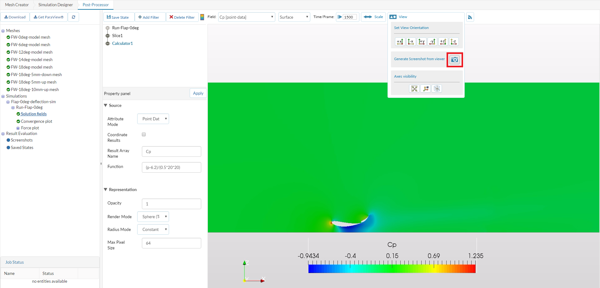
Furthermore, in order to save the state for later use, click on the Save State button. A window will pop up, give a reasonable name e.g. Saved state - 0deg (optional) in this case. Your saved state will also appear under Result Evaluation section.
Lastly to see the plotted data requested beforehand during the simulation setup, switch over to WingMain under the Force plot.
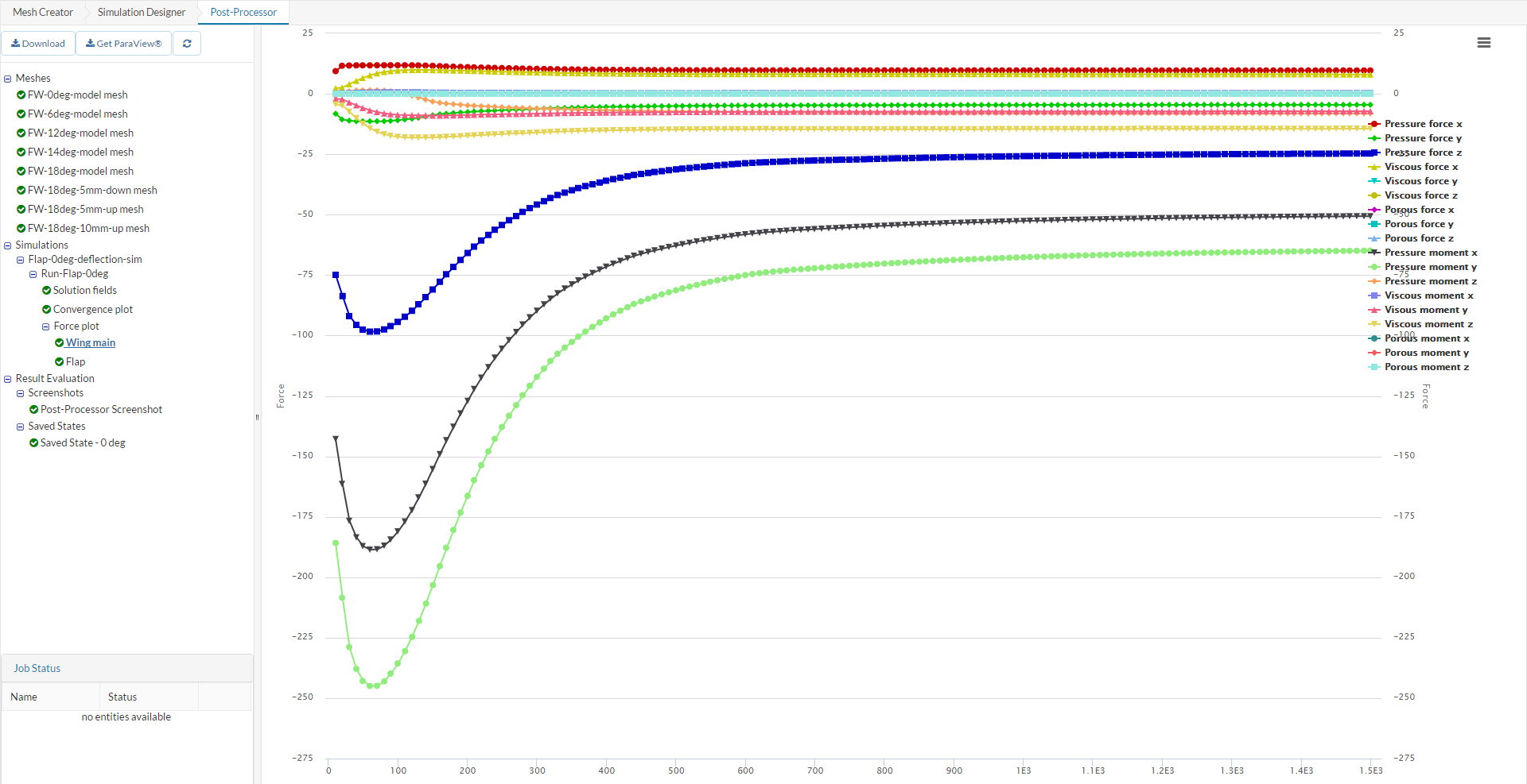

 Unfortunately for now its not possible. Each plotting feature of Paraview need some more improvements and modifications in online version. Therefore, needs sometime but we are looking forward to it.