Recording

Exercise
Choosing the right numerical settings can help to greatly decrease the computational effort required to run a simulation. However, there are a trade-offs between stability and speed of the numerical calculation.
The aim of this exercise is to investigate the impact of different numerical settings on the overall simulation time.
Step-by-Step Instructions
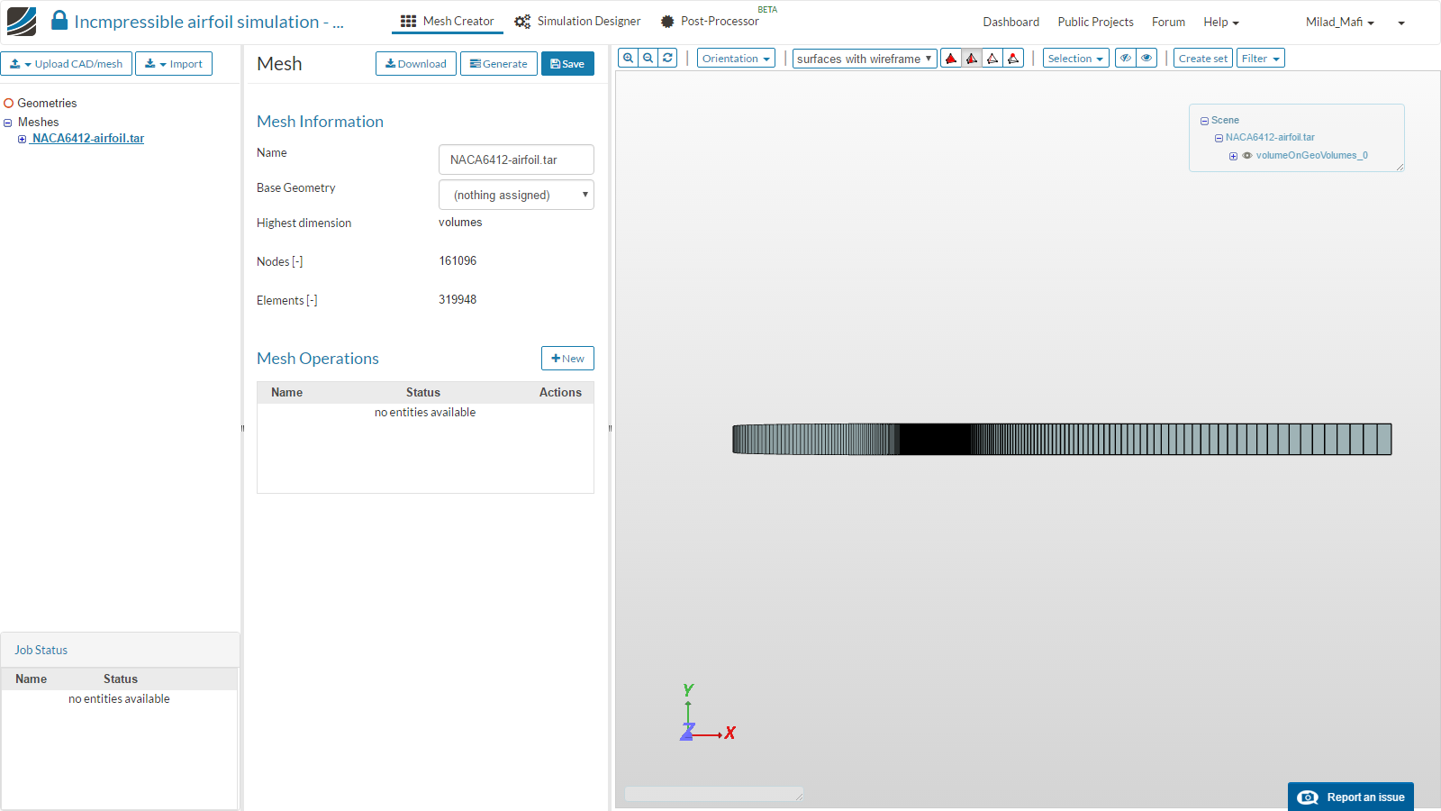
- For this project we will use an imported mesh for our simulation. Click here to import the project. The project contains one mesh which will be used for this session.
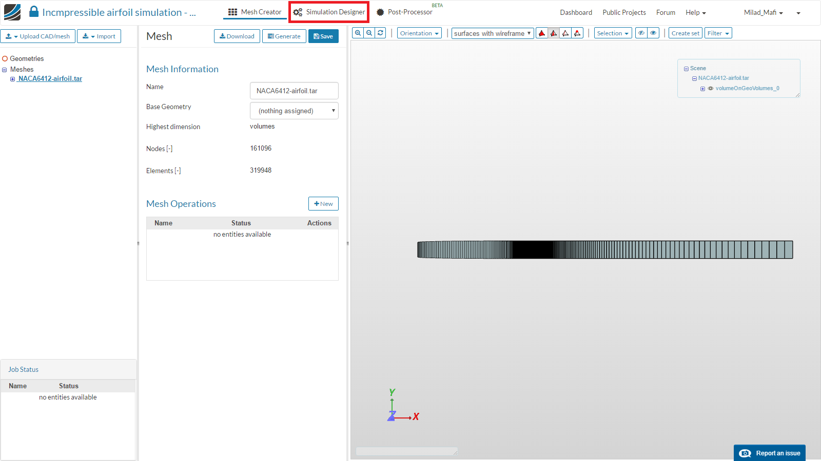
- For settings up the simulation switch to the Simulation Designer tab.
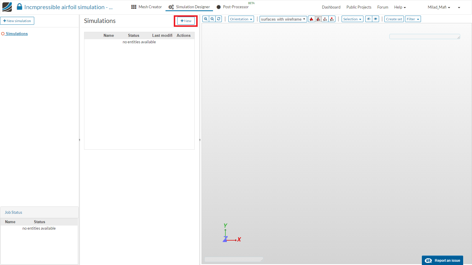
- Next, click New simulation to create a new simulation item in the Project Tree.

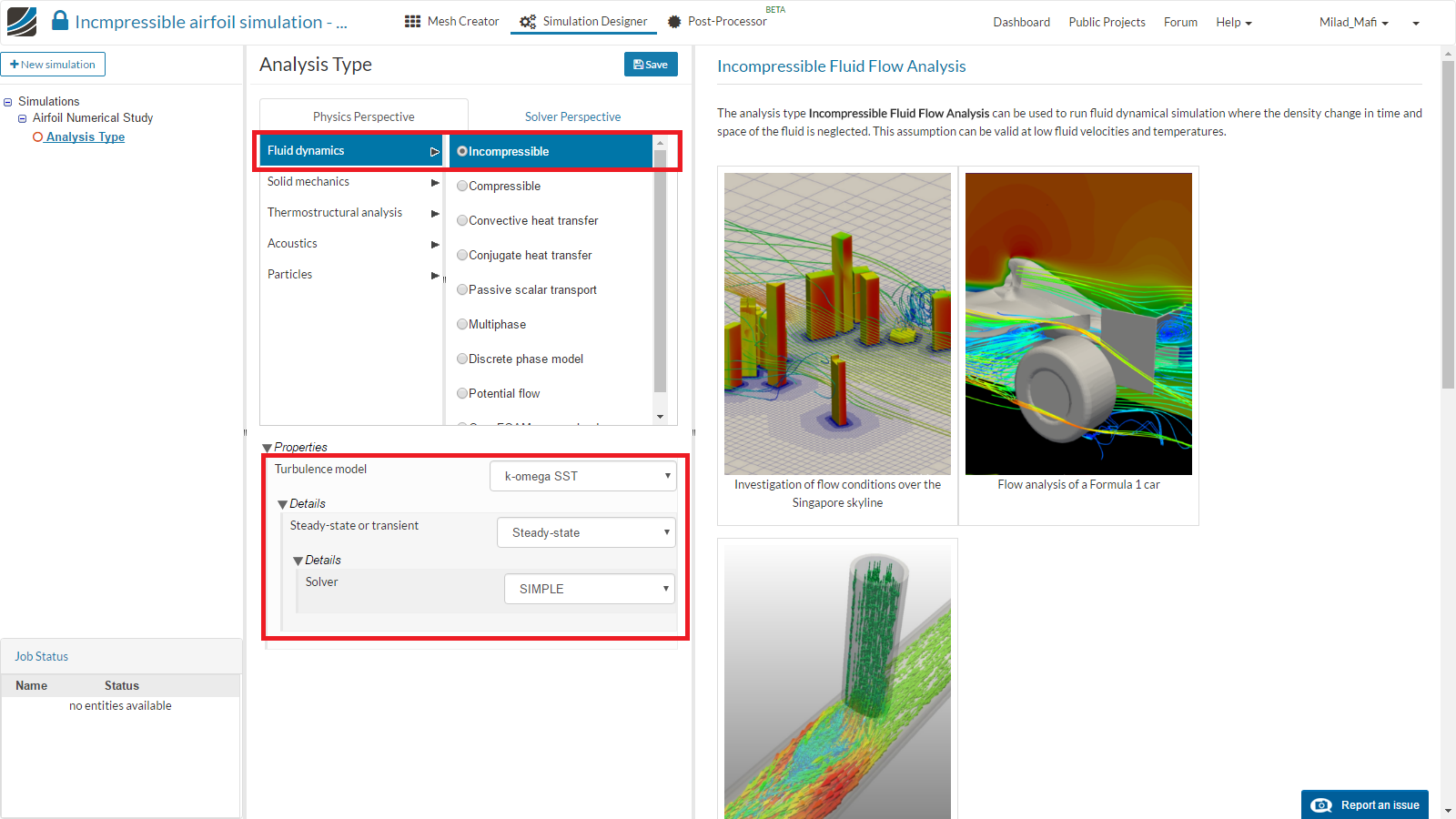
- From the middle column set the Analysis Type to Fluid dynamics and Incompressible. For this analysis we will select K-omega SST for our turbulence model with Steady-state behavior and the SIMPLE solver. Click Save to preserve this selection. You will then see the Project Tree expand with the full setting in the left column.
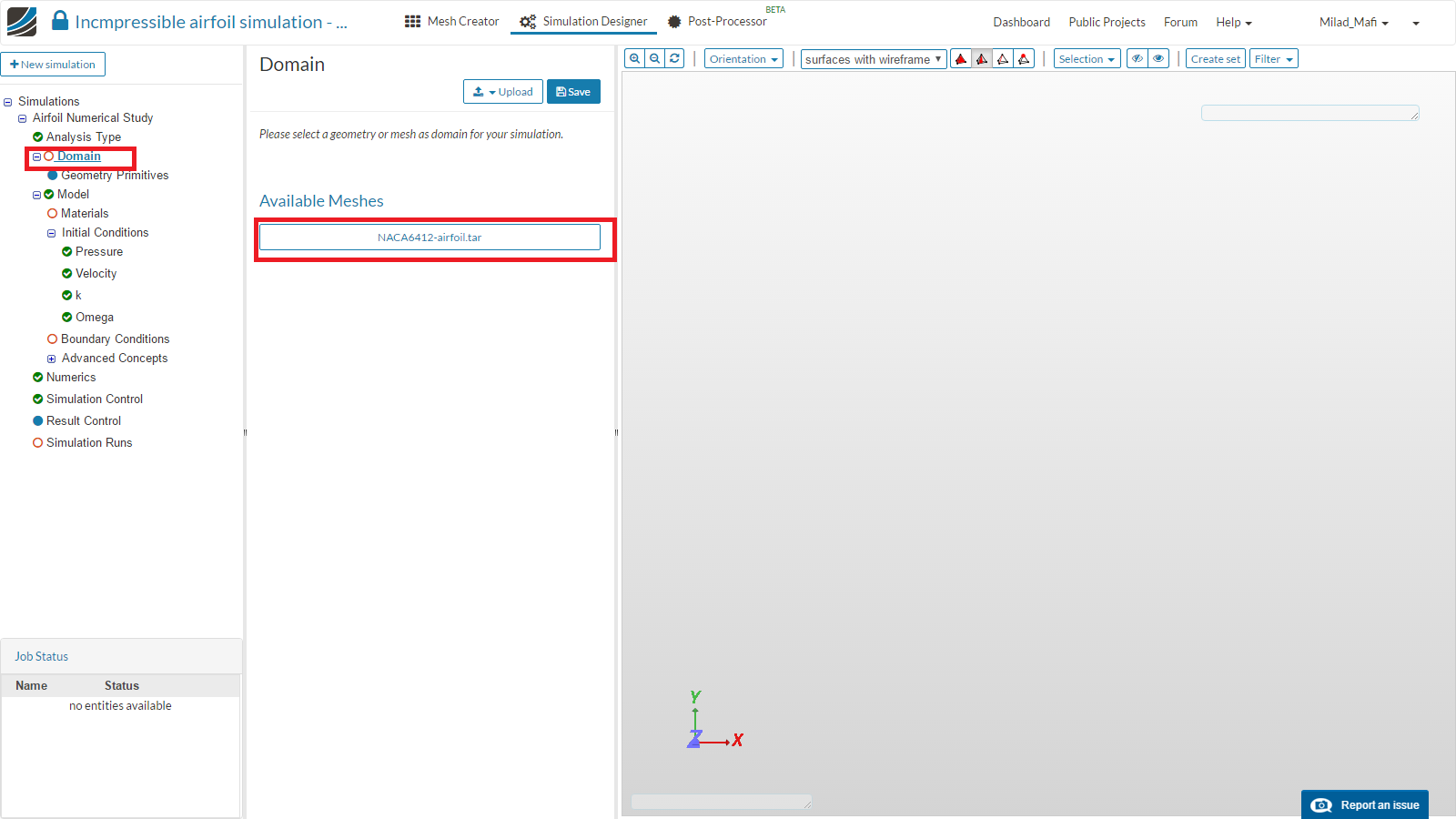
- In the Project Tree move to the domain and assign the respective mesh to the simulation and press Save.
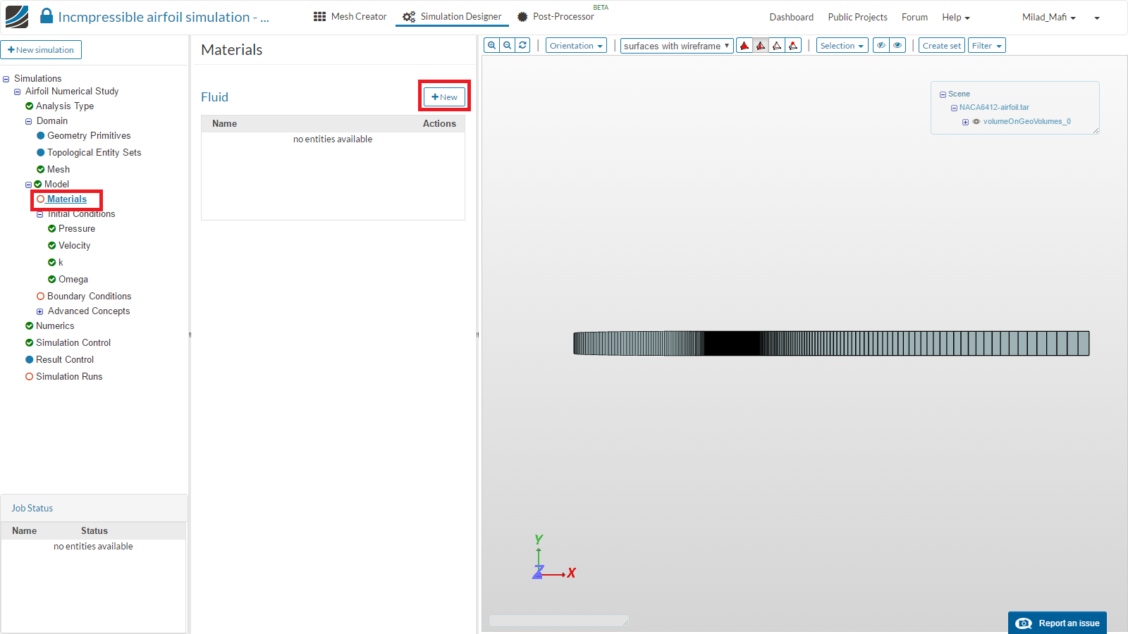
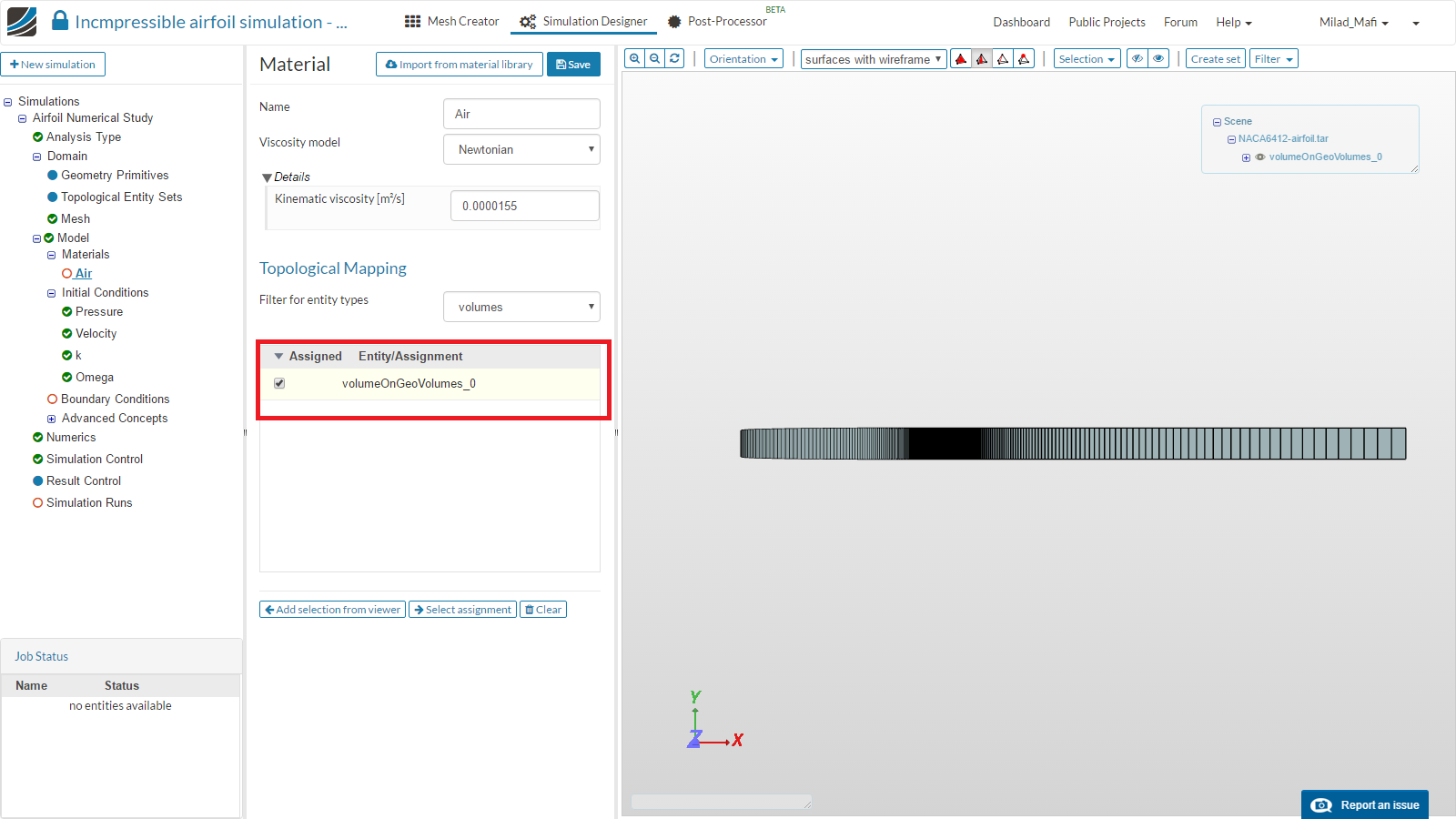
- Move to the Materials item in the Project Tree and click New.
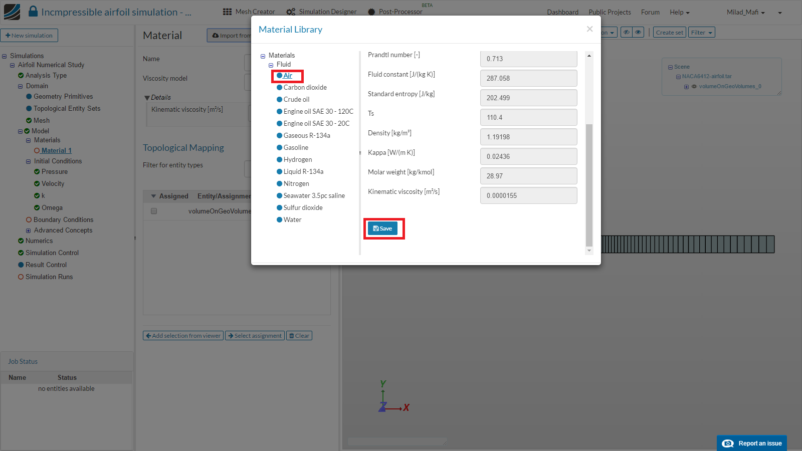
- Import the Air from the material library and assign it to the entire volume.
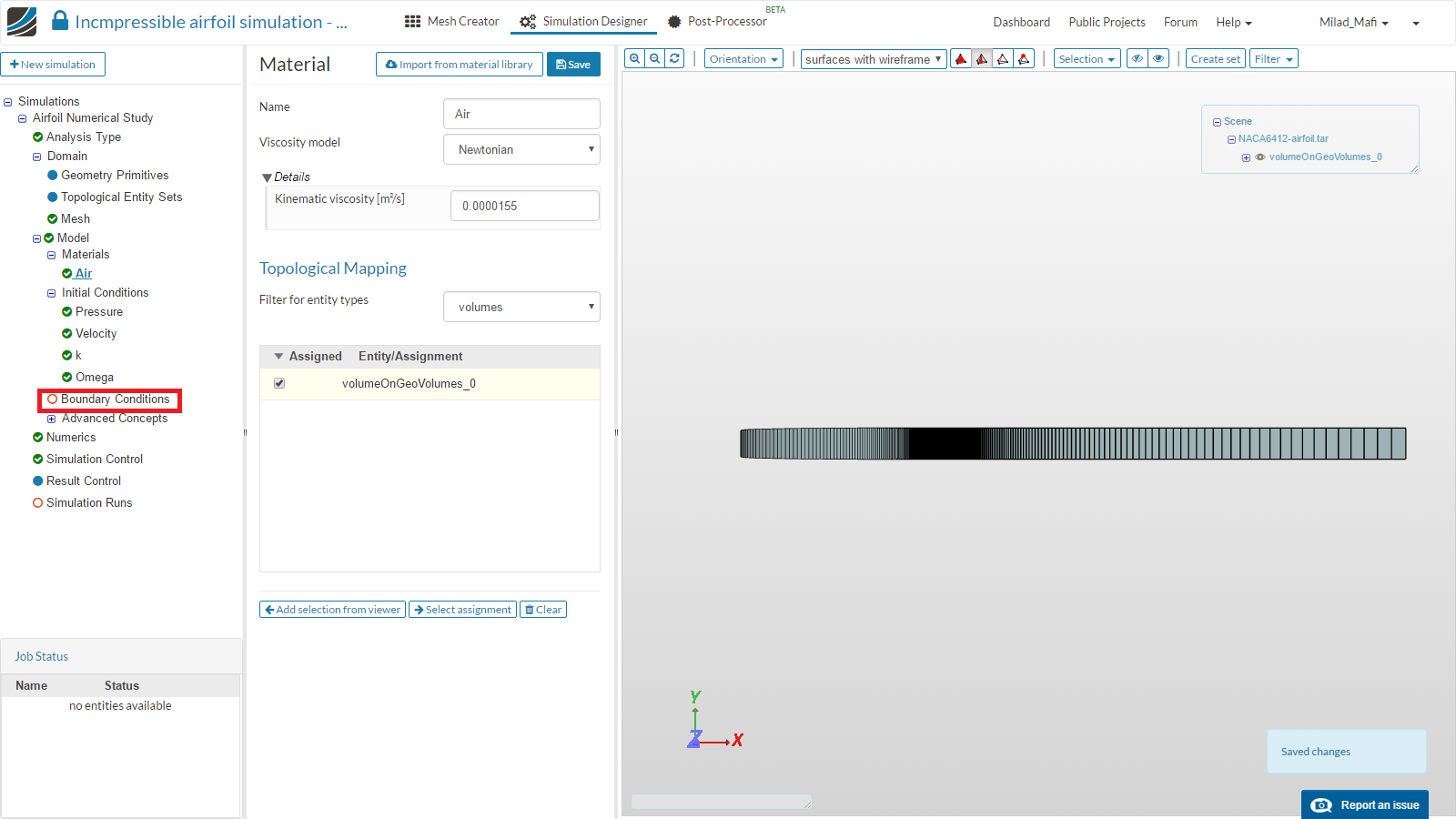
- Move to the Boundary Conditions item in the Project Tree to set the boundary conditions.
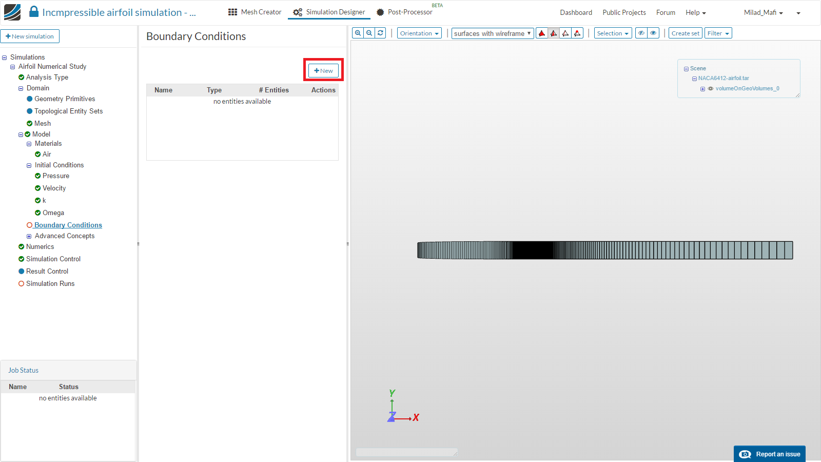
- Click New to add a new boundary condition.
- First add a boundary condition by the name “Inlet”. Set the Type to Velocity Inlet/Fixed Value with an x value of 25m/s and assign it to the face inlet.

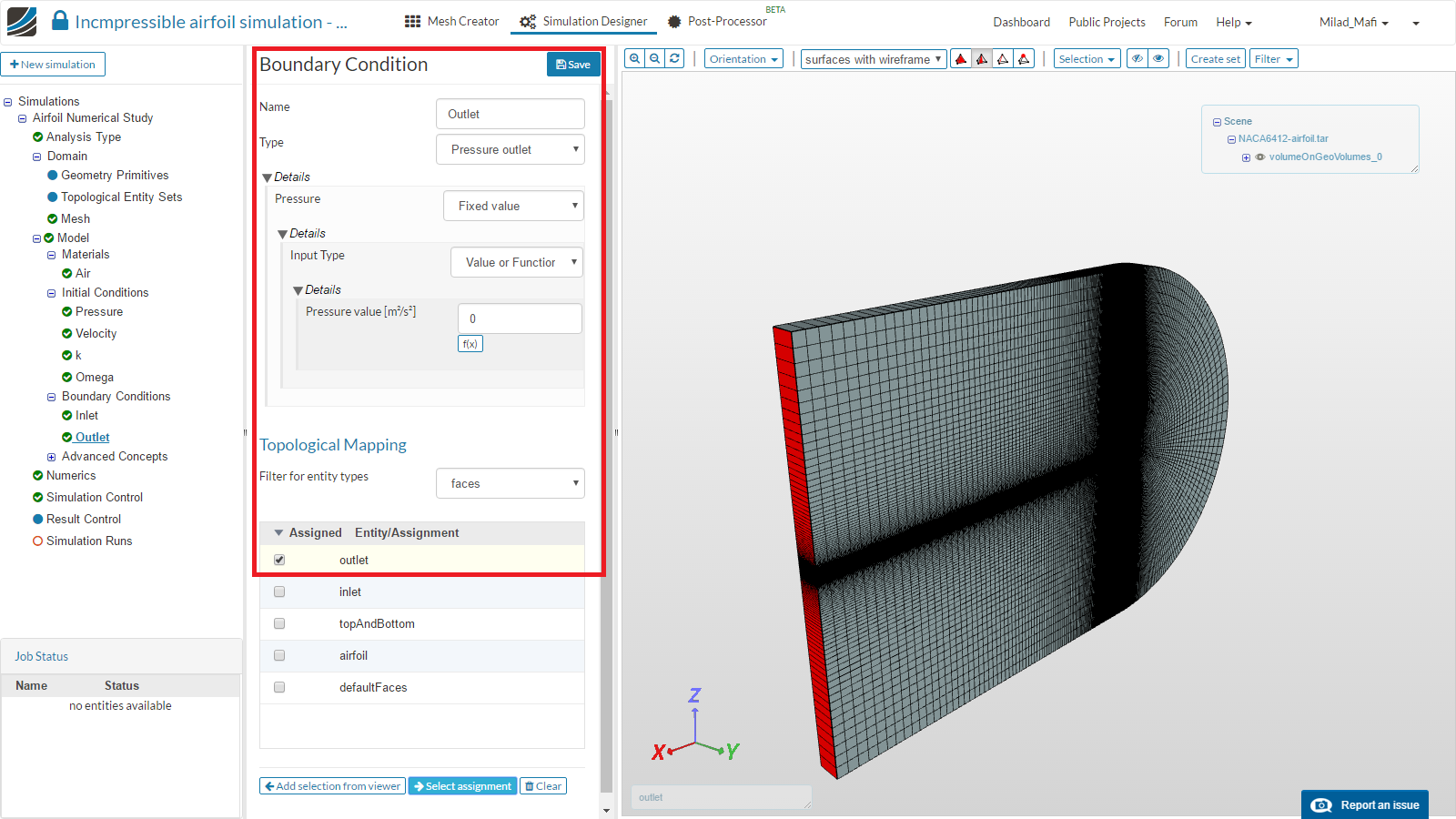
- Add another boundary condition and rename it to “Outlet”. Set the type to Pressure Outlet with a value of 0 and assign it to the face outlet.
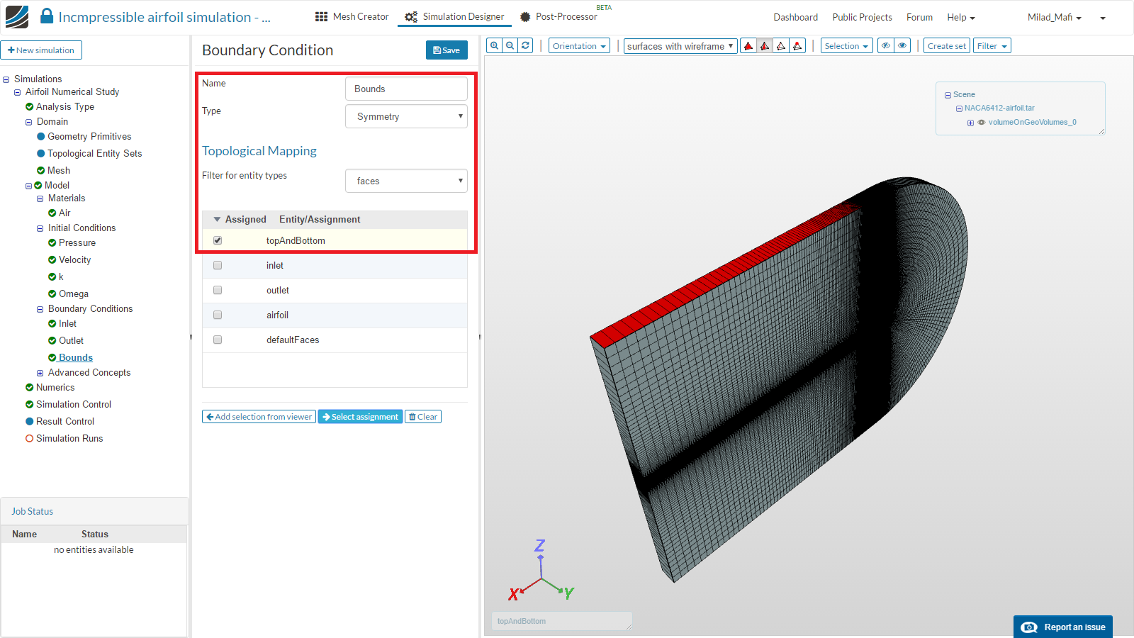
- Next, add another boundary condition and rename it to “Bounds”. Set the type to Symmetry and assign it to the face topAndBottom.
- Since we want to investigate numerical settings, we will run a 2D simulation. For a 2d case, it is necessary to add a specific boundary condition to the surrounding walls. Add another boundary condition and rename it to 2D Dummy. Set the type to Custom and assign it to the face defaultFaces.

- Finally, add the last boundary condition and rename it to “Airfoil”. Set the type to Wall (no slip / wall function) and assign it to the face airfoil.

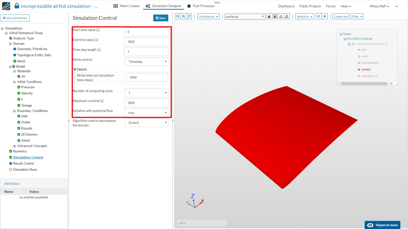
- Now move to the Simulation Control and set the parameters accordingly and then Save
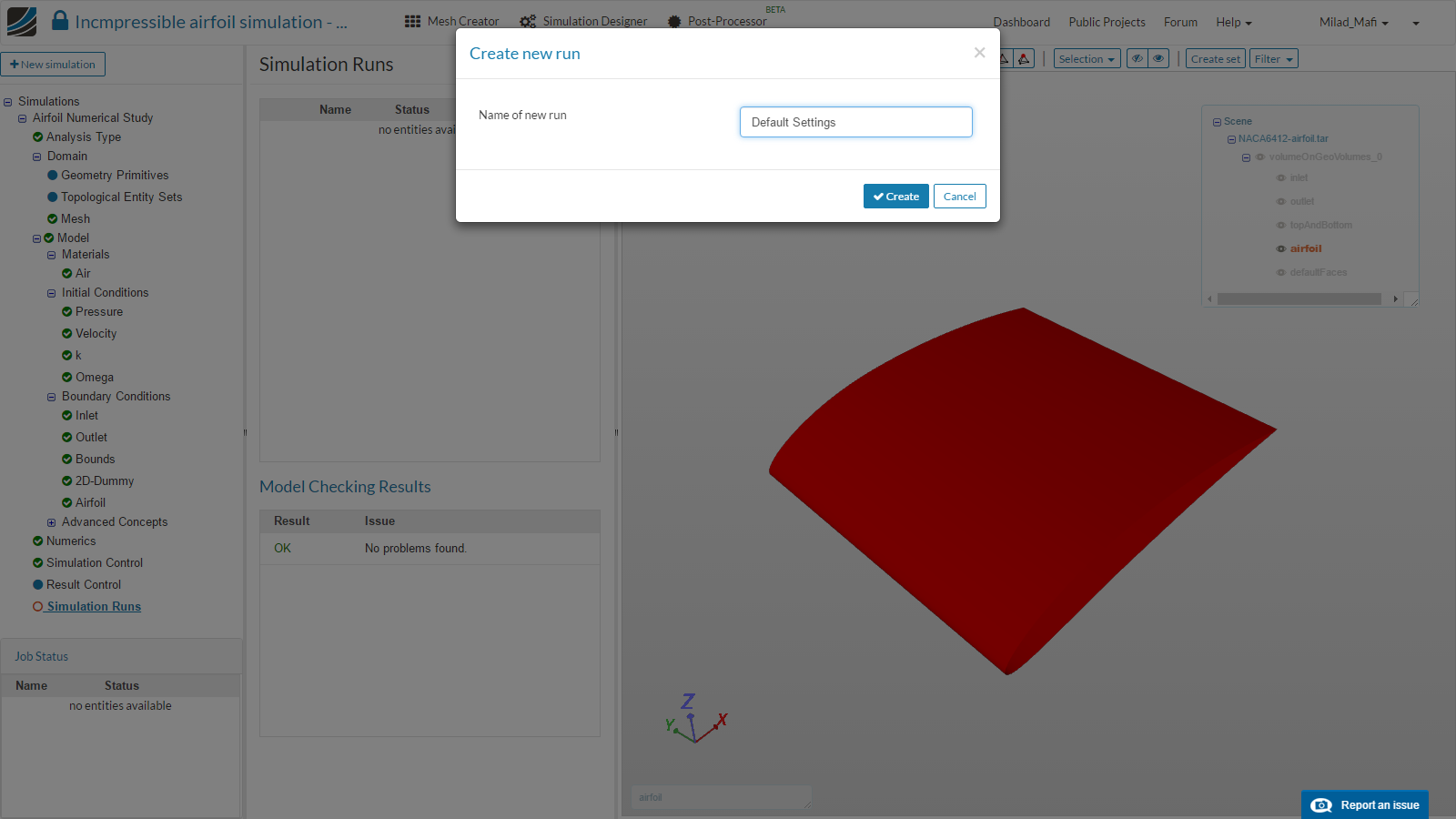
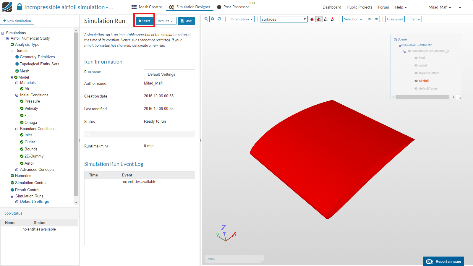
- Click on the Simulation Runs item. Create a new run and name it. Finally click Start to run the simulation.

-
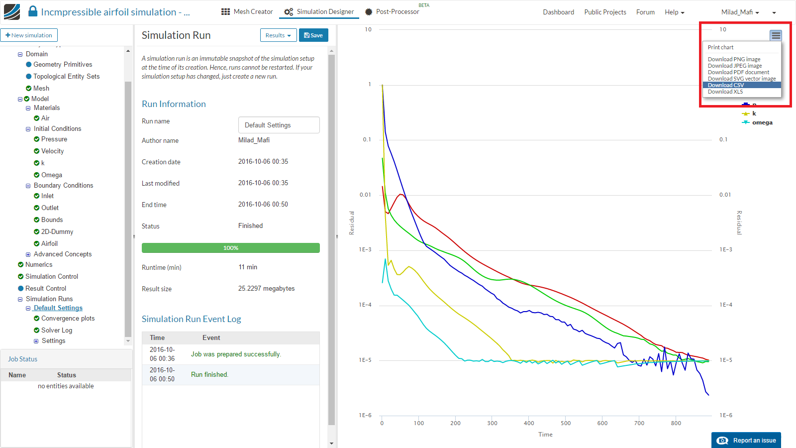
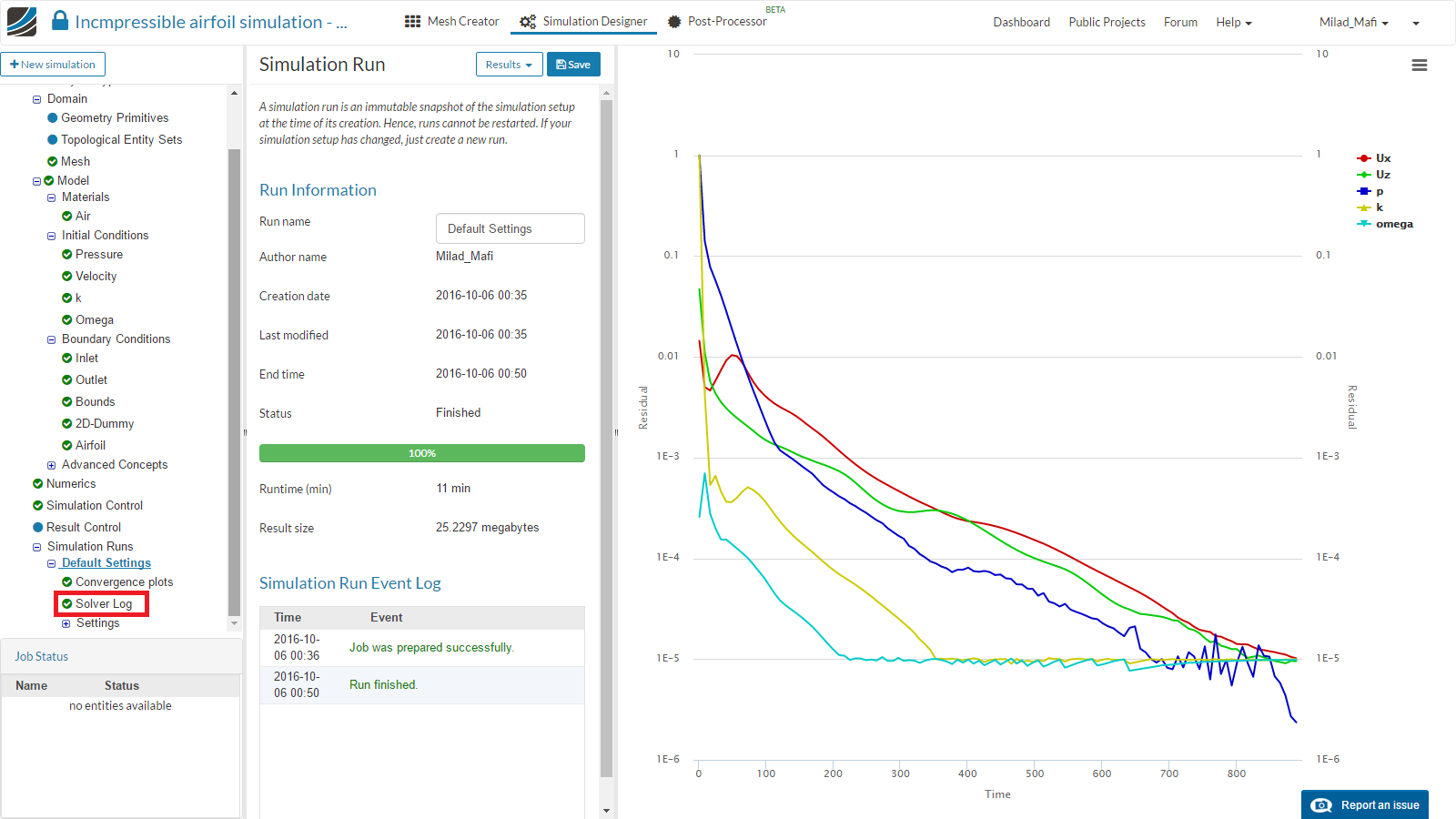
Once the simulation is finished, you can check the run time and number of iterations which were needed for the convergence criteria to be reached.
-
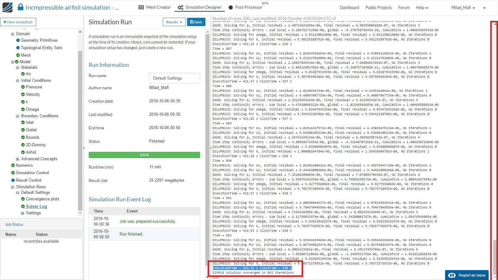
To see this information, click on the’Solver Log item in the project tree. This will open the log file of the solver.
- We will now change numerical settings and examine the effect on the calculation time and number of iterations till convergence.
Relaxation
Relaxation and Convergence Criteria
Numerical methods used to solve the equations for fluid flow and heat transfer most often employ one or more iteration procedures. By their nature, iterative solution methods require a convergence criteria that is used to decide when the iterations can be terminated.
In many cases, iteration methods are supplemented with relaxation techniques. For example, over-relaxation is often used to accelerate the convergence of pressure-velocity iteration methods, which are needed to satisfy an incompressible flow condition. Under-relaxation is sometimes used to achieve numerically stable results when all the flow equations are implicitly coupled together.
Choosing Relaxation Criteria
The amount of over or under-relaxation used can be critical. Too much leads to numerical instabilities, while too little slows down convergence. Similarly, a poorly chosen convergence criteria can lead to either poor results (when too loose) or excessive computational times (when too tight).
Selecting proper relaxation and convergence criteria can be a difficult and frustrating experience for users of computational fluid dynamics software. The criteria depend on the specifics of the problem being solved, which may change during the evolution of a problem. Unfortunately, there are no universal guidelines for selecting criteria because they depend not only on the physical processes being approximated, but also on the details of the numerical formulation. Many CFD programs have a standard set of recommended criteria, but users must often resort to trial-and-error adjustments to get good results.
source: Flow3D
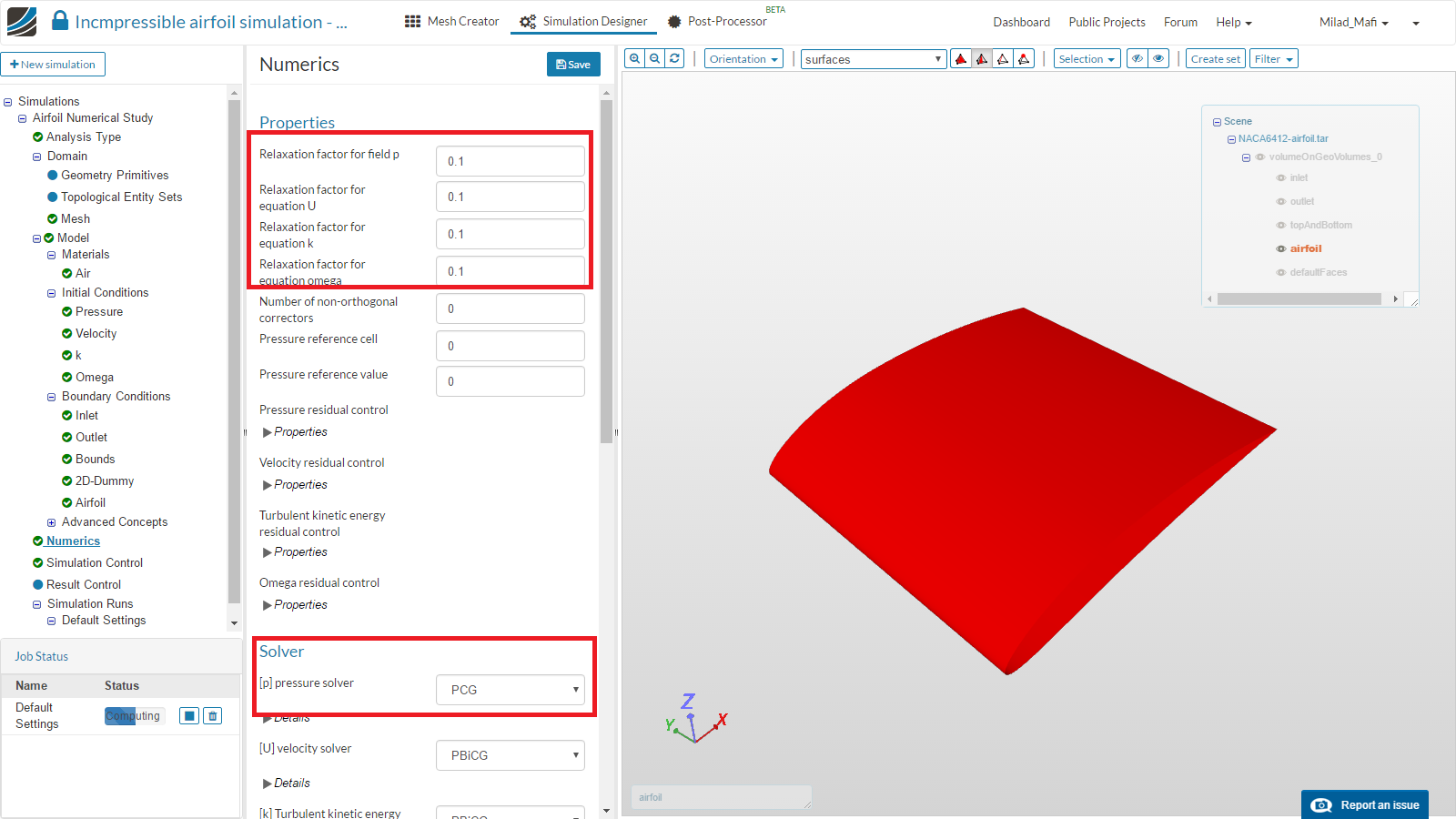
-
We will now change all relaxation factors for p, U, k and omega to a uniform value. In addition, we will change the solver for pressure from GAMG to PCG. Then create a new simulation run and start it.
-
Please create a simulation run for following relaxation values:
0.1, 0.2, 0.3, 0.4, 0.5, 0.6, 0.,7
Solver Tolerances
Just like the simulation result, the single steps the simulation are calculated with iterative methods. So called ‘linear solvers’ are used to calculate the solution of linear equation system. You can find some information about that in the recording of the session. A good example for such a linear solver which is also used on the SimScale platform can be found here:
https://www.youtube.com/watch?v=EoCgoi9Cro0
-
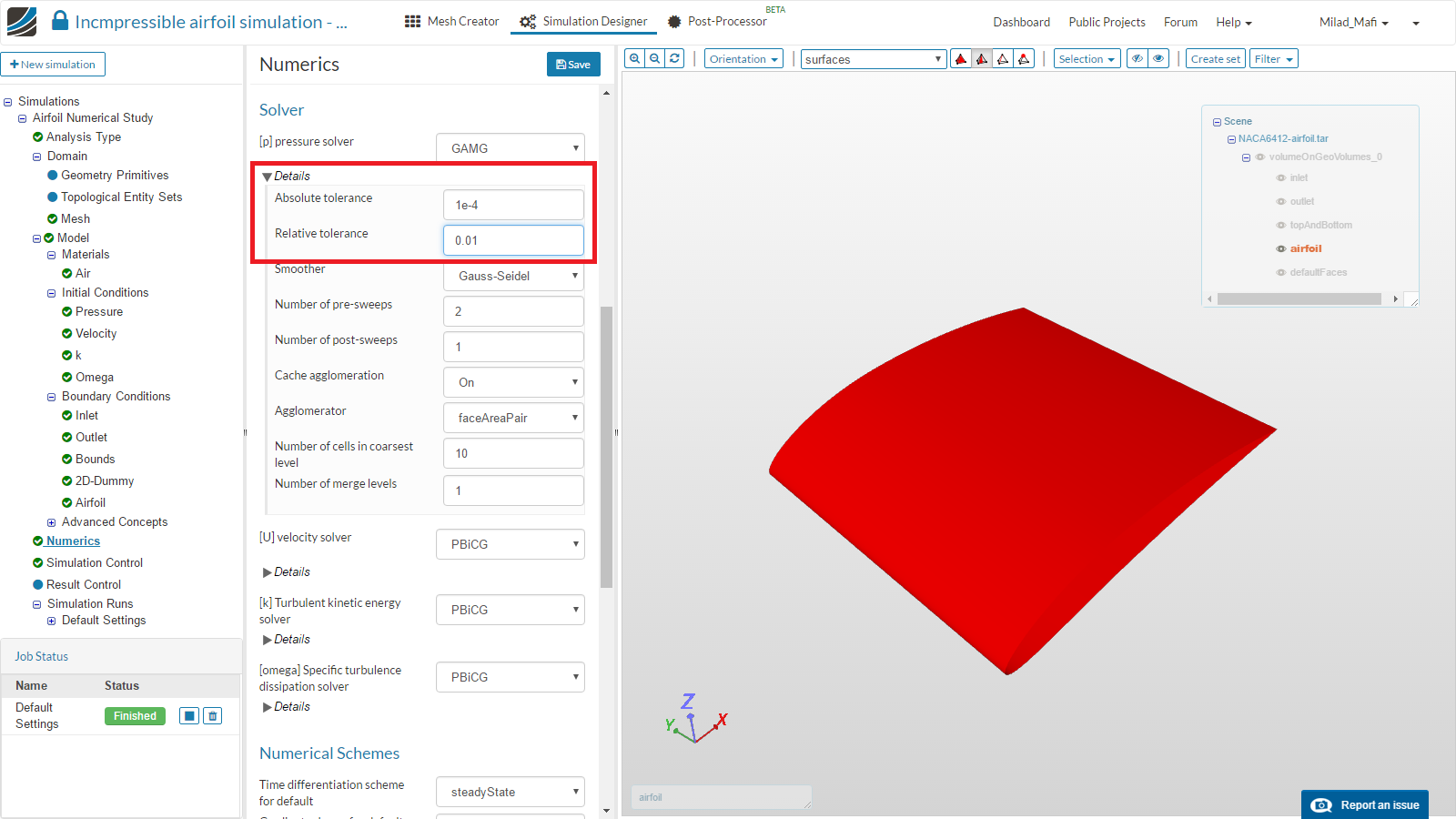
We will now change the tolerance settings of the linear solver for pressure according following values and create a new simulation run.
-
Create a simulation run for following settings (Absolute Tolerance/Relative Tolerance)
(1e-5/0.01), (1e-6/0.01), (1e-7/0.01) -
Note: You need to change back the other values to the initial state manually!
Schemes
Numerical schemes are used to calculate derivatives etc. This topic was also covered during the webinar session. You can find additional information here:
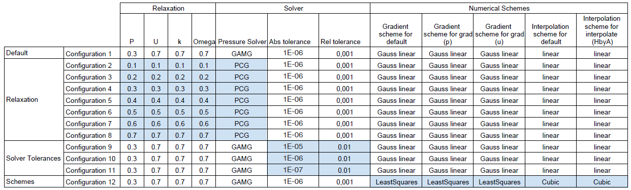
- We will now change all schemes to high order schemes according to the image below. Please create a simulation run for these specific settings.

It total you should have created 1 simulation with 12 different simulation runs as shown in the table below. After the runs are finished you can compare the computation time for different numerical settings.

Table courtesy of: Mario Larreta