Air Conditioning and Ventilation Webinar
Natural convection in a kitchen

Import the project by clicking the link below (Ctrl+click to open in new tab).
Project Link: SimScale Login
Once the project is imported, the workbench is automatically opened. Then follow the steps below for setting up a convective heat transfer simulation.
Step-by-Step
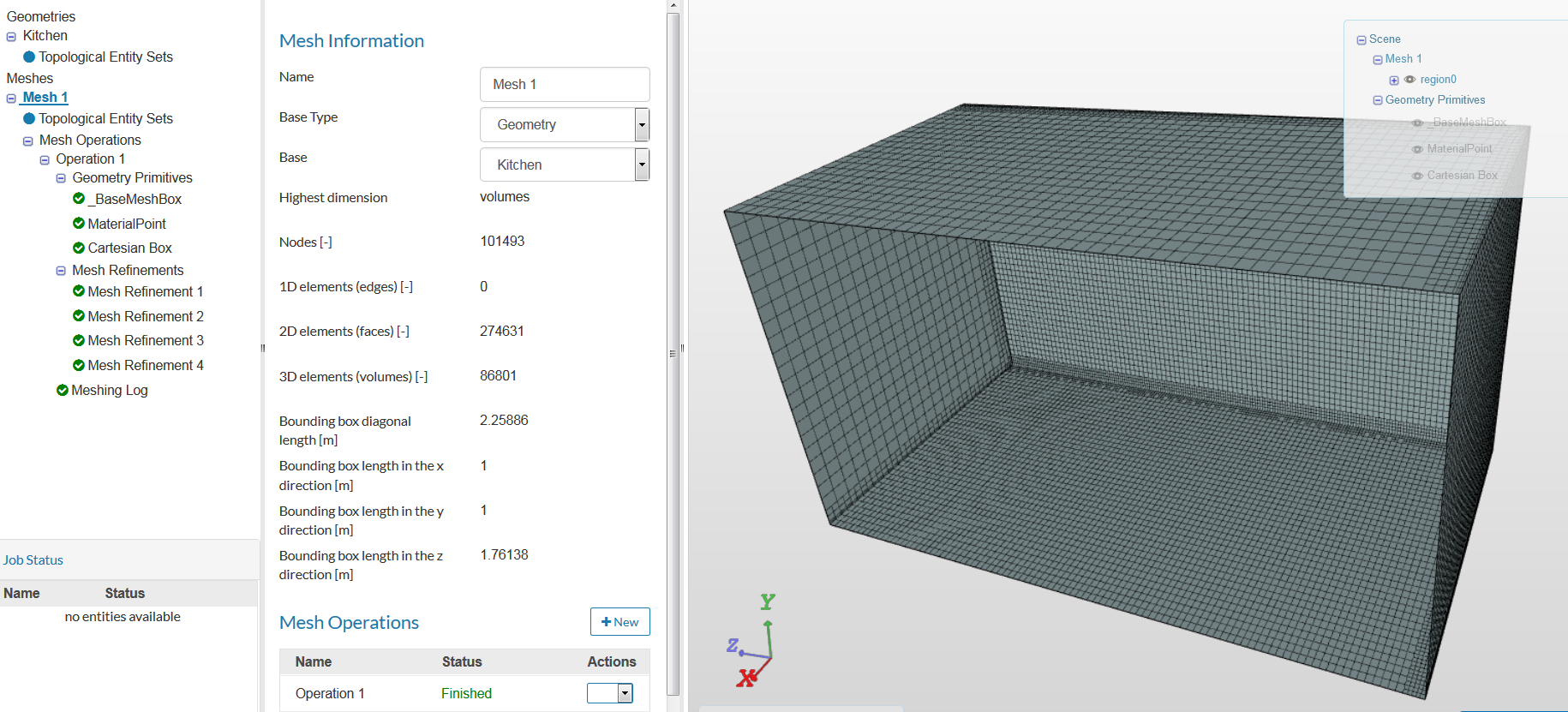
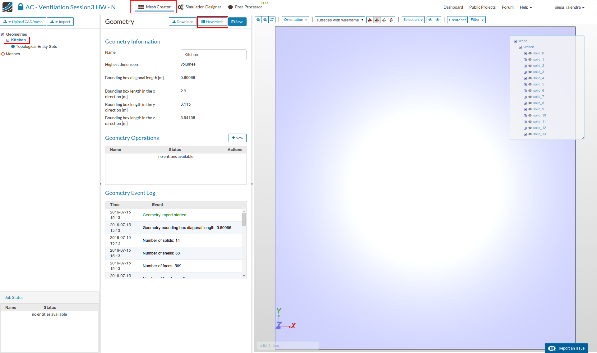
Meshing
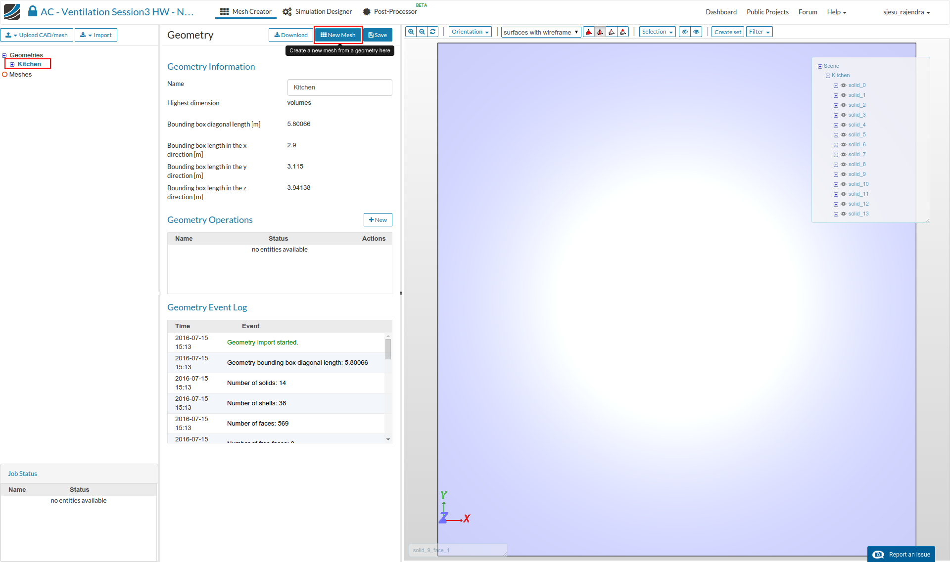
- In the ‘Mesh Creator’ tab, click on the geometry ‘Kitchen’
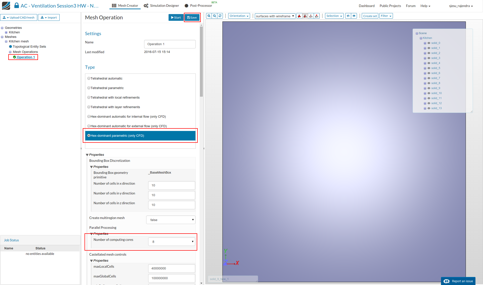
- Then, click on ‘New mesh’ button in the options panel.
- Select the mesh type to be Hex-dominant parametric (only CFD), select the number of cores as 8 and click the Save button.
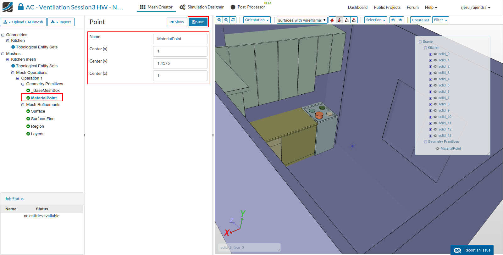
- Click on Material point from the sub-tree and enter the coordinates (1, 1, 1). Click the Save button.
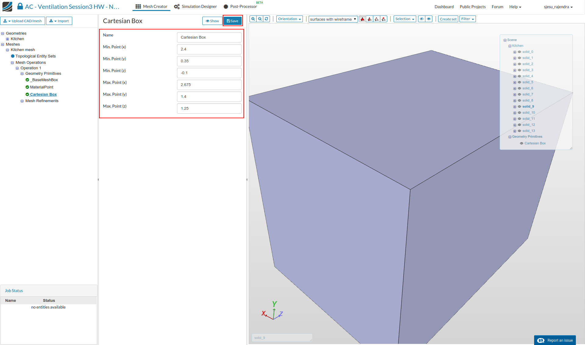
- Click on Geometry primitives and select the New option. Create a new Cartesian box.
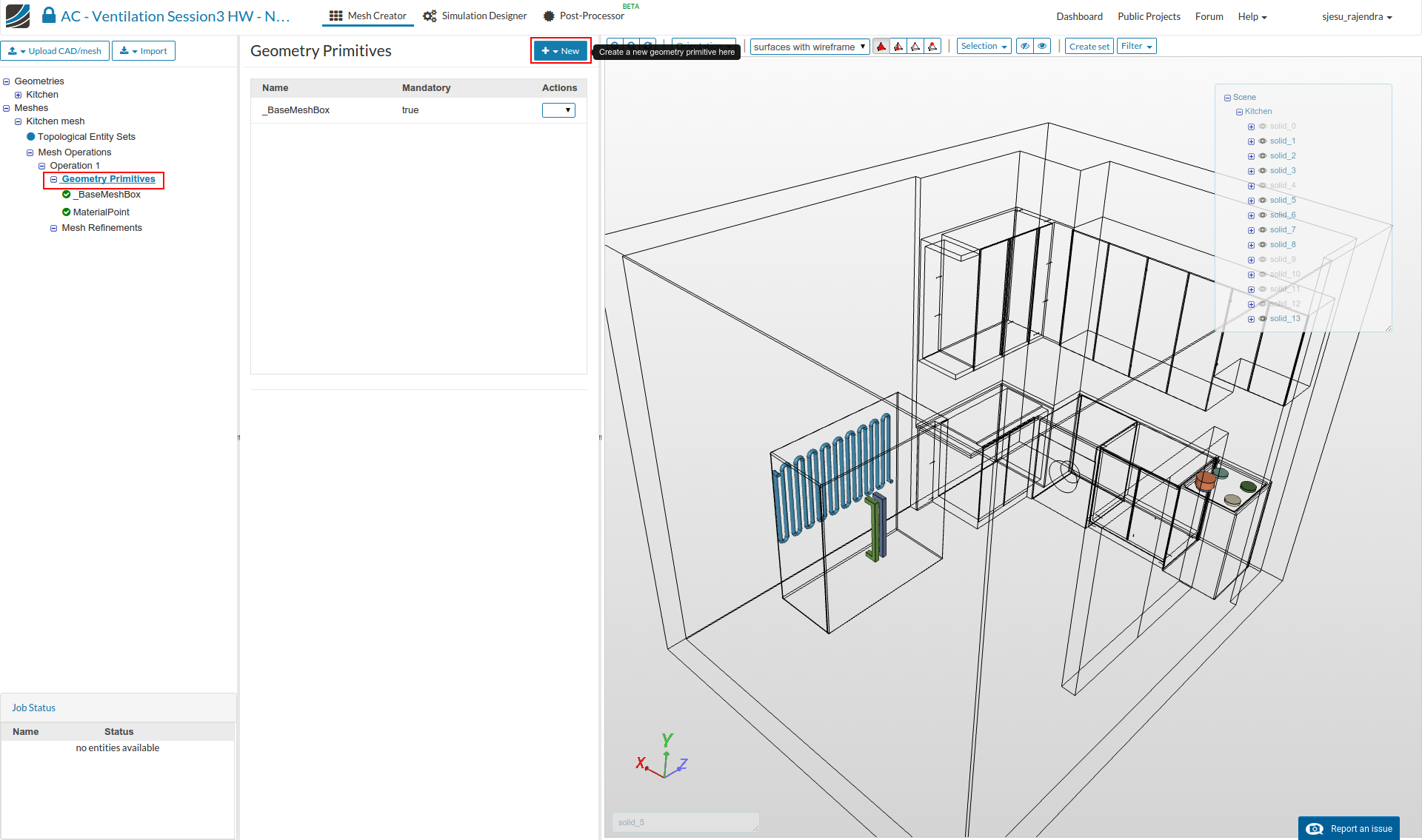
- Enter the following coordinates for the Cartesian box. Minimum coordinates (2.4, 0.35, -0.1) and maximum coordinates (2.675, 1.4, 1.25)
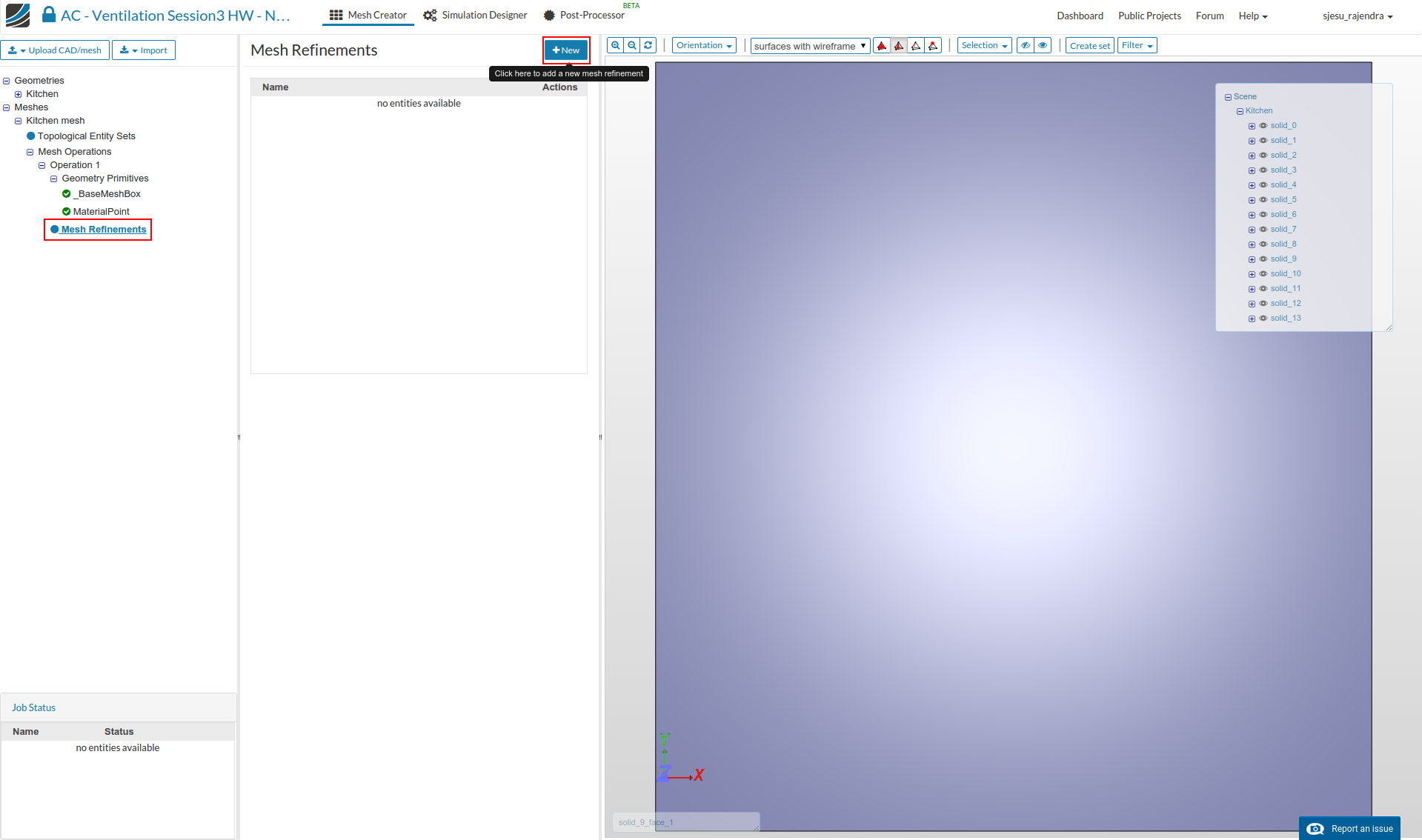
- Click on Mesh refinements and select New button.
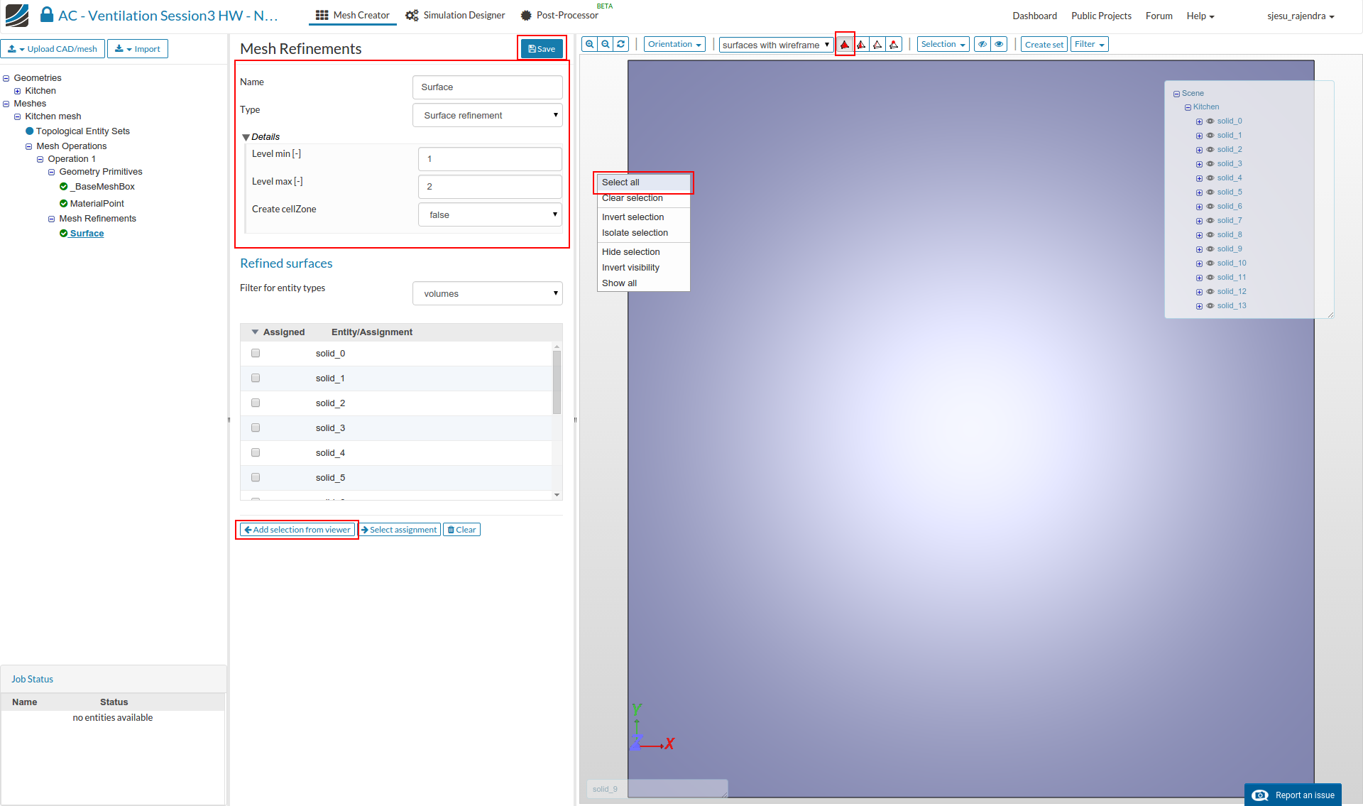
- Create a surface refinement with level 1 to 2 for all the solids. This can be done as shown in the following image. Select ‘Pick solid’ from the pick object toolbar, right click in the viewer and ‘Select all’ entities. Select the Add selection from viewer option and then Save.
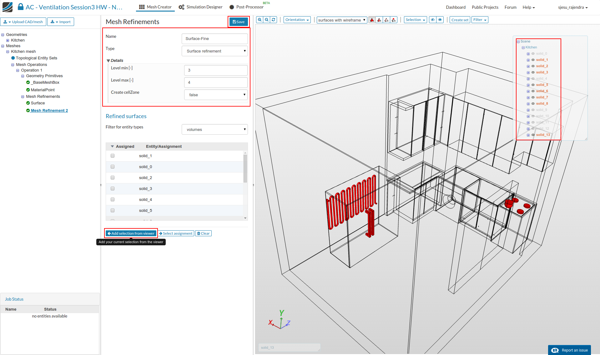
- New fine refinement (level 3 to 4) needs to be created to refine the fine regions. This can be done by selecting the solids (solid_1, solid_2, solid_3, solid_5, solid_6, solid_7, solid_8, solid_13) from the list and then Add selection from viewer. Click the save button.
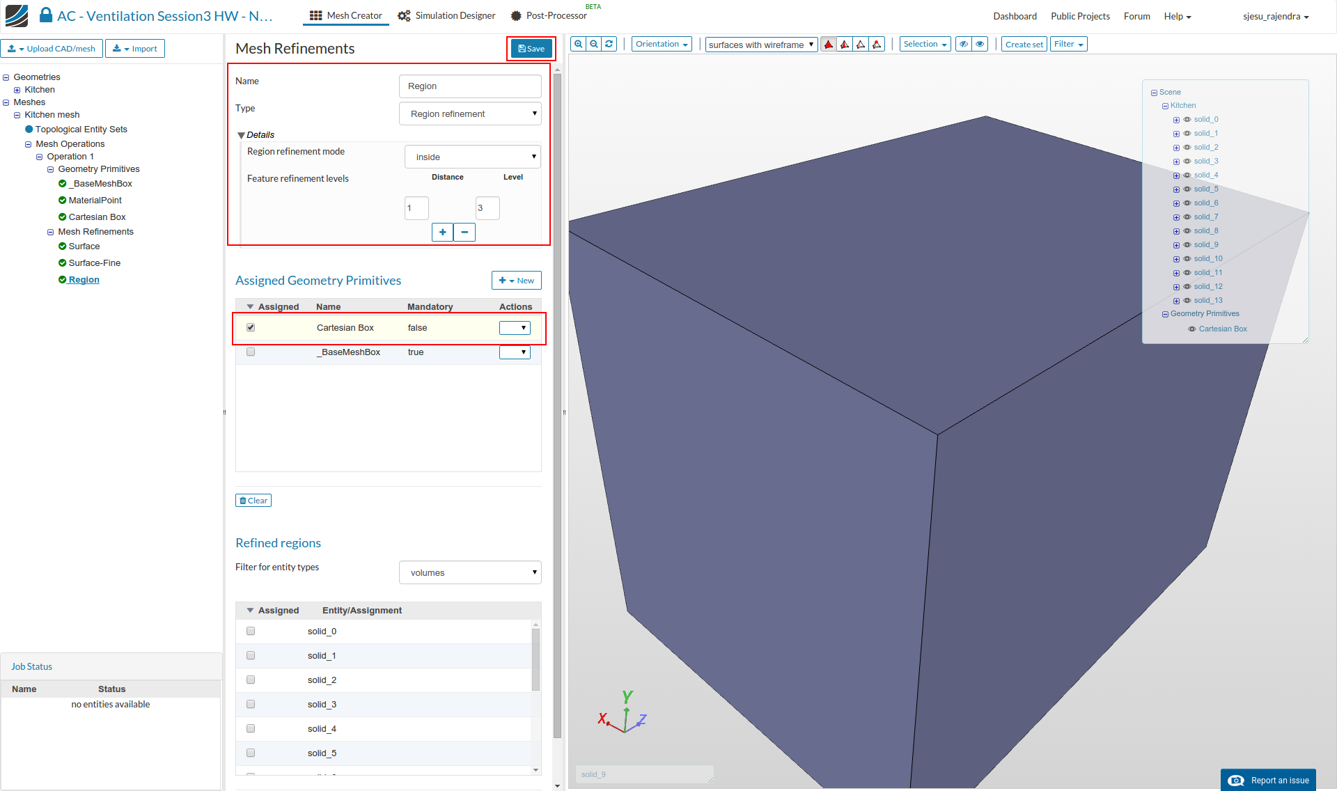
- A region refinement (level 3) is required to get smaller cells near the heat source, i.e. near the refrigerator. This can be done by selecting the ‘Cartesian Box’ from the list of Geometry primitives.
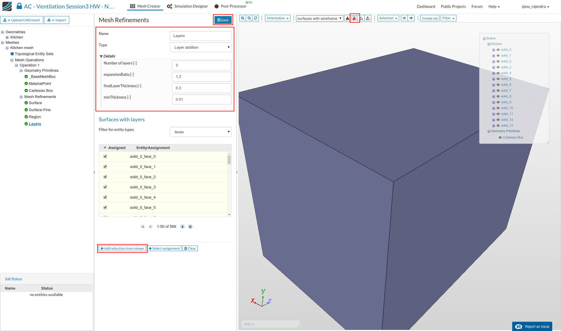
- Finally layers are added to capture the turbulent flow. Switch the selection to ‘Pick surface’ mode, select all surfaces and ‘Add selection from viewer’. Click the ‘Save’ button.
-
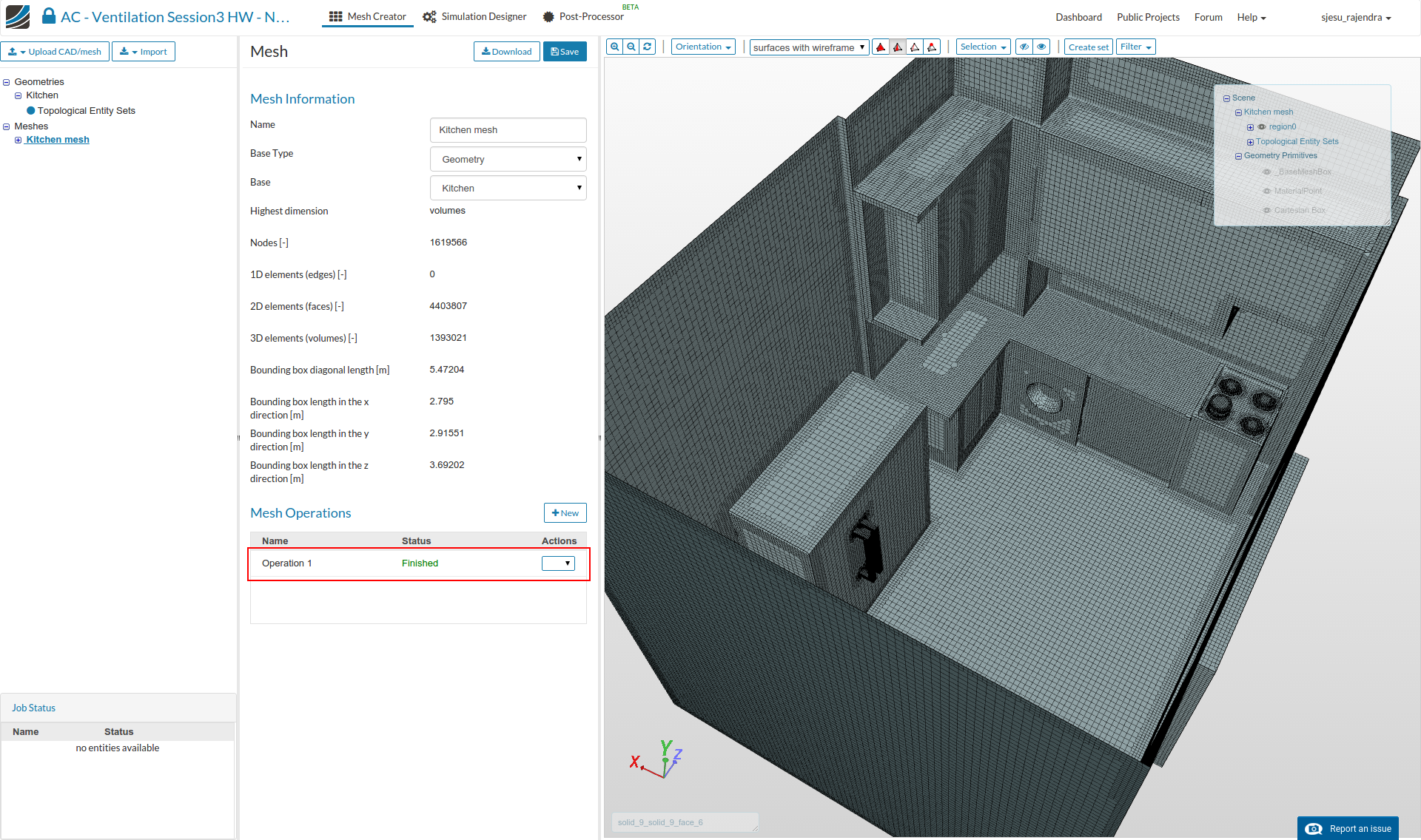
Now click on Operation 1 and select the Start to begin the mesh operation.
-
A message that the mesh operation is finished is seen in the left tab when the mesh generation is complete. It takes approximately 15 minutes for the mesh operation to complete.
Simulation
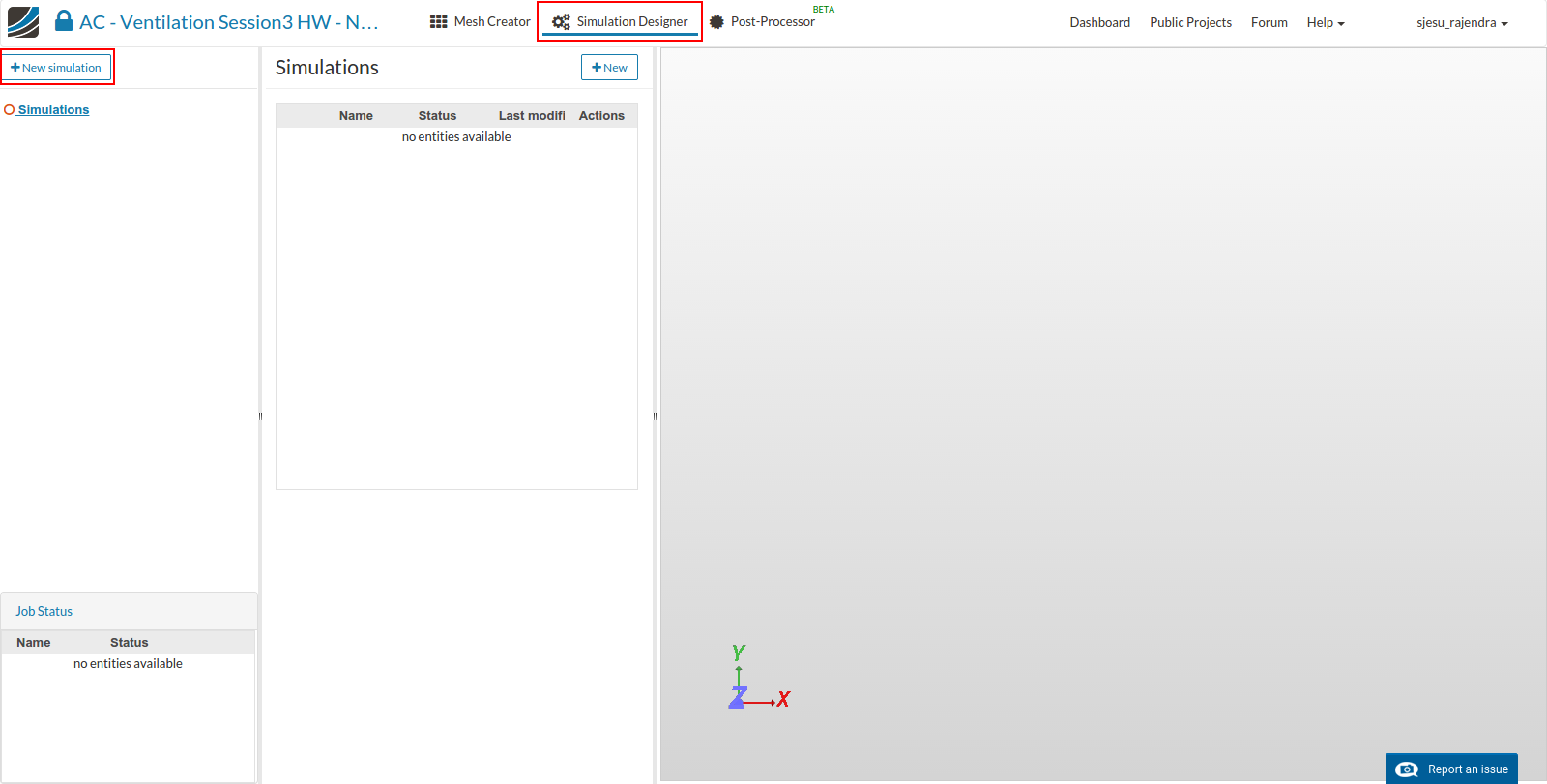
- For setting up the simulation switch to the Simulation Designer tab and select New simulation.
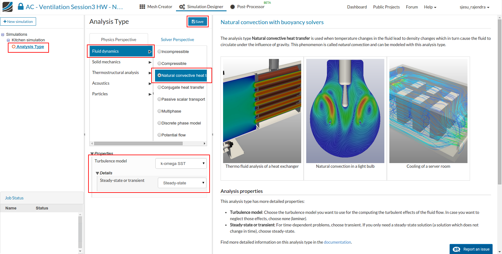
- Change the analysis type to Natural convective heat transfer under Fluid dynamics. Select K-omega SST steady-state type and click Save button.
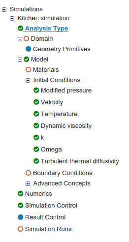
- The simulation tree now looks as shown below.
Selecting domain
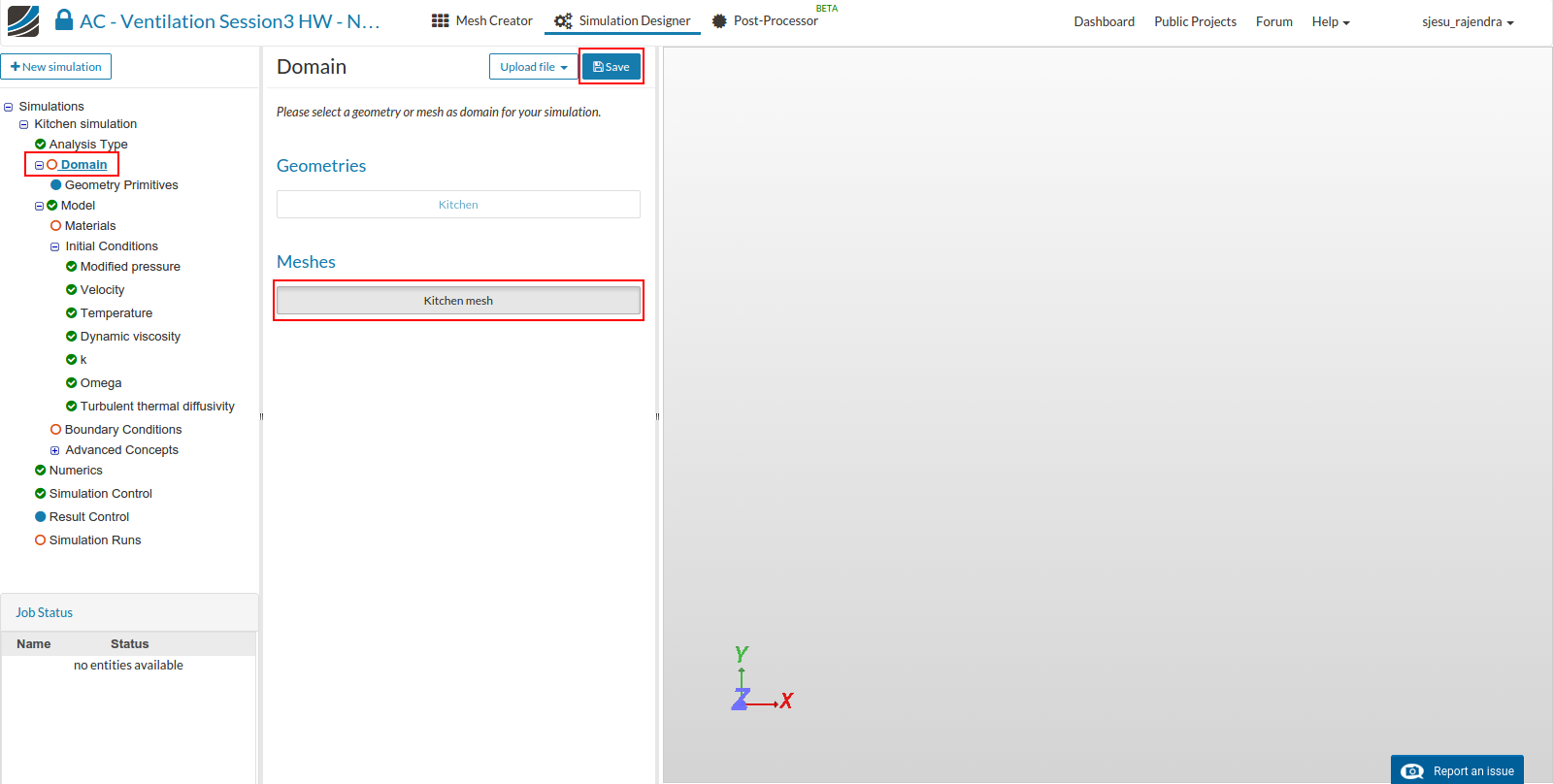
- Click ‘Domain’ from the tree and select the mesh created from the previous task. Click the Save button.
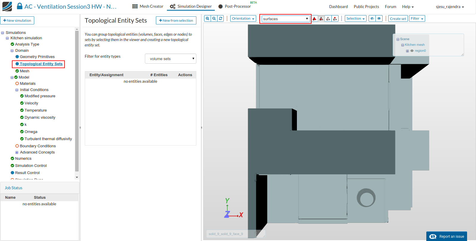
Topological Entity Sets
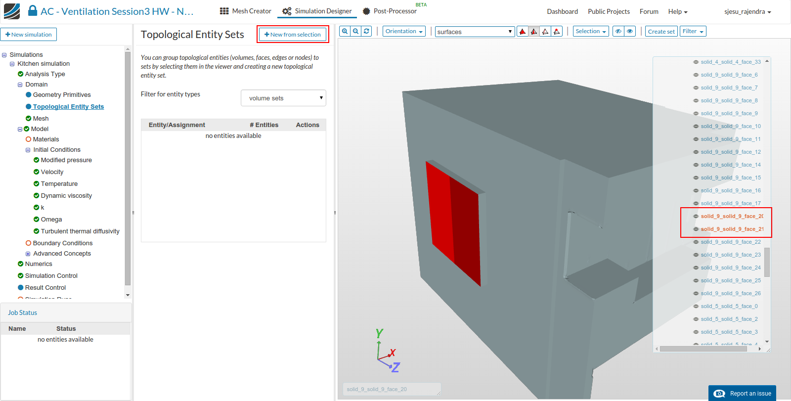
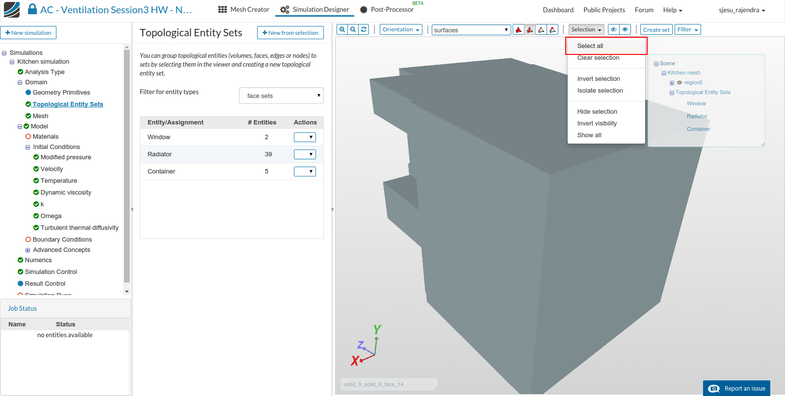
- Click ‘Topological Entity Sets’ to name the different boundary conditions. For better and quick viewing switch the viewer display option to Surfaces.
- Click on the two surfaces (solid_9_solid_9_face_20 and solid_9_solid_9_face_21) as shown in the image and name them as Window by clicking on New from selection.
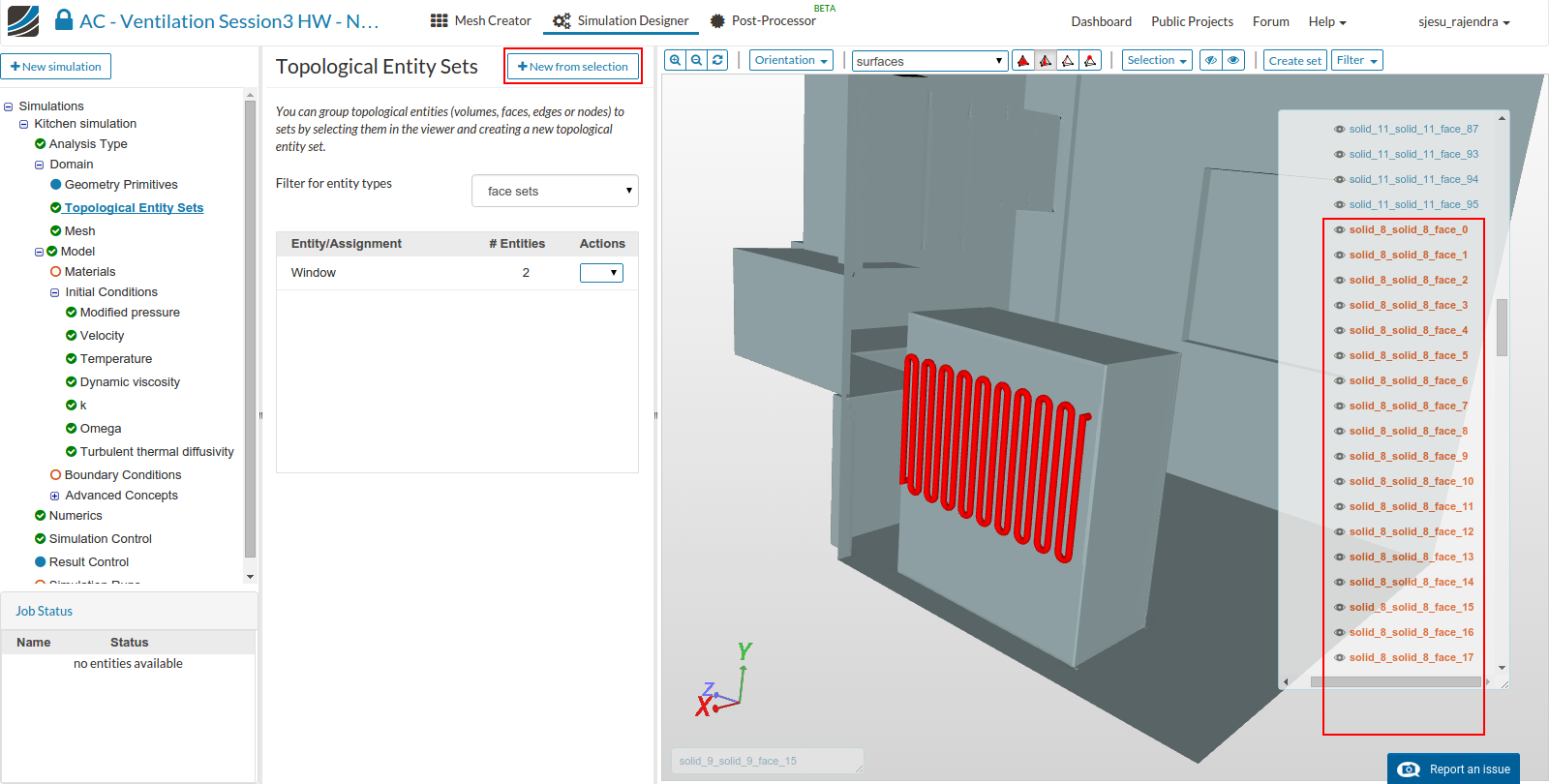
- The selection of refrigerator coil needs to be done manually. This is accomplished by clicking on all the surfaces of solid_8 (solid_8_solid_8_face_0 to solid_8_solid_8_face_39) from the list and click New form selection to name it.
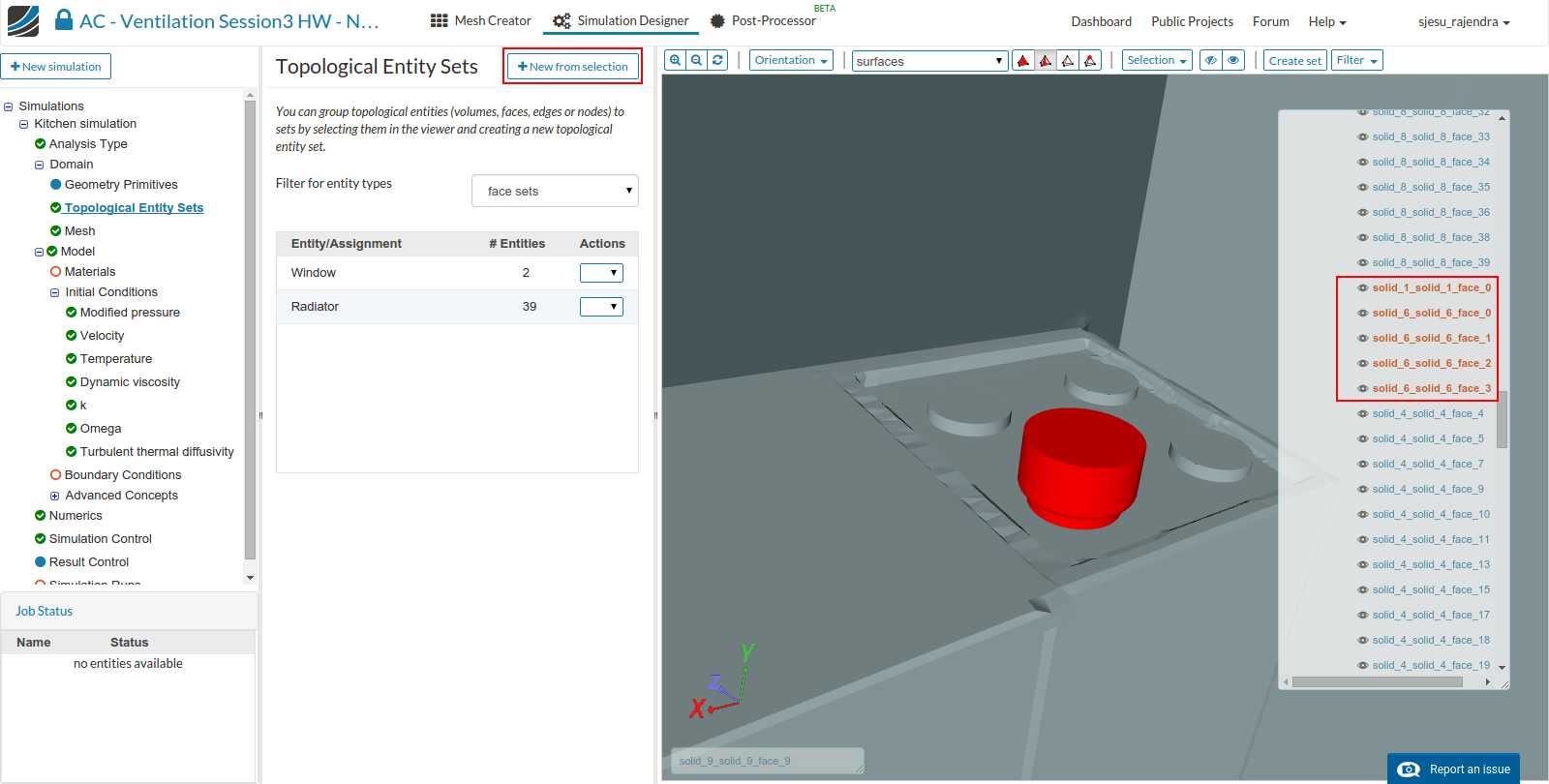
- Now select the container walls to name it. This can be done by selecting the surfaces (solid_1_solid_1_face_0, solid_6_solid_6_face_0, solid_6_solid_6_face_1, solid_6_solid_6_face_2 and solid_6_solid_6_face_3) and clicking New from selection.
- To create a set for the remaining walls, click on each of the entity created and select ‘Hide selection’. Then click on ‘Select all’ form the selection list and select New from selection to create the wall set.
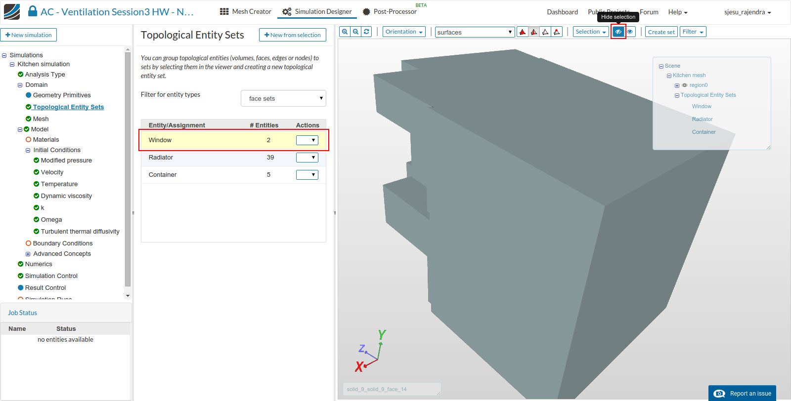
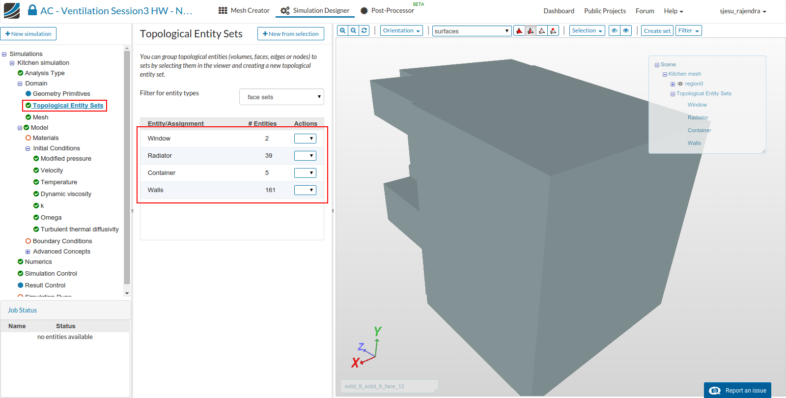
- The final topological entity set looks as follows.
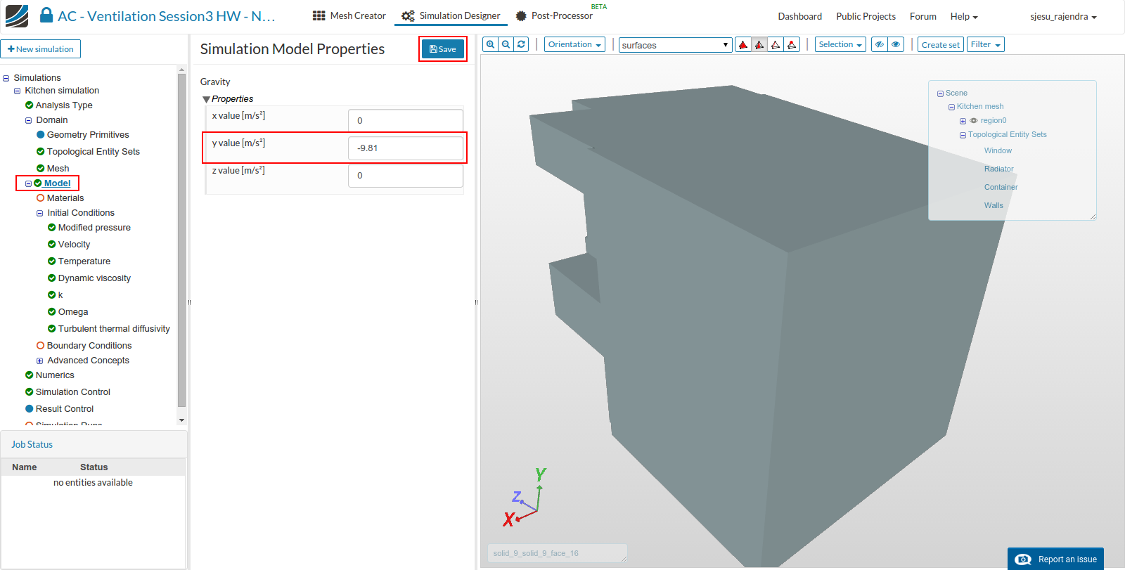
- Click on ‘Model’ and enter gravity value in negative y-direction.
Selecting fluid material
- Select ‘Material’ from the sub-tree and click New.
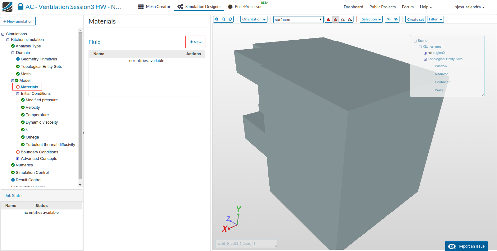
- Select Import from material library.
- Click Air and select the Save button.
- Select region0 from Topological Mapping and click the Save button.
Boundary conditions
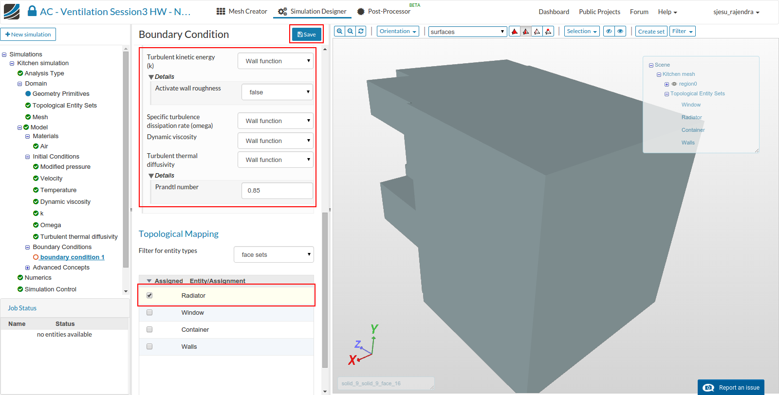
- The initial conditions can be left with the default values. Click on ‘Boundary condition’ and select Add boundary condition.

- Name the boundary condition as Source. Select the Custom type and enter the following properties for velocity (Fixed value of ‘0’), Pressure (Fixed flux pressure), Temperature (Fixed value of 313 K) and turbulence properties (wall functions). Select the entity from Topological Mapping and click Save option.
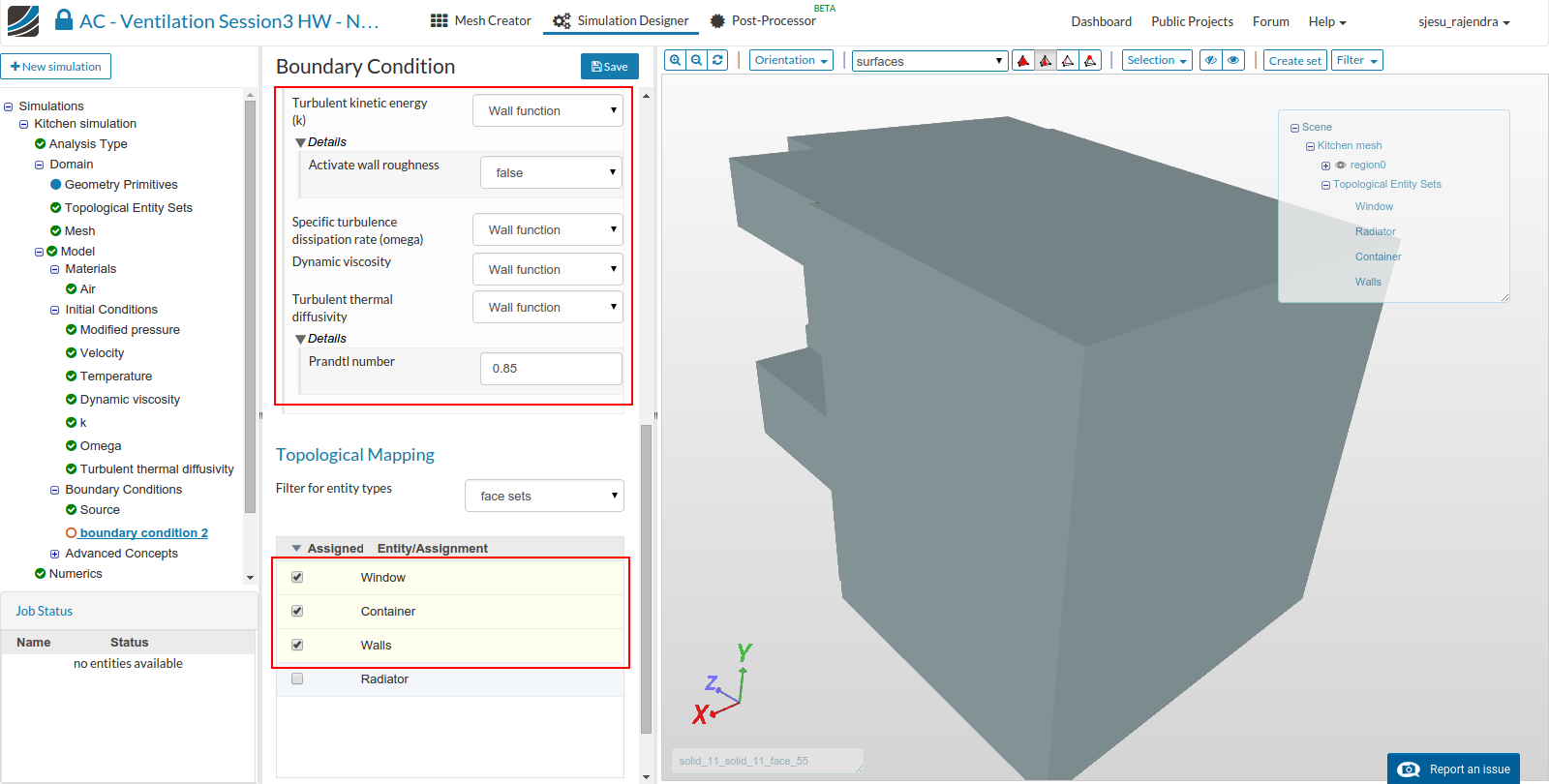
- Add another boundary for Walls. Select the Custom type and enter the following properties for velocity (Fixed value of ‘0’), Pressure (Fixed flux pressure), Temperature (Fixed value of 293 K) and turbulence properties (wall functions). Select the entity from Topological Mapping and click Save option.

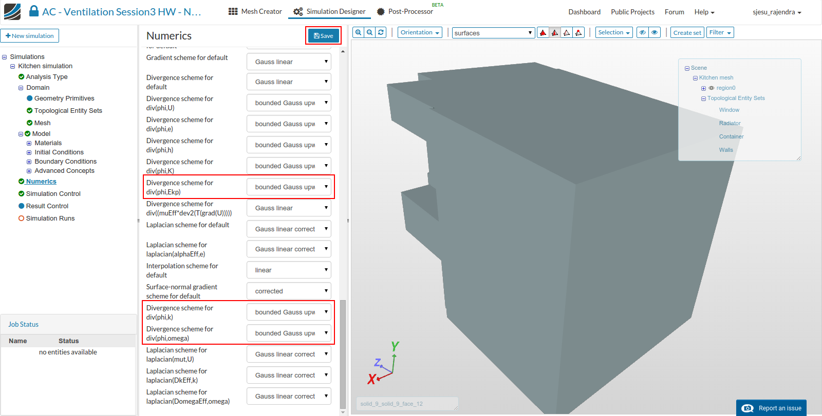
Numerics
- Select ‘Numerics’ from the sub-tree and enter the following values. This enhances us to get the appropriate results.
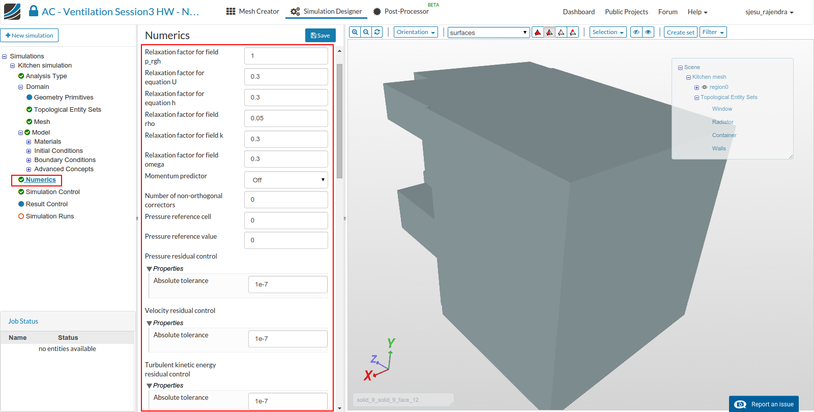
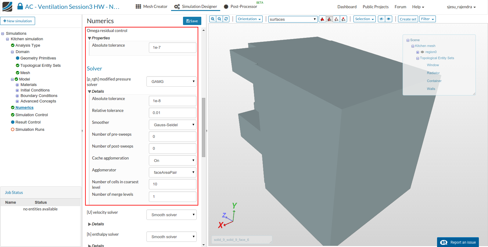
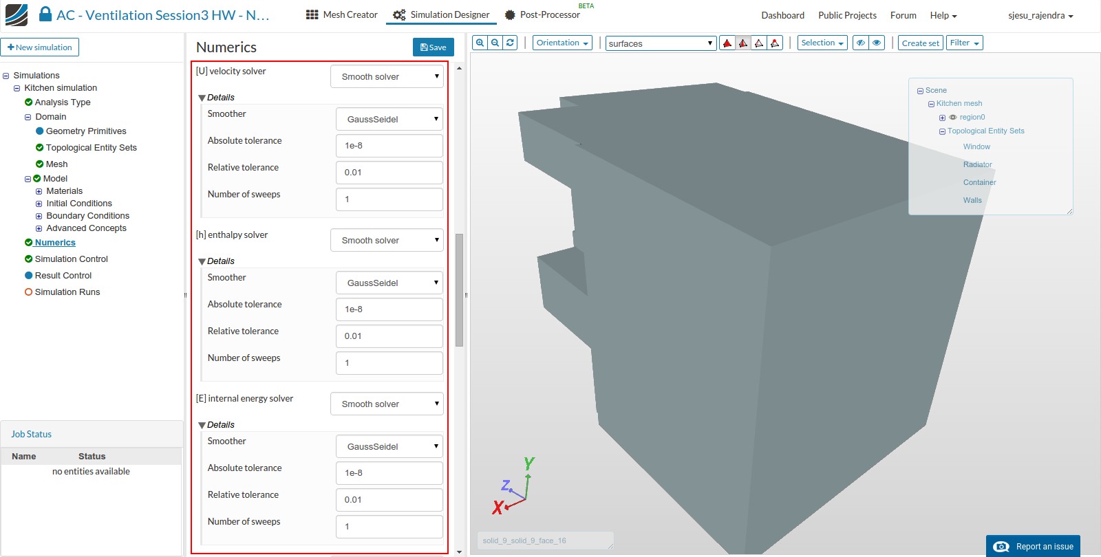
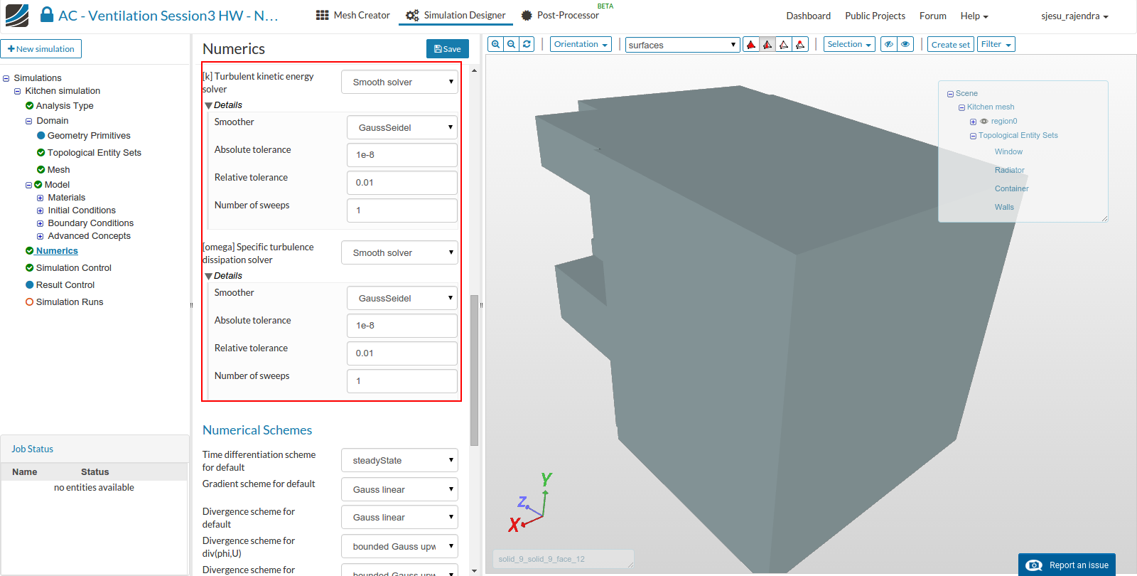
- Finally click the Save button.
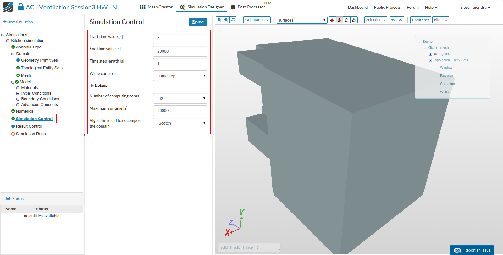
Simulation control
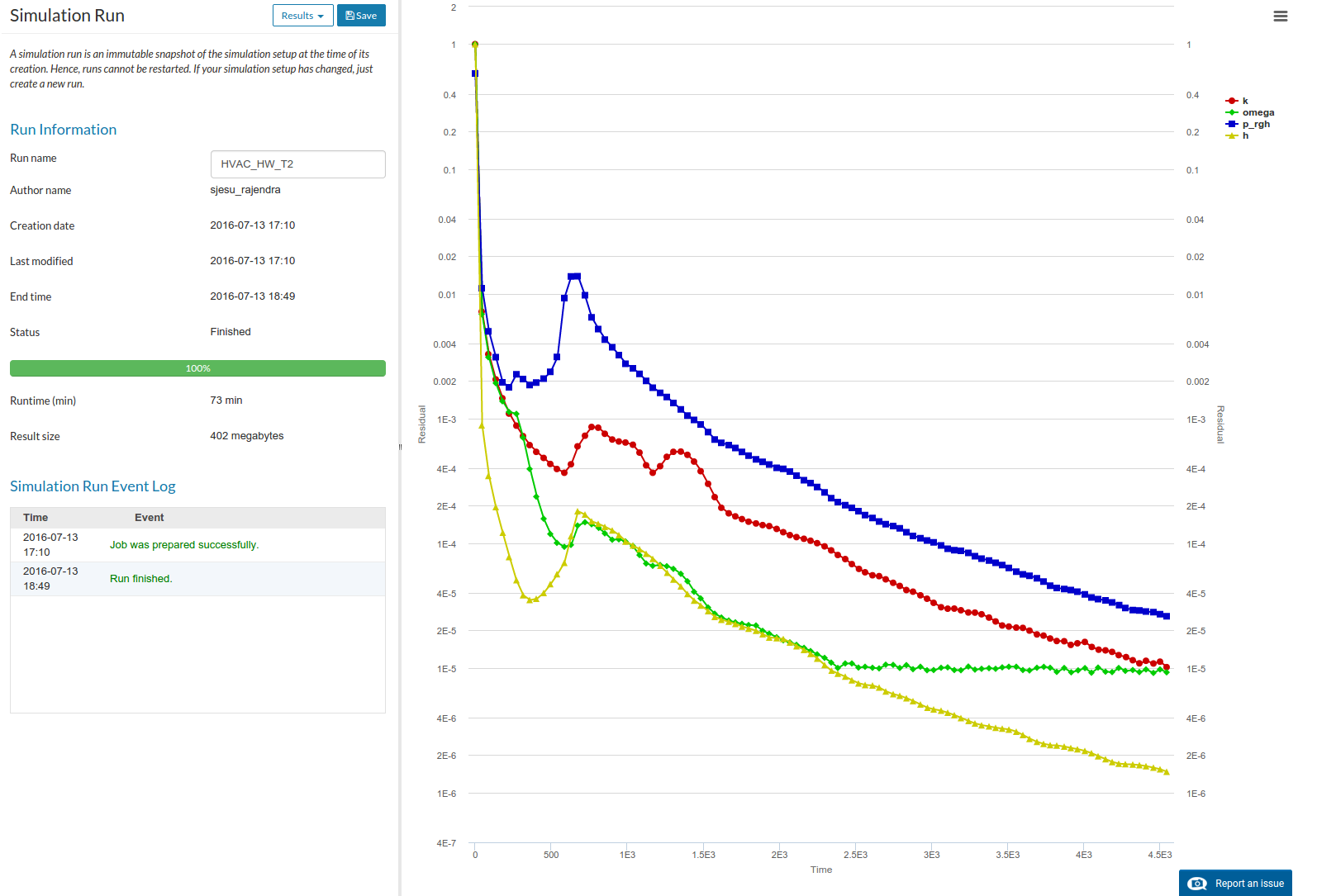
- Click on ‘Simulation control’ and setup the simulation run for 20000s time with a time step of 1.
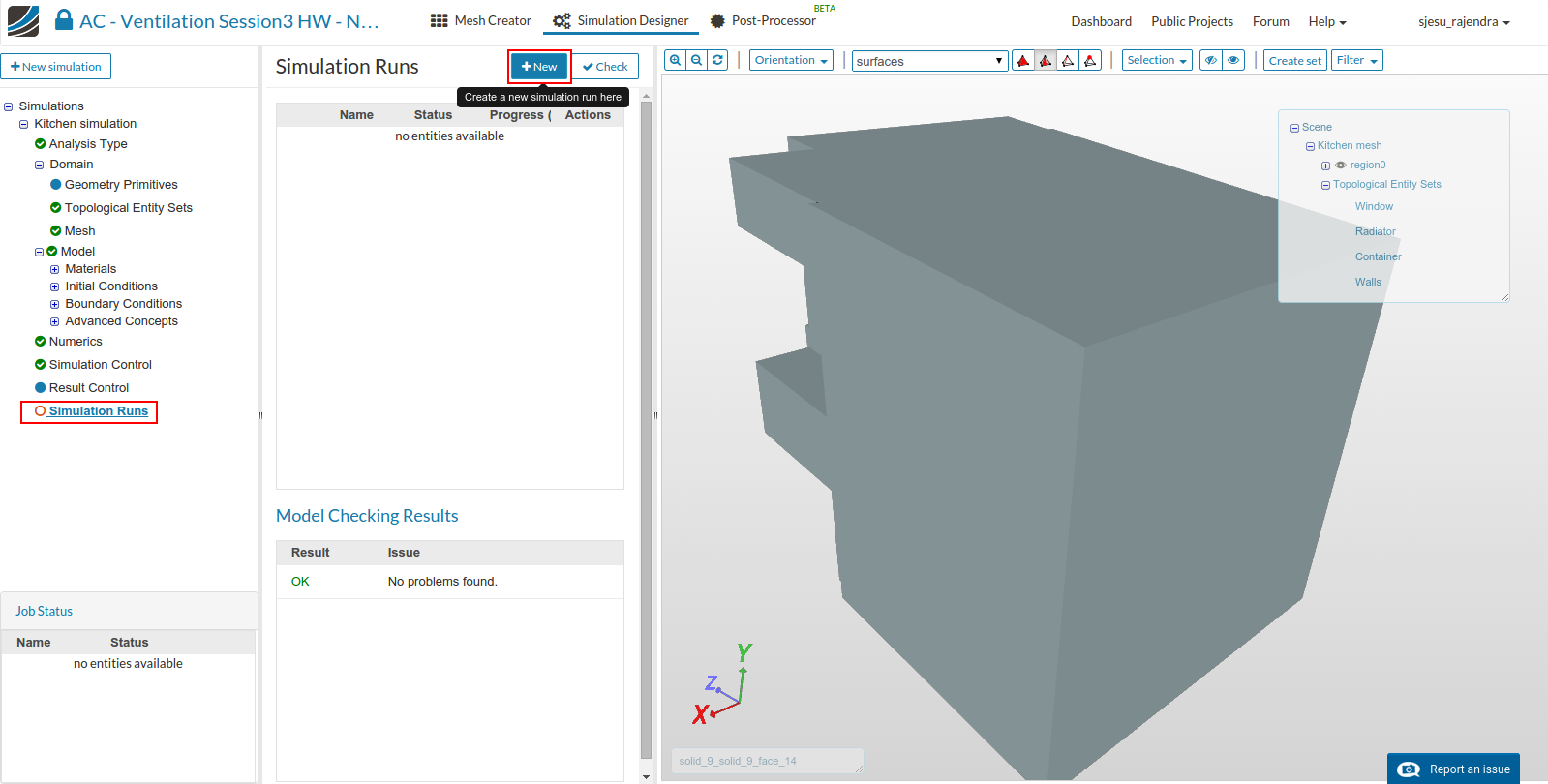
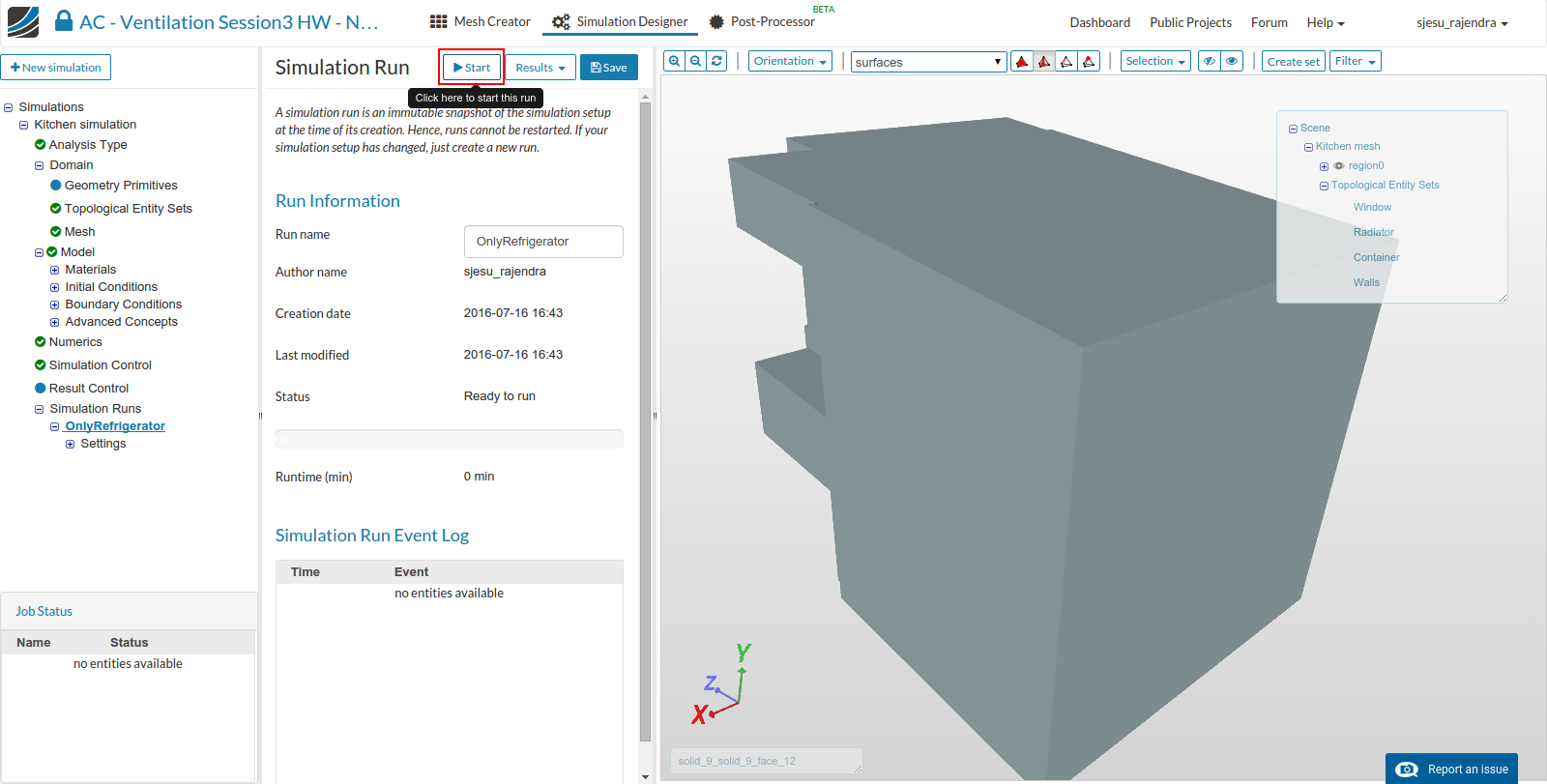
- Select ‘Simulation runs’ and click Create new run. Give it an appropriate name, say ‘Configuration 1’ and press Start button.
Further configurations
- The other 2 configurations can be defined as follows
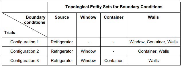
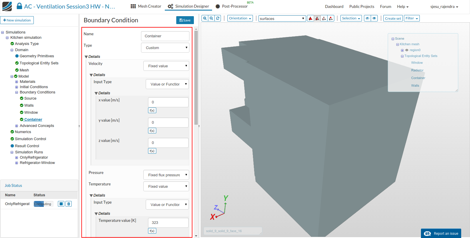
- Similarly create the new simulations, one with window and other with window and container. The boundary conditions of window and container are same as that of wall, except that they are maintained at fixed temperatures of 283 K and 323 K respectively.
Boundary condition for configuration 2

Boundary condition for configuration 3
- Each simulation requires approximately 4 to 5 hours. The simulations can be run in parallel, i.e. you can set up one simulation, then create the next run by changing the boundary conditions.
Post-processing
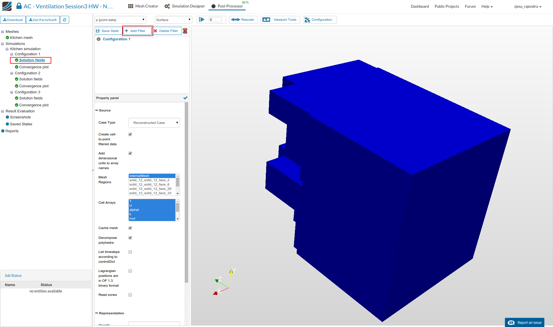
- Once the simulation is over switch to obtain the results by clicking on Post-process results under Results.
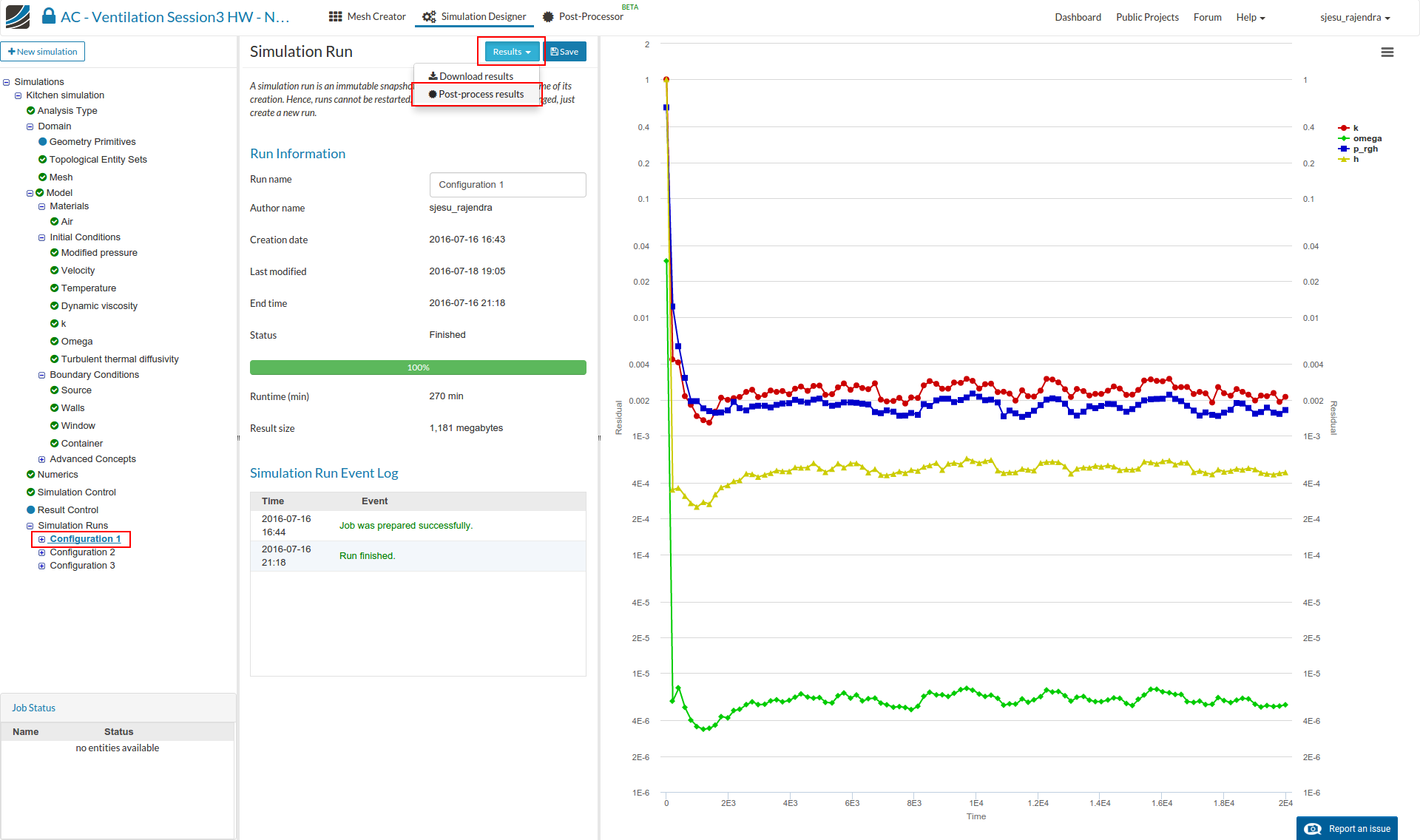
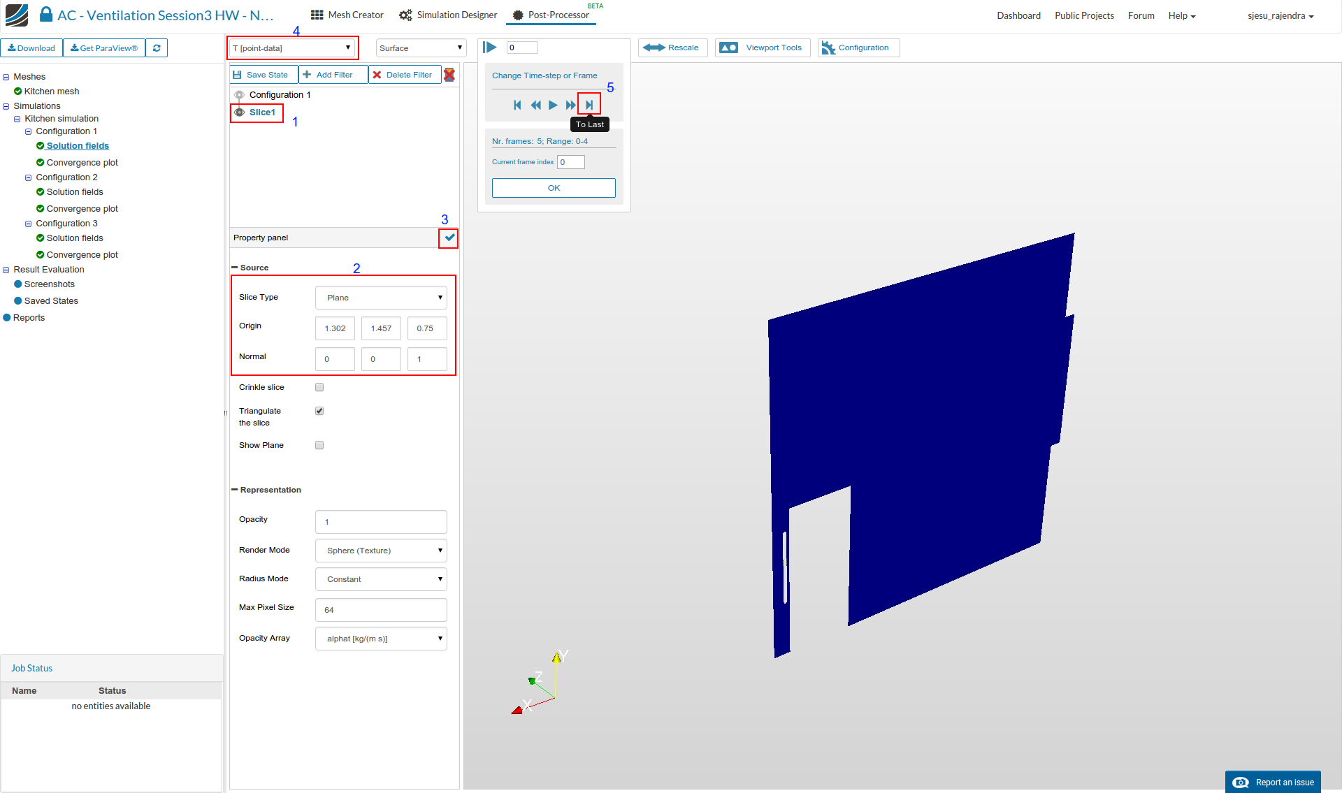
- Click on the solution field (‘Configuration 1’ in this case) and create a slice by clicking Add filter and selecting Slice.
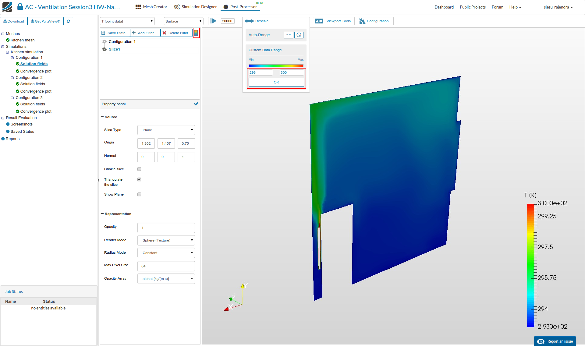
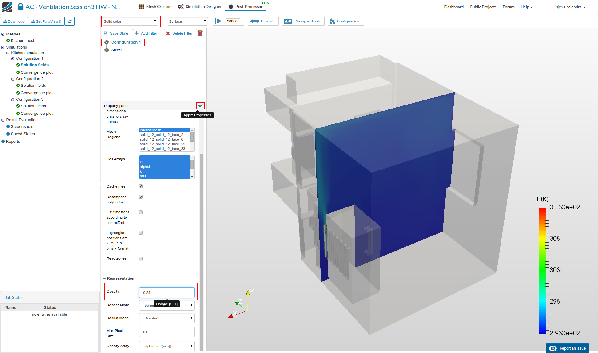
- Enter the values as shown below. Change the data to temperature by selecting T [point-data] and switch results to the last time step.
Slice type - Plane
Origin - (1.302, 1.457, 0.75)
Normal - (0, 0, 1)
- Click the color bar next to filters to show the scale for the value range, and then rescale it between the temperature ranges of 293 K to 300 K.
- It might be interesting to display the domain as well for better visualization. This can be done by changing the opacity to 0.25 and then changing the view property to ‘Solid color’
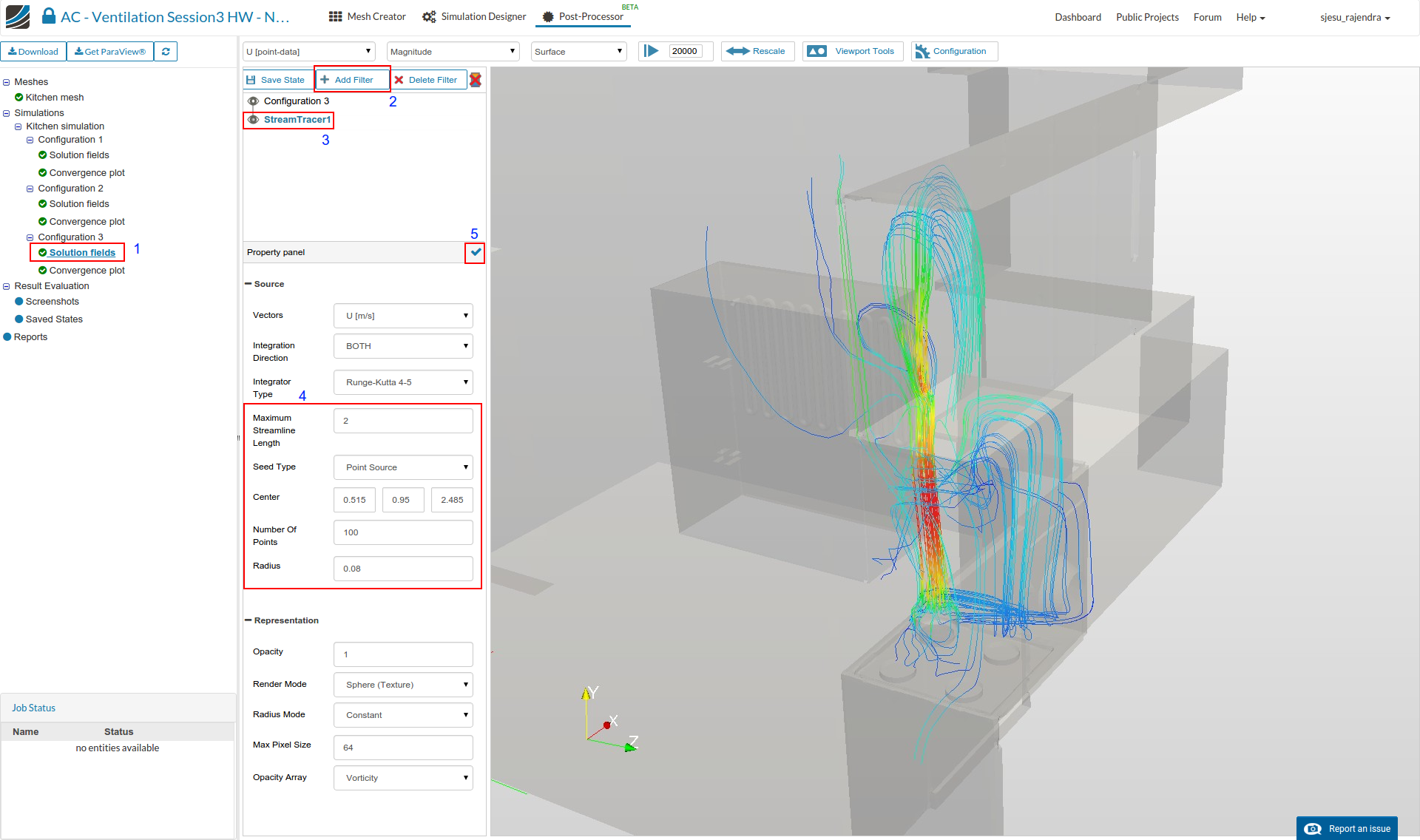
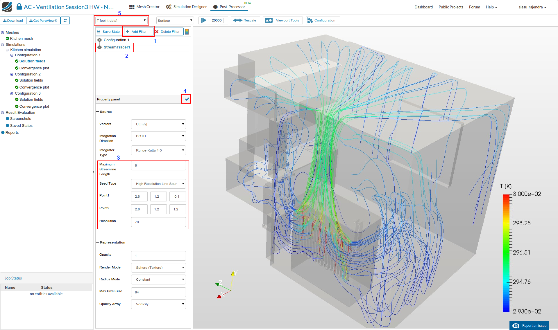
- A stream tracer is created to visualize the flow by adding another filter. Enter the values as shown below.
Maximum streamline length - 6
Seed type - High resolution line source
Point1 - (2.6, 1.2, -0.1)
Point2 - (2.6, 1.2, 1.2)
Resolution - 70
-
For the Configuration 3 which contains the container, a slice can be used to check the temperature distribution around it. This can be done by adding another slice with the following properties.
Slice type - Plane
Origin - (0.5, 1.457, 1.084)
Normal - (1, 0, 0) -
Streamlines can also be added to Configuration 3 for visualizing flow above the container. Add another streamline filter with the following properties.
Maximum streamline length - 2
Seed type - Point source
Center - (0.515, 0.95, 2.485)
Number of points - 100
Radius - 0.08