This post is a continuation of Session-3 Homework and it contains the tutorial to setup the simulation for Aerodynamics of an aircraft.
Simulation Setup
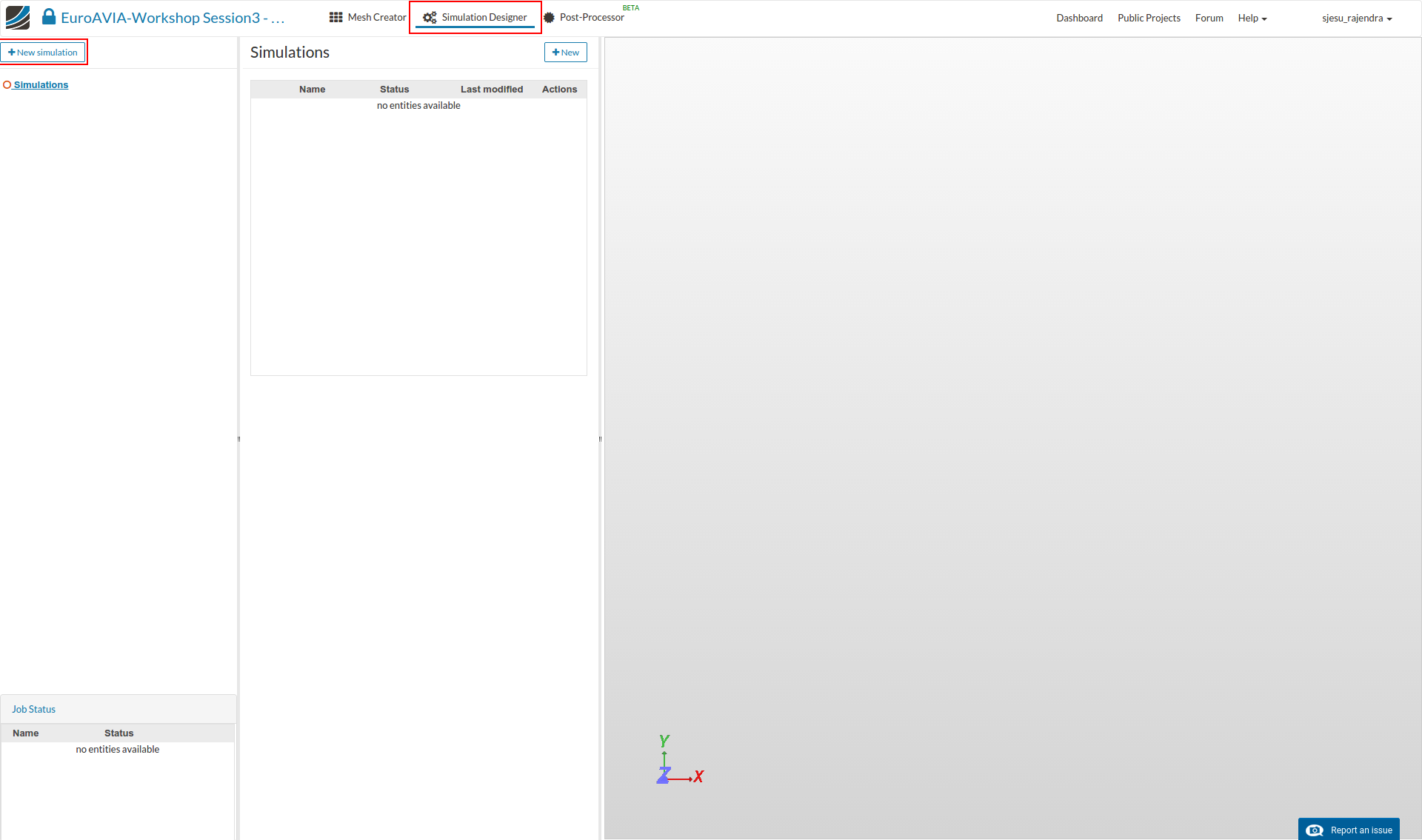
- For setting up the simulation switch to the Simulation Designer tab and select New simulation.
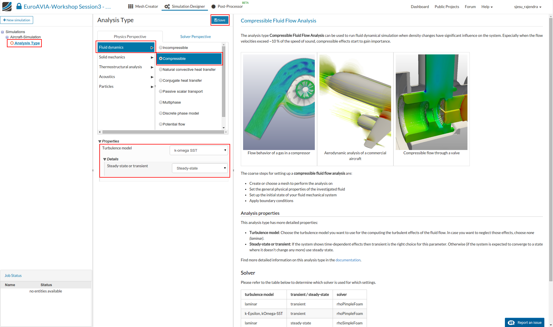
- Select the analysis type: Compressible under Fluid dynamics.
- Select k-omega SST as the turbulence model and Steady-state type and click Save button.
- The flow in aircraft cabin is assumed to be Compressible due to low velocities of the circulated air. Choosing Steady-State option means that we will simulate the Time-Independent solution.
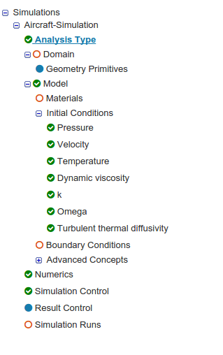
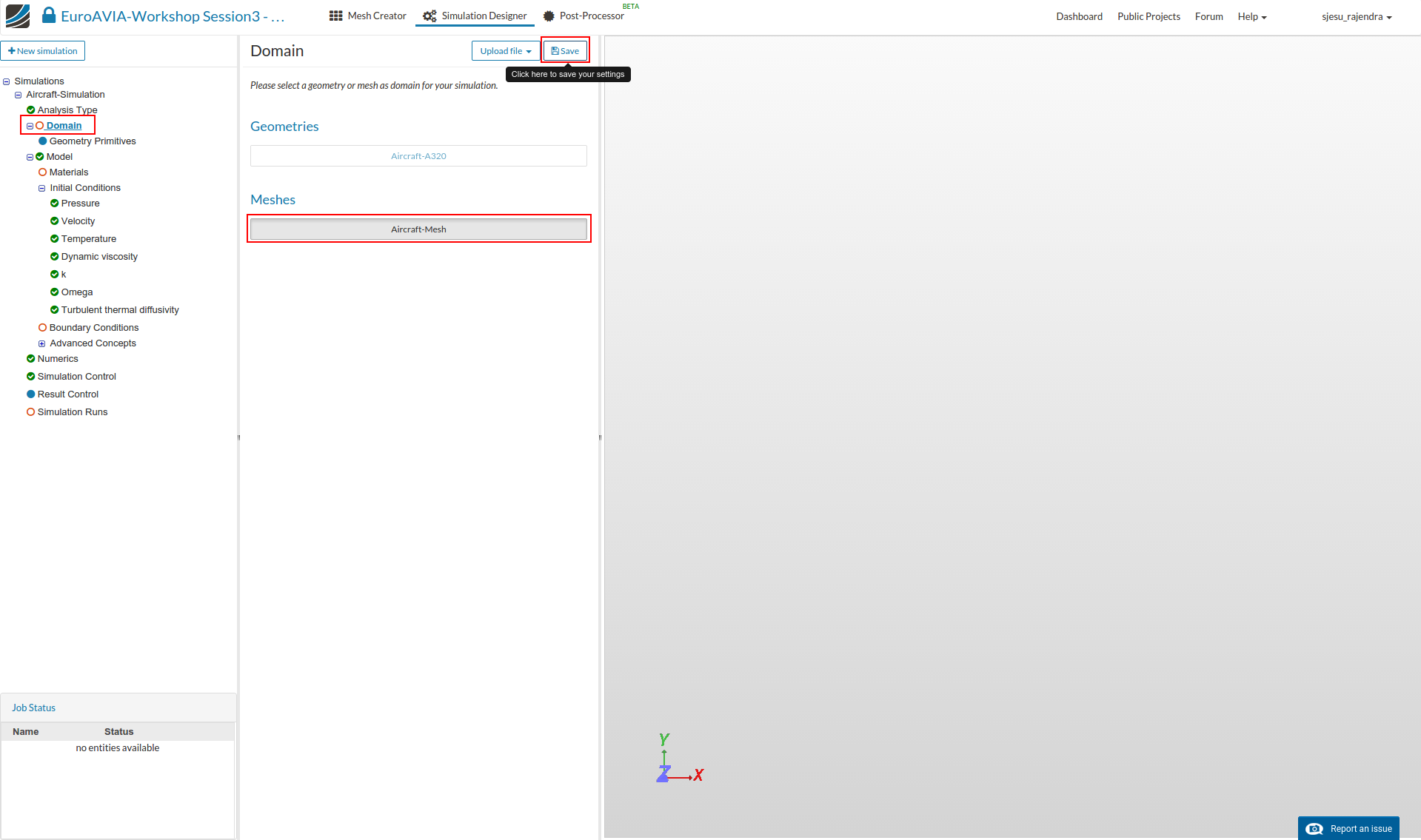
- After saving, the simulation tree now looks as shown below. Here the Tree Entries in Red must be completed.
Domain selection
- Click ‘Domain’ from the tree and select the mesh created from the previous task. Click the Save button. The mesh will then automatically load in the viewer.
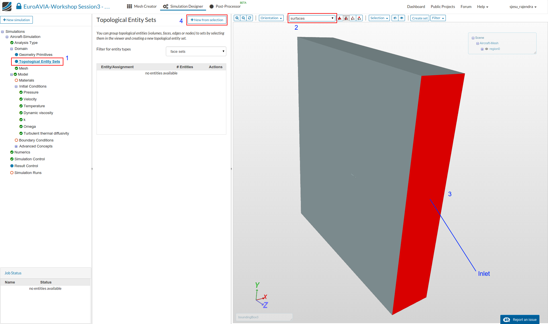
Create Topological Entity Sets
- Click on the tree entry ‘Topological Entity Sets’. Switch to Surface view so that the viewer loads faster.
Inlet:
- To create the first set, click the shown surface (such that the inlet velocity is given in the negative-Z direction) and click on the ‘New from selection’ button to create a set named ‘Inlet’.
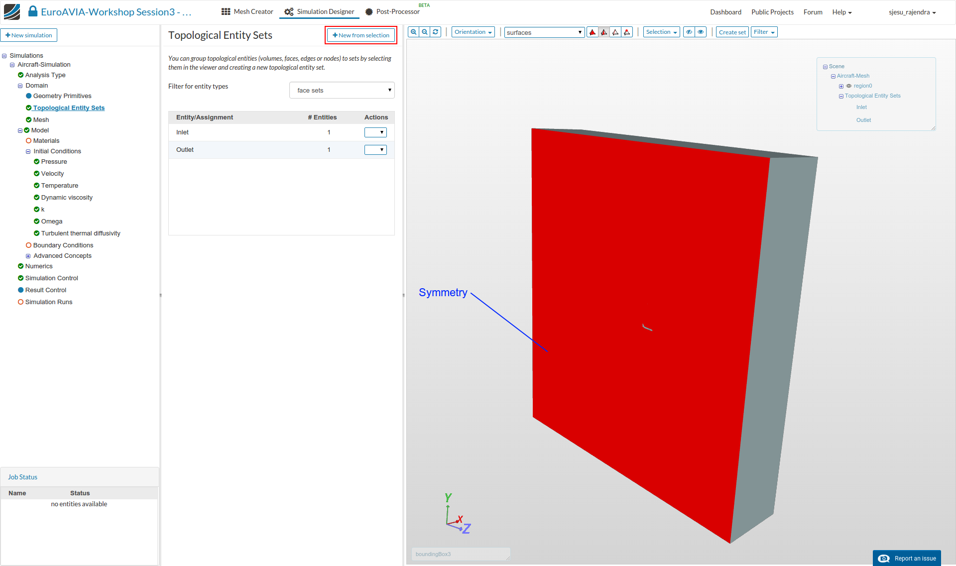
Outlet:
- Similarly, select the shown surface and create a new set named ‘Outlet’.

Symmetry:
- The face shown below is selected for defining the ‘Symmetry’ condition
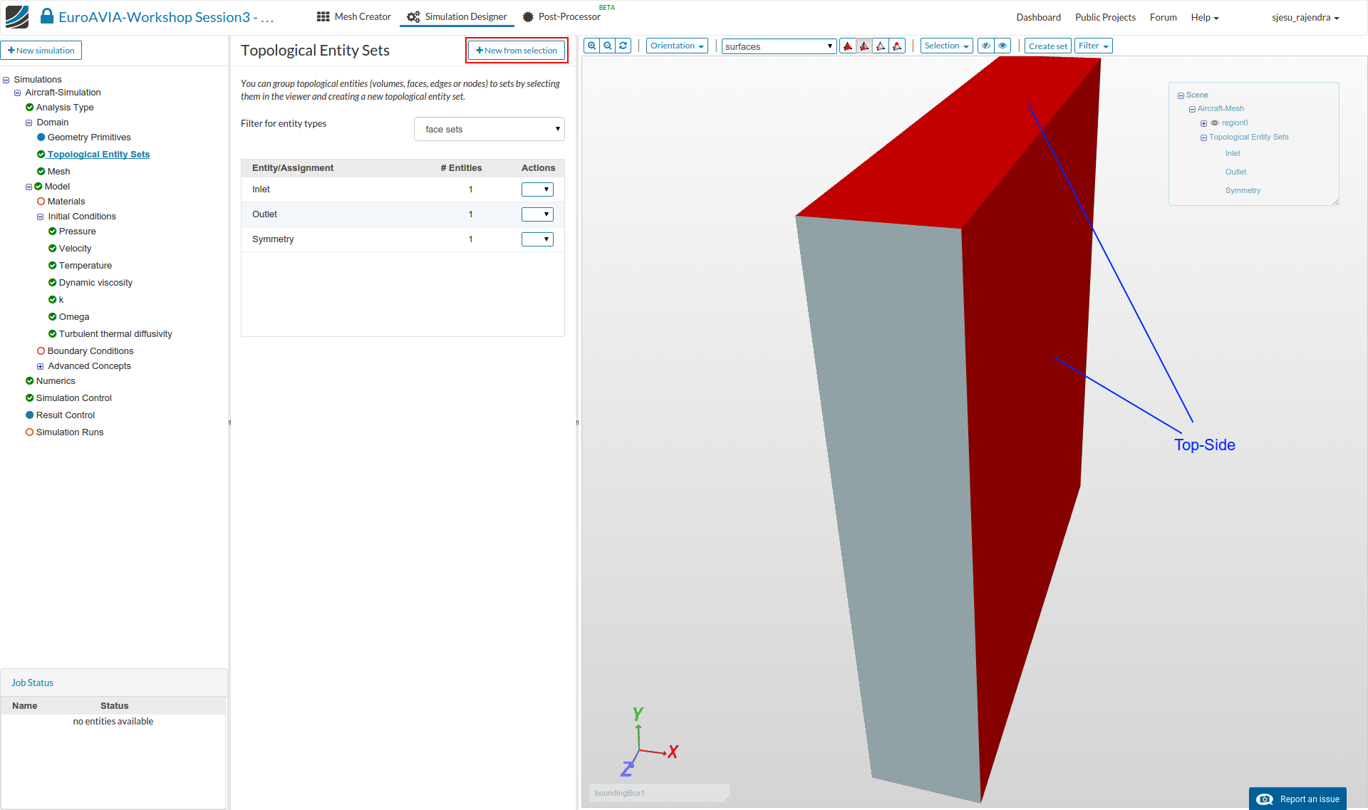
Top and side walls:
- The top and side walls are to be defined similar boundary conditions. Hence they are named as a single entity ‘Top-Side’.
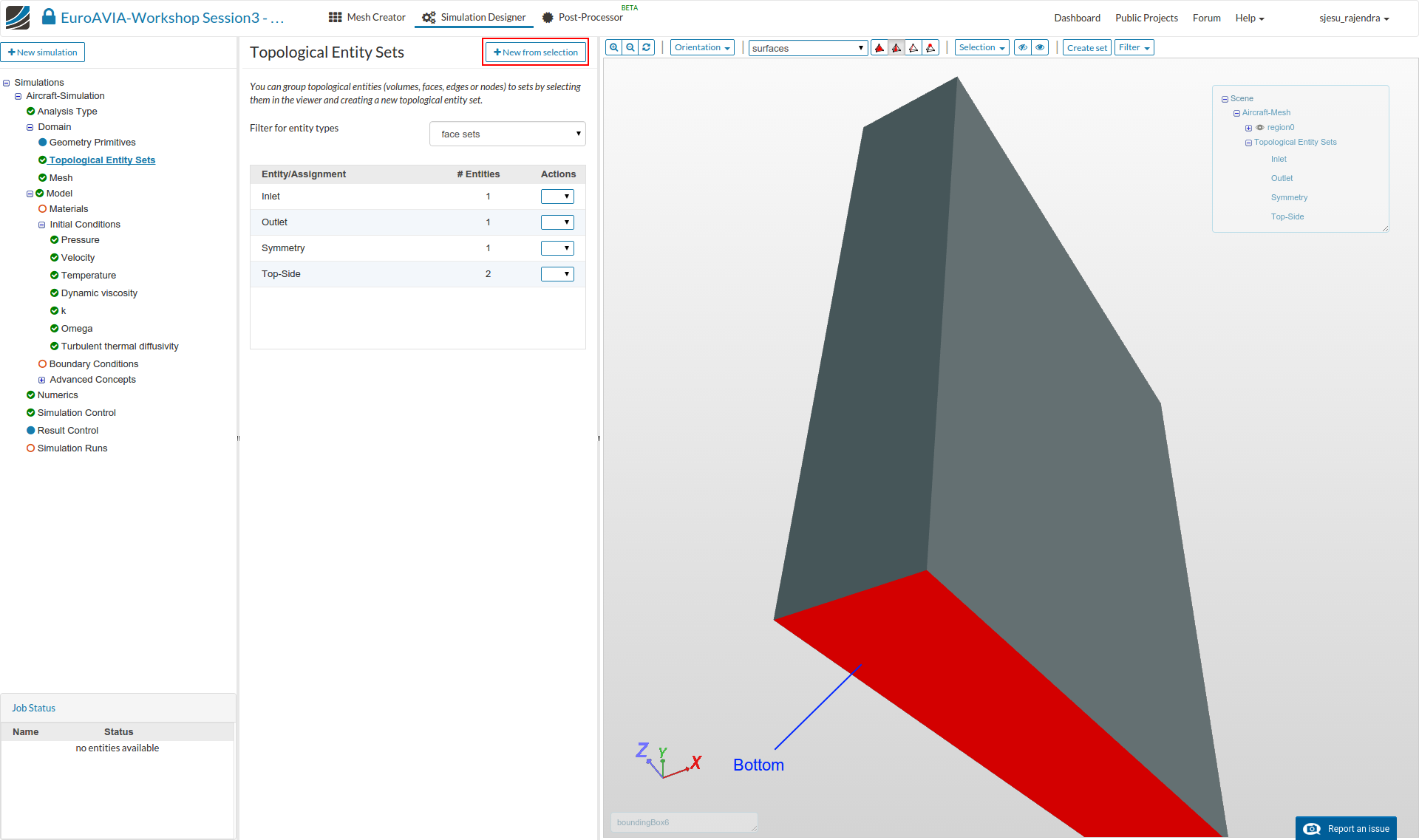
Bottom wall:
- The bottom face is selected and named as ‘Bottom’
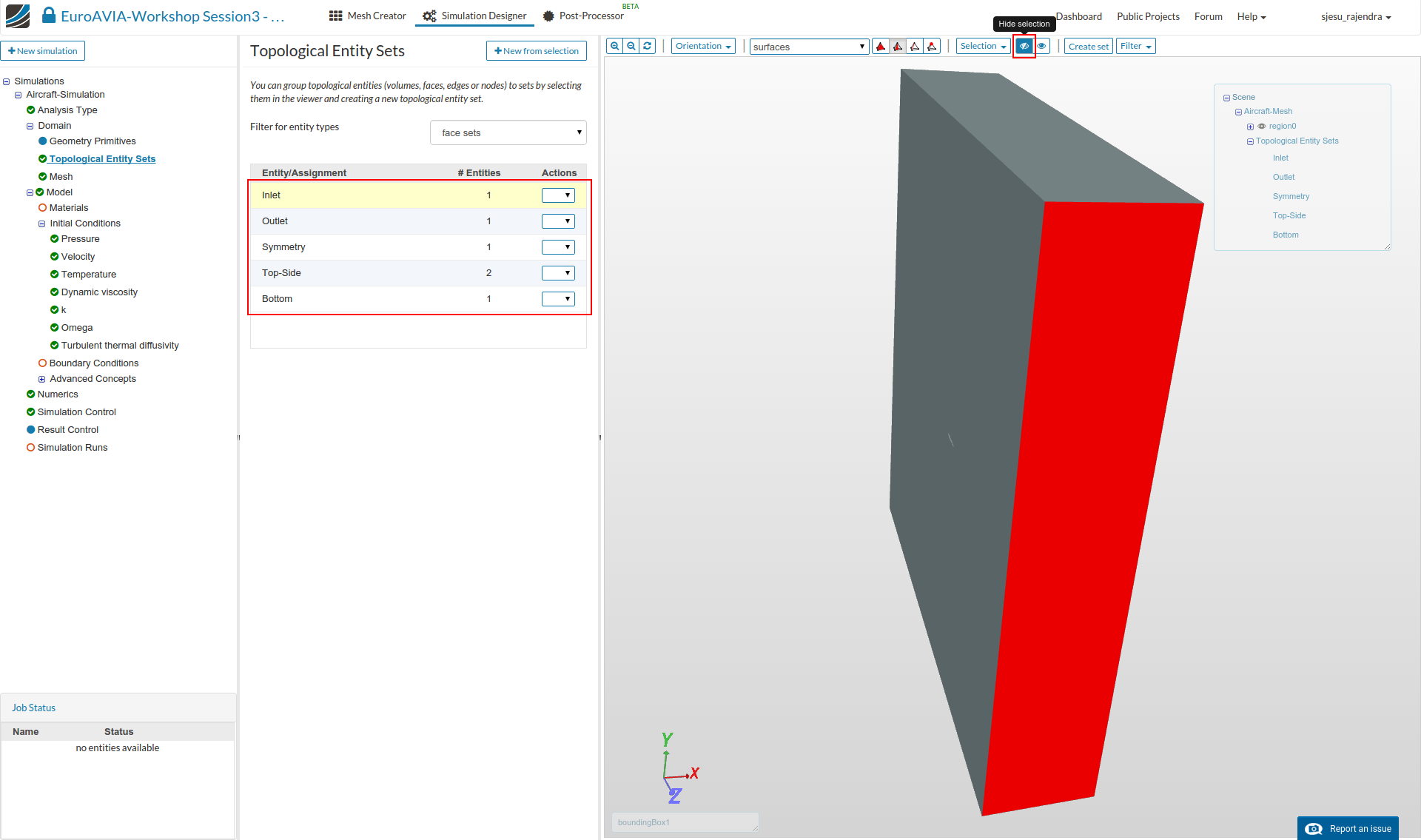
Aircraft - Walls:
- The boundary faces of the aircraft needs to be assigned a name. Hence we select each of the named entity and hide the selection.
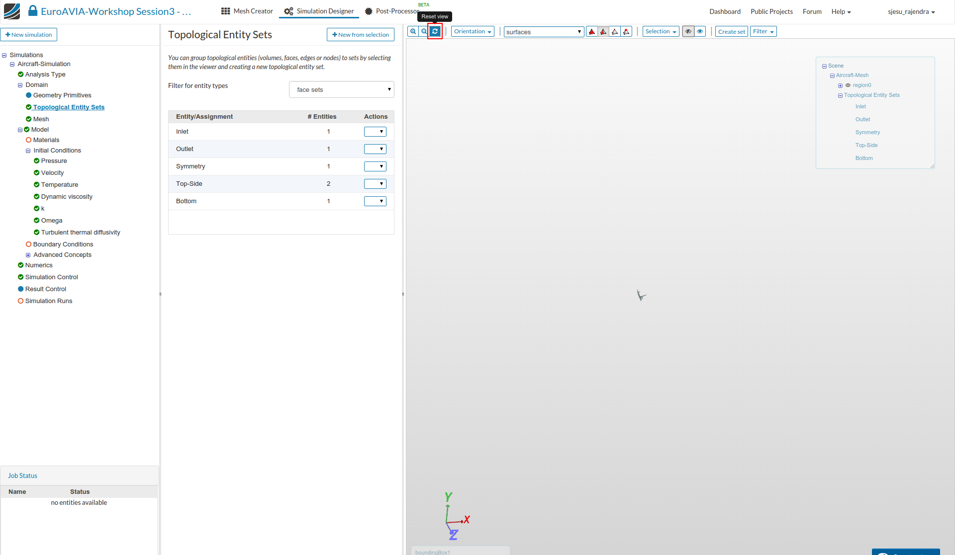
- We can reset the view to fit to screen to see the faces which are not hidden.
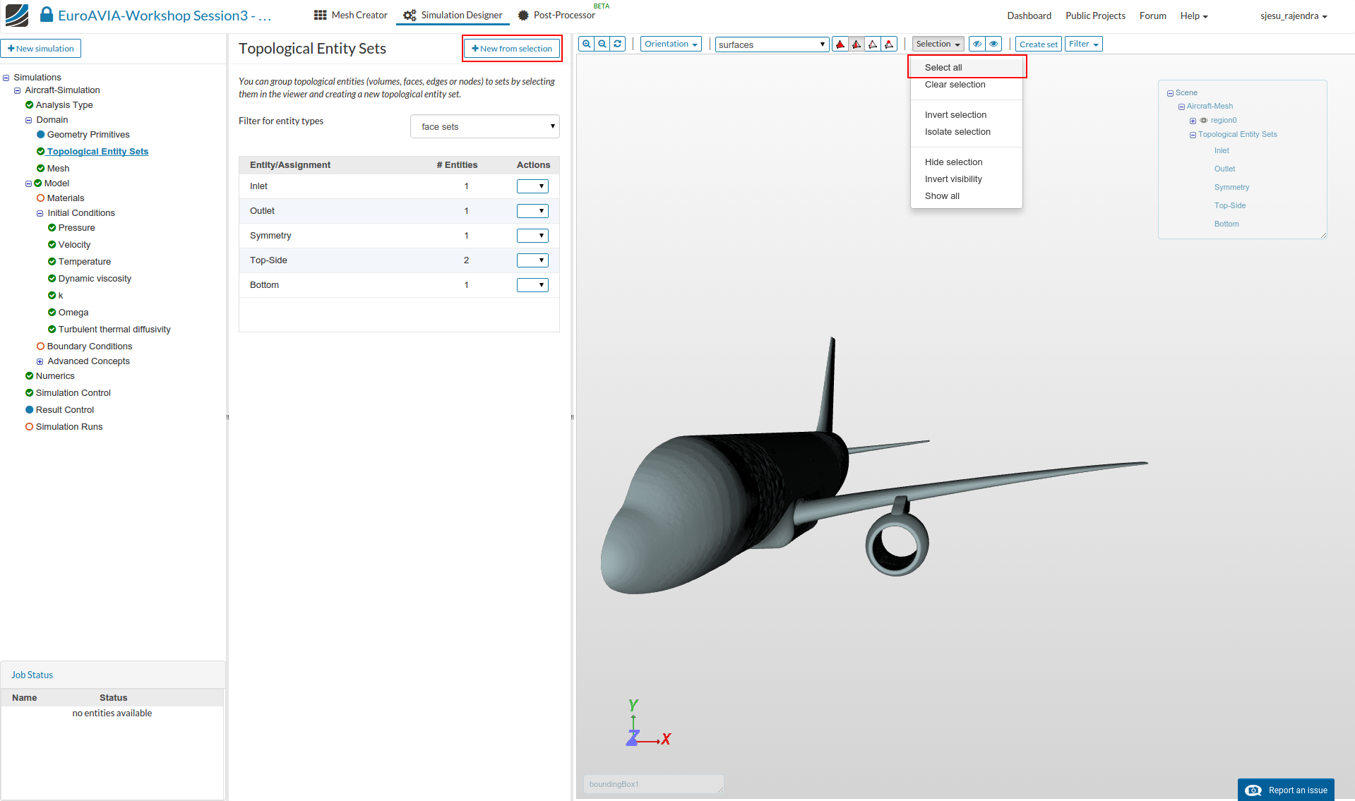
- Click Select all form the selection list and name it as ‘Aircraft’.
Select Fluid Material
- Select ‘Material’ from the sub-tree and click New.
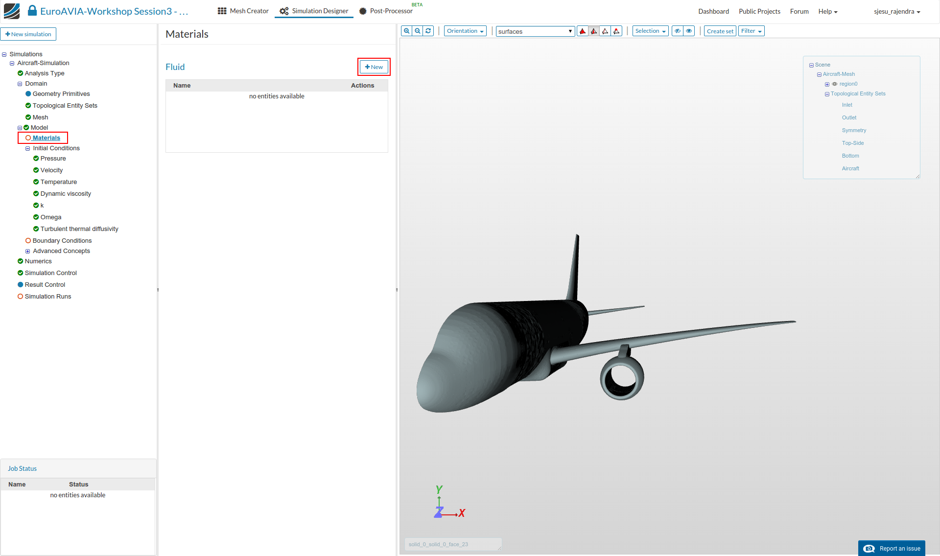
- Select Import from material library in the top of the pane.

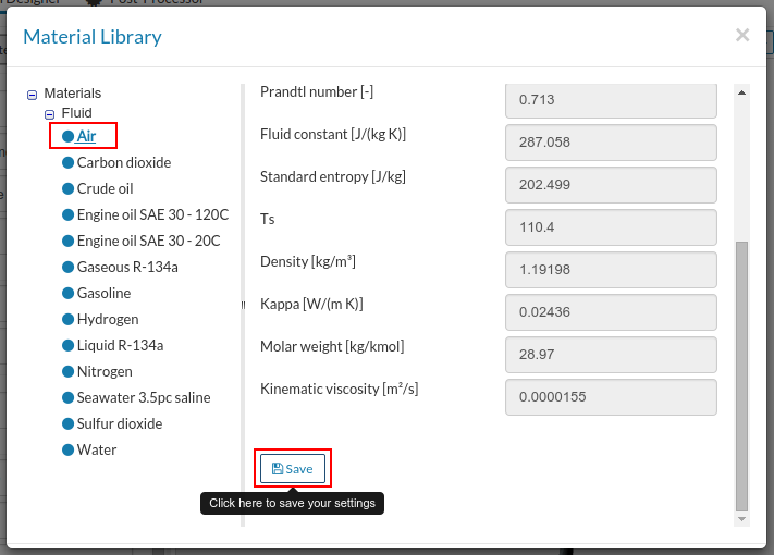
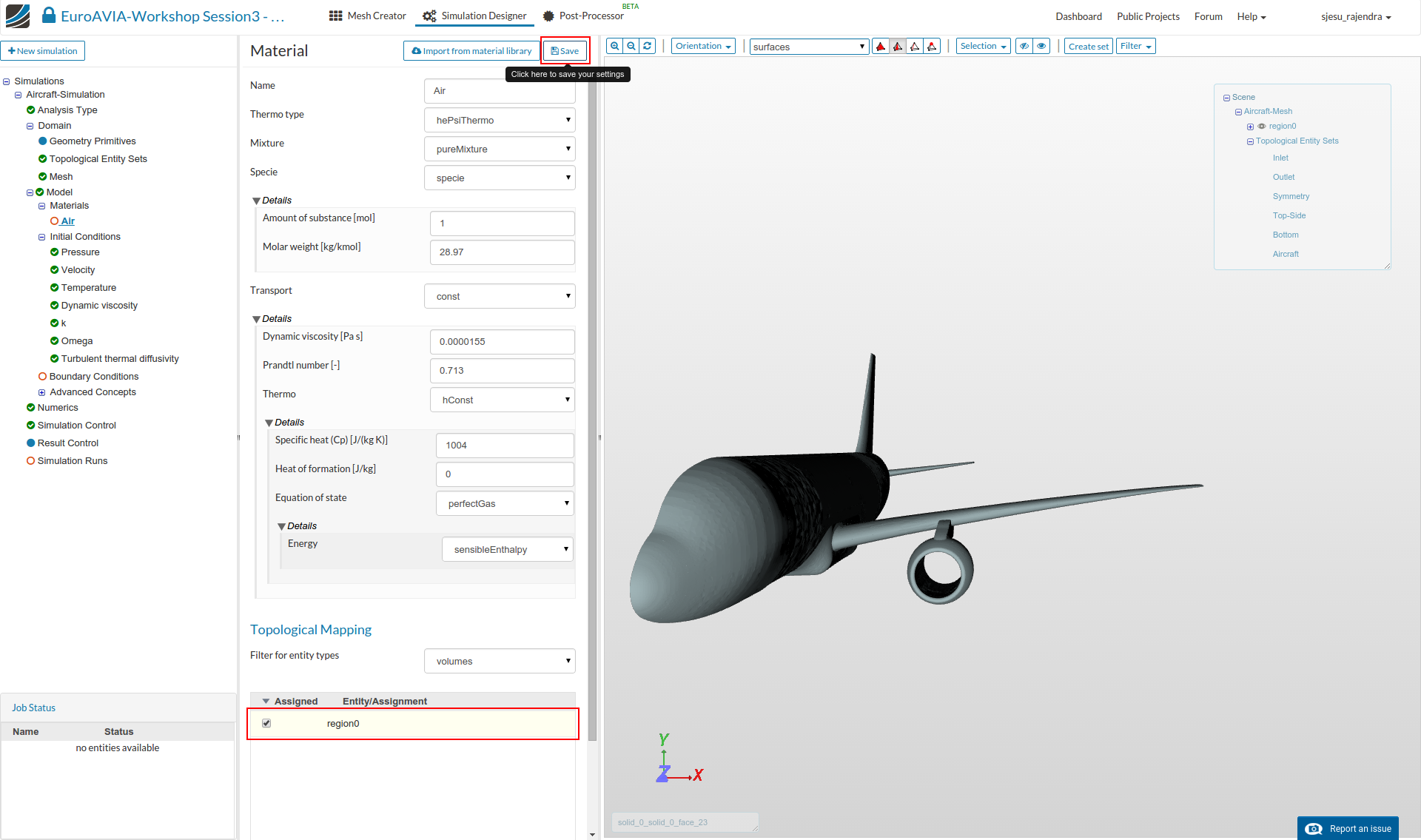
- Click Air and select the Save button.
- Select region0 from Topological Mapping and click the Save button.
Initial Conditions
- Default initial conditions can be maintained for the simulation runs.
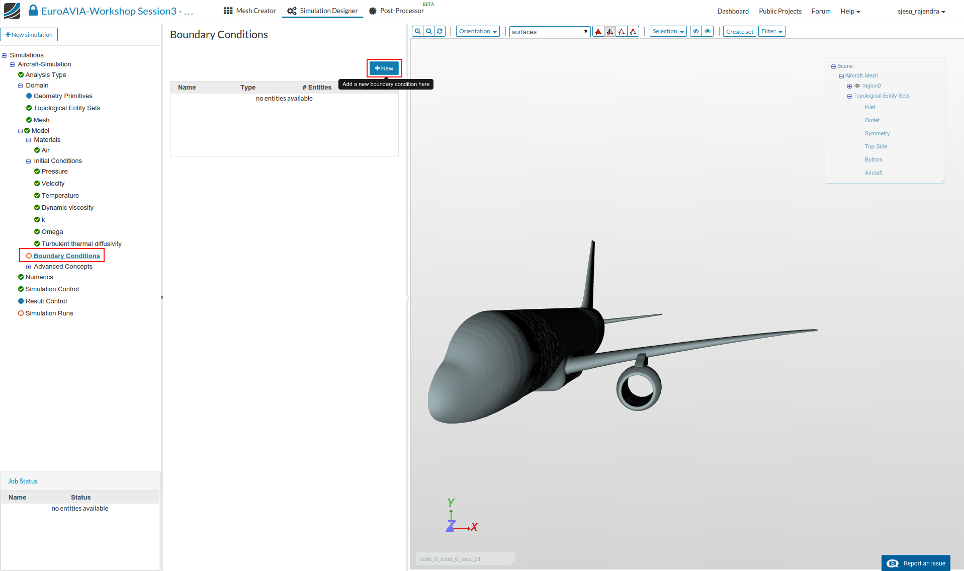
Boundary Conditions
The boundary conditions define the flow variables at the boundary surfaces.
- Click on ‘Boundary condition’ and select New.
Inlet :
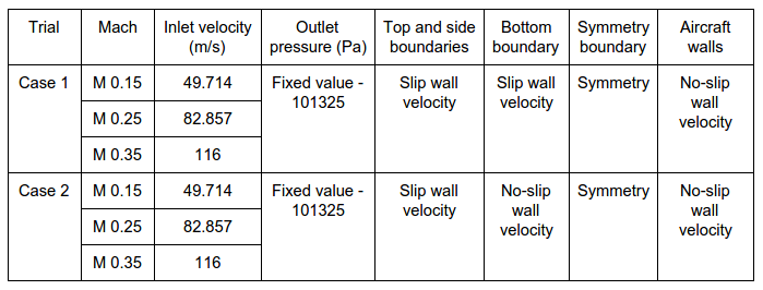
- Enter the inlet boundary condition with a z-direction velocity of -49.714 m/s and temperature value as 273 K. * Select the Inlet entity and click Save option.

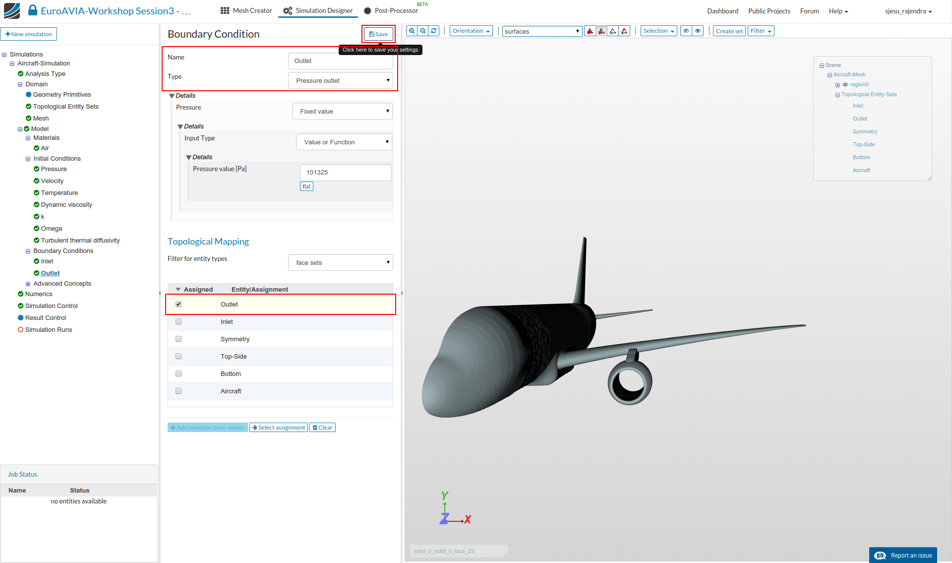
Outlet :
As the velocity is not known at the outlet faces, we would define the pressure here.
- Select a pressure outlet boundary condition, select the outlet entity and click Save option.
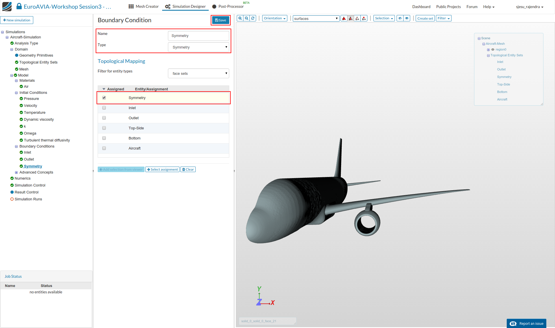
Symmetry :
- Next we will create the symmetry condition.
- Select a Symmetry boundary condition, select the symmetry entity and click Save option.
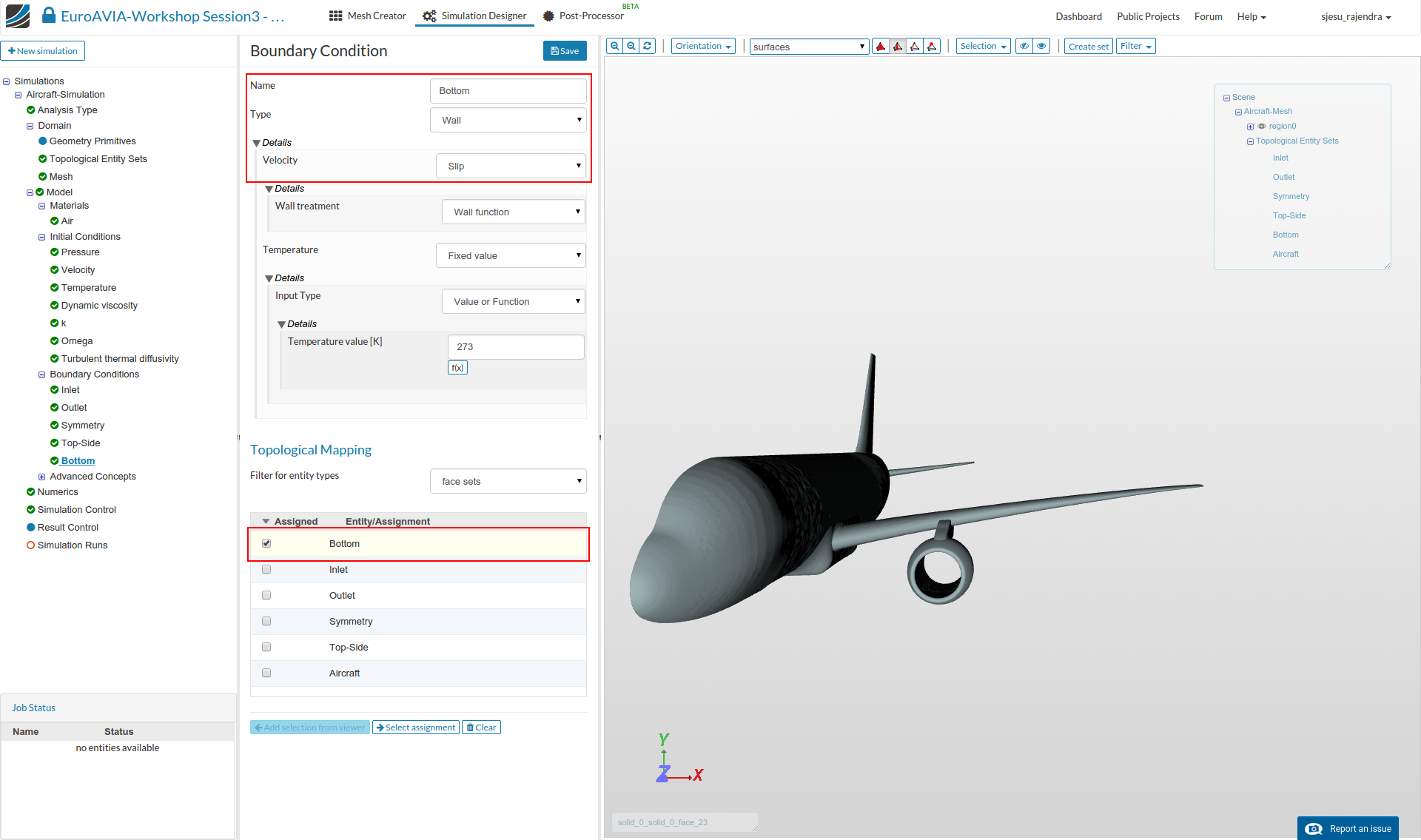
Top-Side and Bottom Walls :
- Create a boundary condition named Top-Side with Type Wall and velocity type Slip and temperature 273 K.
- Select the top, side entities and click Save option.

- Create a Bottom boundary condition similar to the previous, with Type Wall and velocity type Slip and temperature 273 K.
- Select the bottom named entity and click Save option.

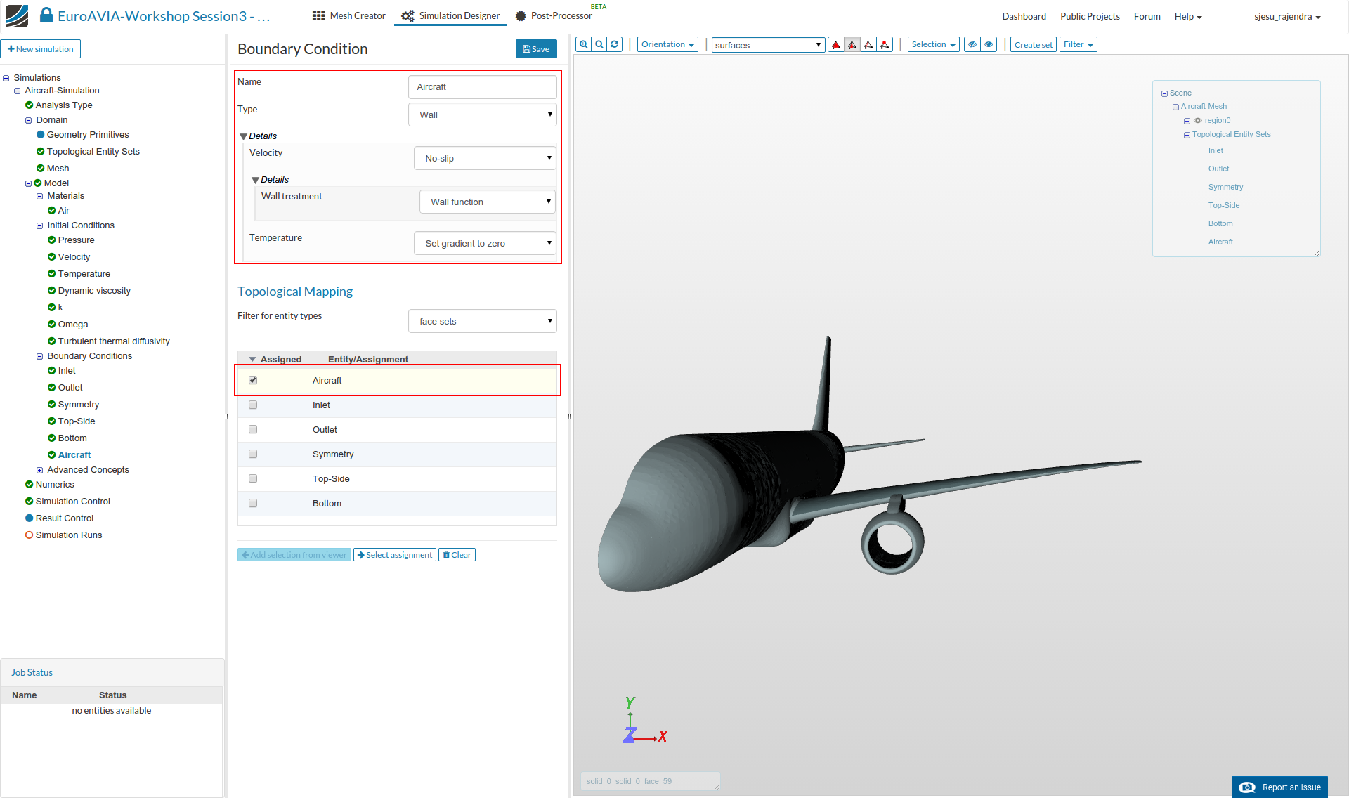
Aircraft - Walls :
- The remaining boundary definition is for the Aircraft - Walls.
- create a New boundary condition of type “Wall” and velocity type with No-slip and Zero gradient temperature condition.
- Select the Aircraft entity and click Save .
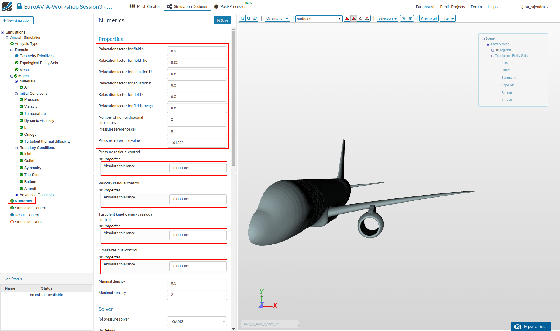
Numerics
-
Select ‘Numerics’ from the sub-tree and enter the following values. This enhances the solver to get the appropriate results.
-
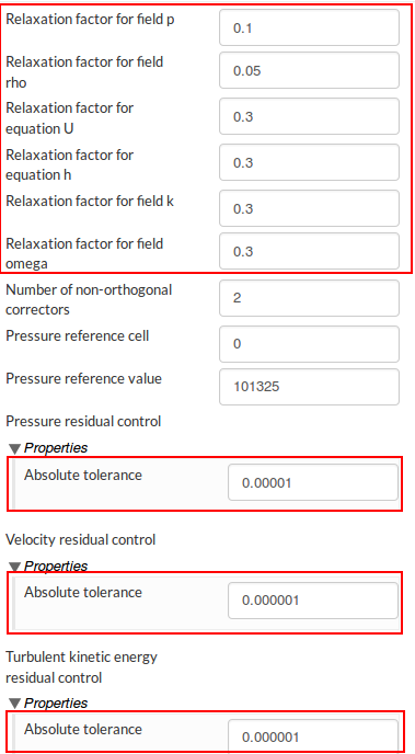
Set the relaxation factors to:
p : 0.2
rho : 0.05
U : 0.5
k : 0.5
Omega : 0.5
Number of non-orthogonal correctors : 2
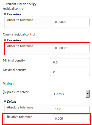
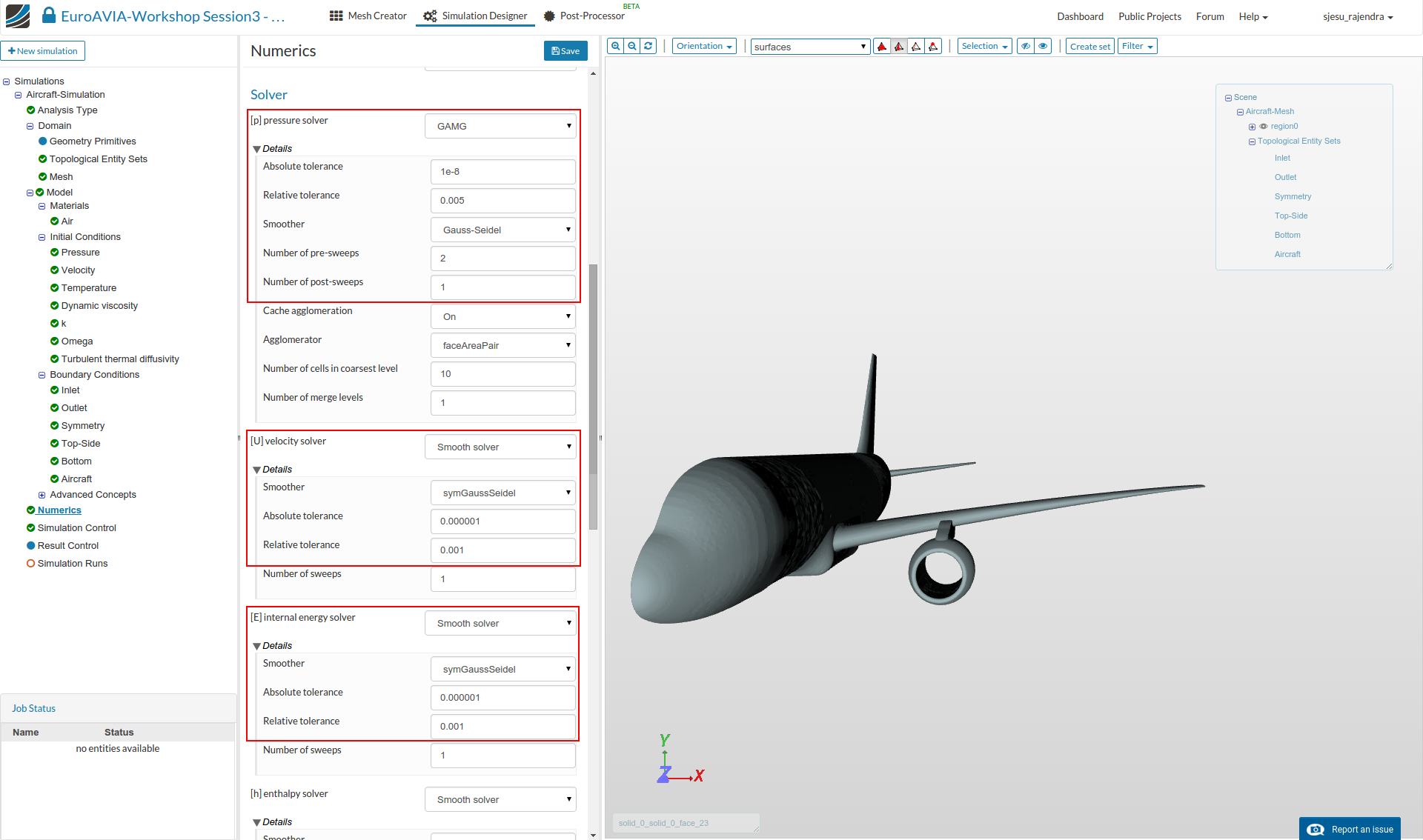
- The absolute tolerances for all residuals are changed to 0.000001
-
Change the pressure solver to GAMG with absolute and relative tolerances to 1e-8 and 0.005 respectively. The pre- and post-sweep have to be changed to 2 and 1 respectively.
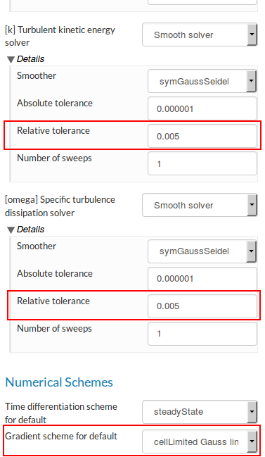
-
All other solvers should be changed to Smooth solver type with absolute tolerance 0.000001 and relative tolerance 0.001.
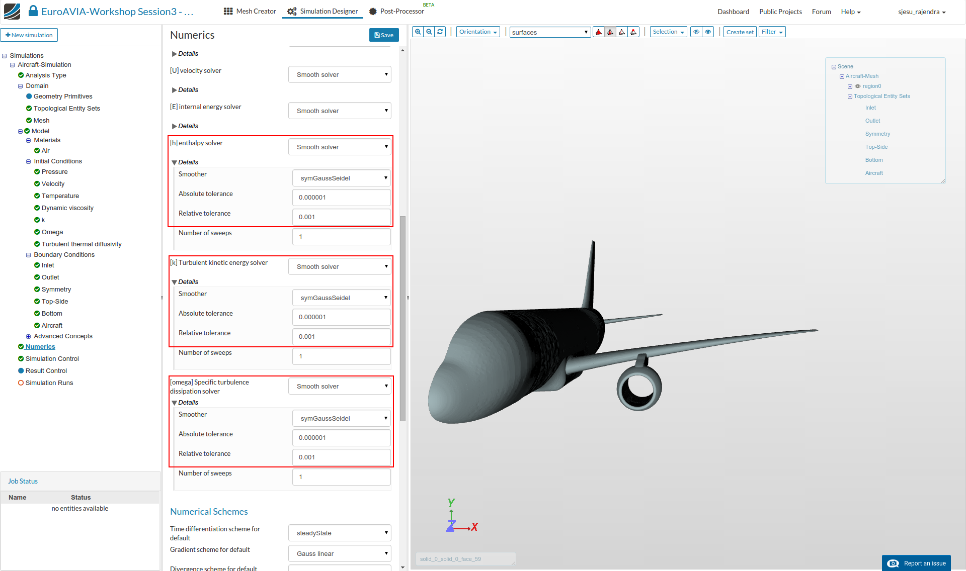
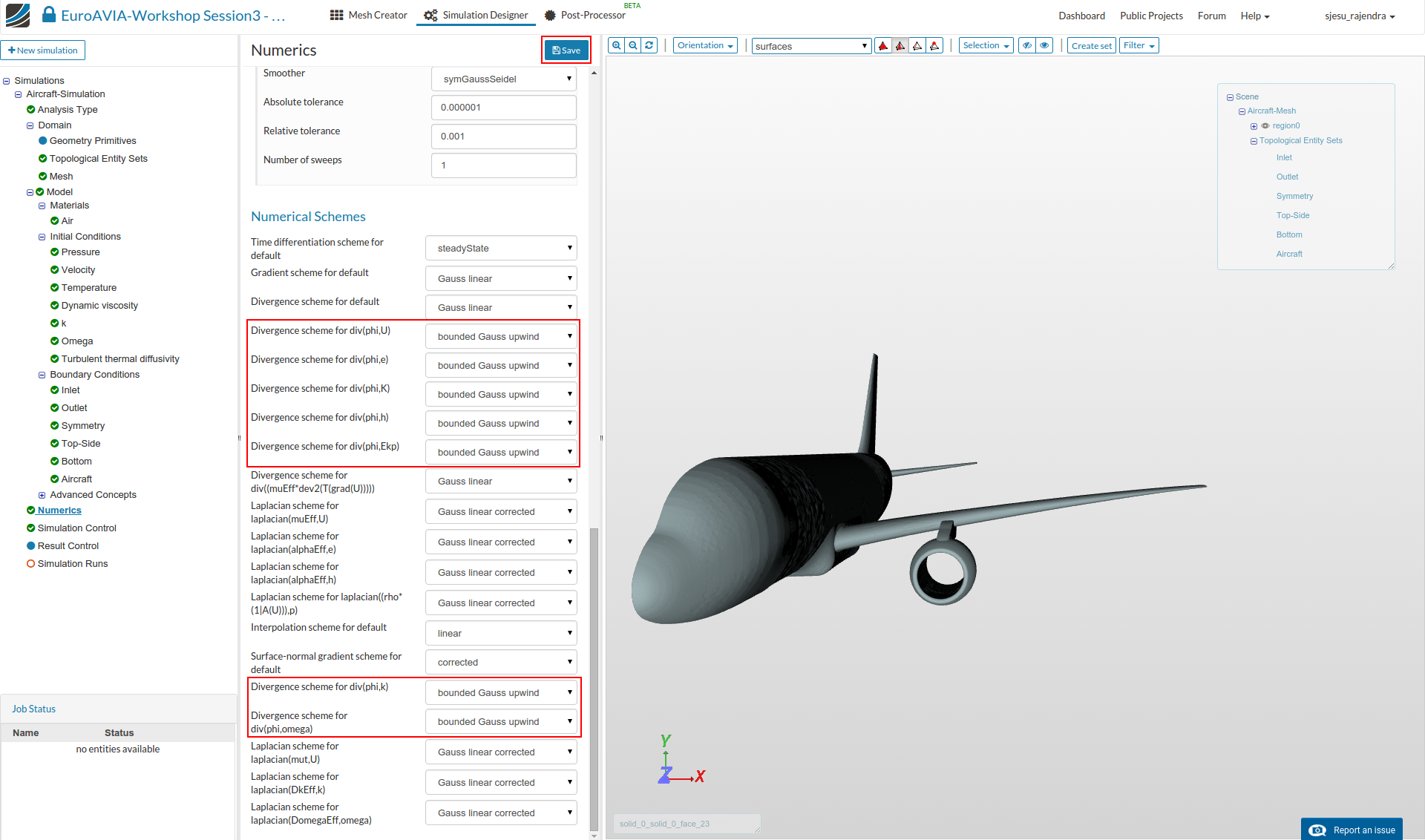
- Set the divergence schemes to bounded Gauss upwind.
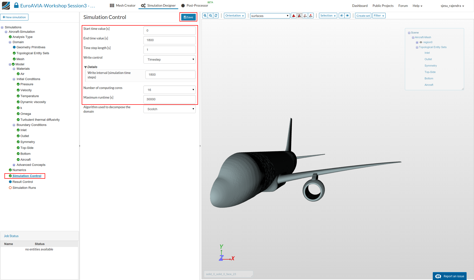
Simulation Control
- Click on ‘Simulation control’ and setup the simulation run for 1800s time with a time step of 1.
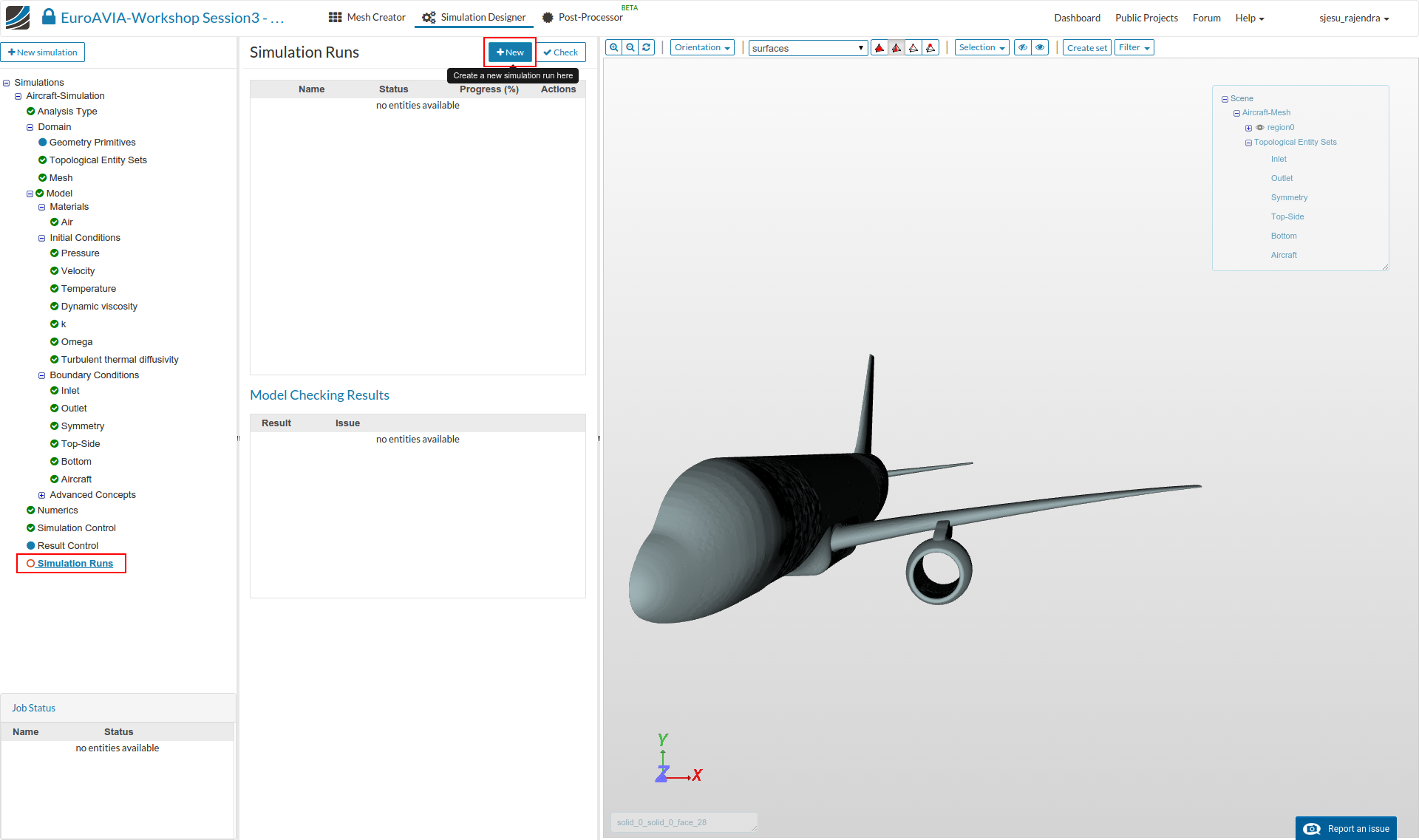
Create New Run
- Click on Simulation runs and create a new run.
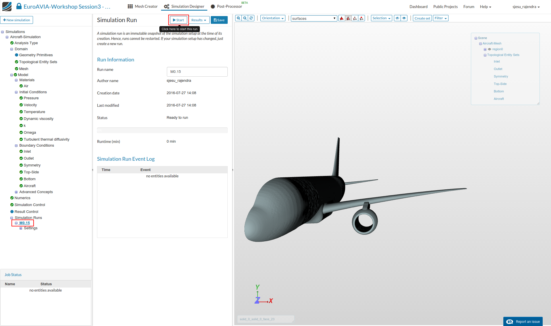
.
- Create new simulations for Mach 0.25 and 0.35 by duplicating this simulation. Enter the new velocities as follows.
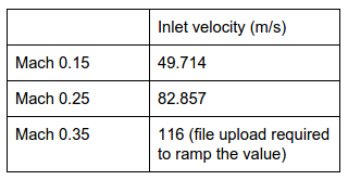
- The following file has to be uploaded to define ramping of inlet velocity .
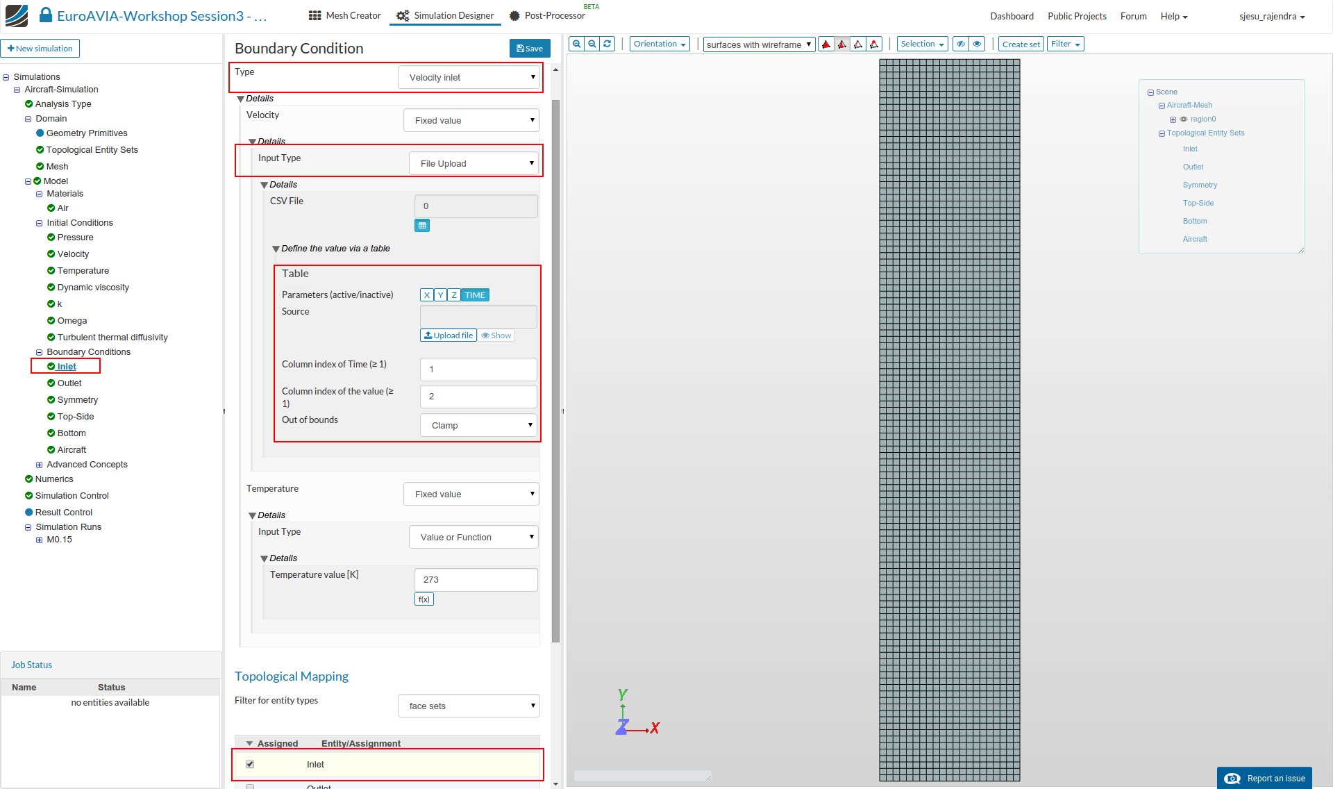
Modify Inlet boundary condition for M=0.35
- For Mach 0.35 the file upload for ramping the inlet velocity is done as shown in the image below. Make sure to have the following properties for file upload.
- Select Velocity Input Type : File Upload
- Unselect X button under paramaters and select TIME button so that we ramp the velocity over time.
- Change ‘Column index of Time’ to 1 and ‘Column index of value’ to 2.
- Select the Inlet entity and click Save.
- The simulation takes between 160 to 200 mins to finish.
For the next set of simulations with aircraft close to ground, duplicate one of the simulation and follow these steps.
-
Click Domain from the tree and select the new mesh created with the aircraft close to ground.
-
Go to Topological entity sets and create similar sets for inlet, outlet, symmetry, top-side, bottom and aircraft walls for the new mesh.
-
Assign the material air to the new region.
-
Assign the boundary conditions to the new topological entities created.
-
Duplicate the simulation for new cases Mach 0.25 and Mach 0.35 with inlet velocities shown in the table above.
Post-processing
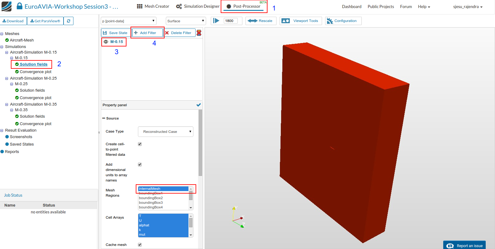
- Once the simulation is over switch to obtain the results by clicking on Post-processor tab on the top. Select the solution field (M-0.15 in this case). Note that the solution field by default includes the internal mesh.
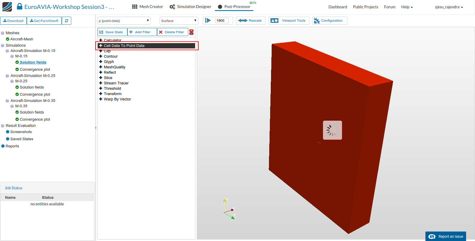
- Click on Add filter and select Cell Data to Point Data. This is used to obtain the point data solutions to all the sub-filters of this solution field.
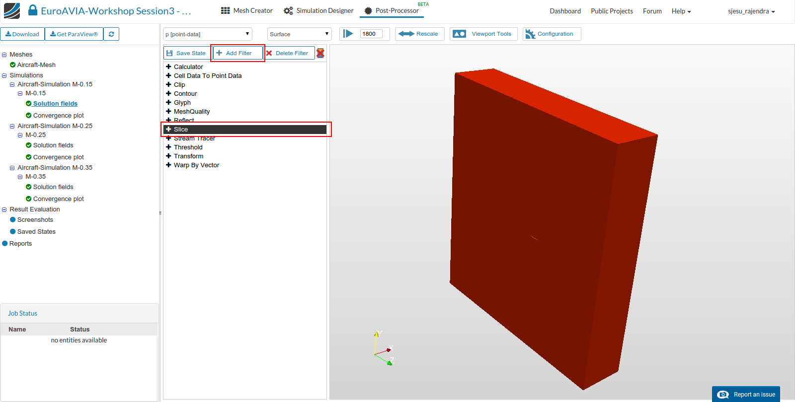
Slice Filter (2D):
- Select the new filter created ‘CellDatatoPointData1’ and click Add filter option to select Slice. We include a slice to the domain in order to see the wake behind the aircraft and also the density variation of the flow.
- Apply the following slice properties and click the ‘Tick’ icon to apply.
Slice type - Plane
Origin - default values (0.0011, 0, 0)
Normal - (1, 0, 0)
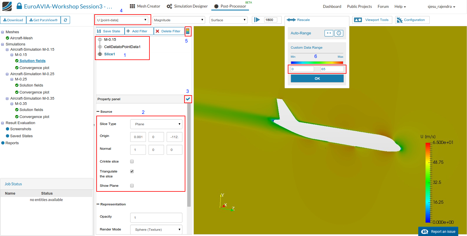
-
Select the velocity data U [point data]. Click on the ‘Color bar’ below the selection panel to view the ‘legend’ bar and re-scale it between 0 to 65 m/s.
-
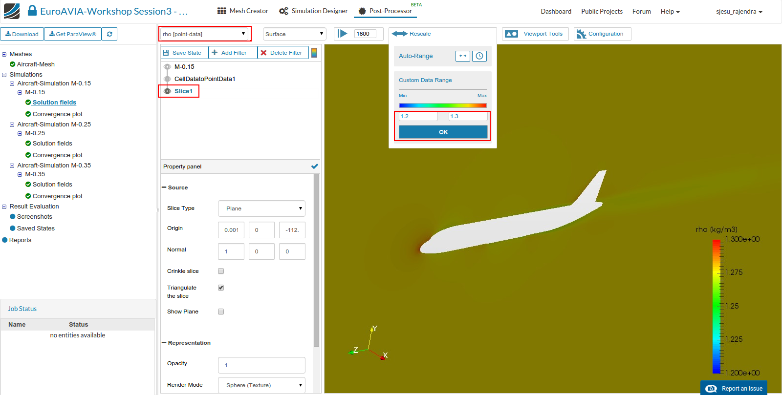
To show the density, select the slice and set data to rho [point-data]. Select the data range between 1.2 to 1.3 kg/cu.m.
Surface contours:
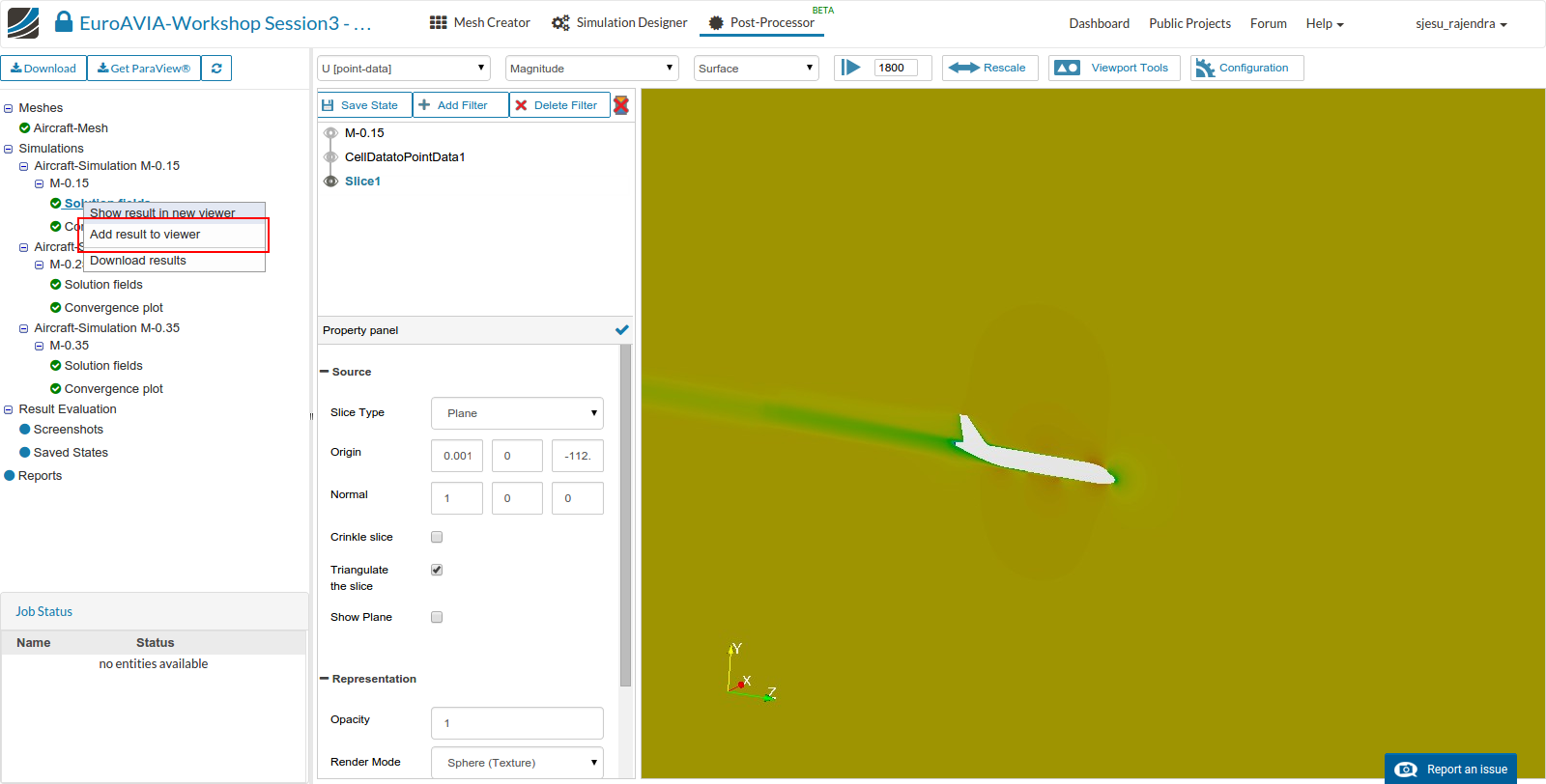
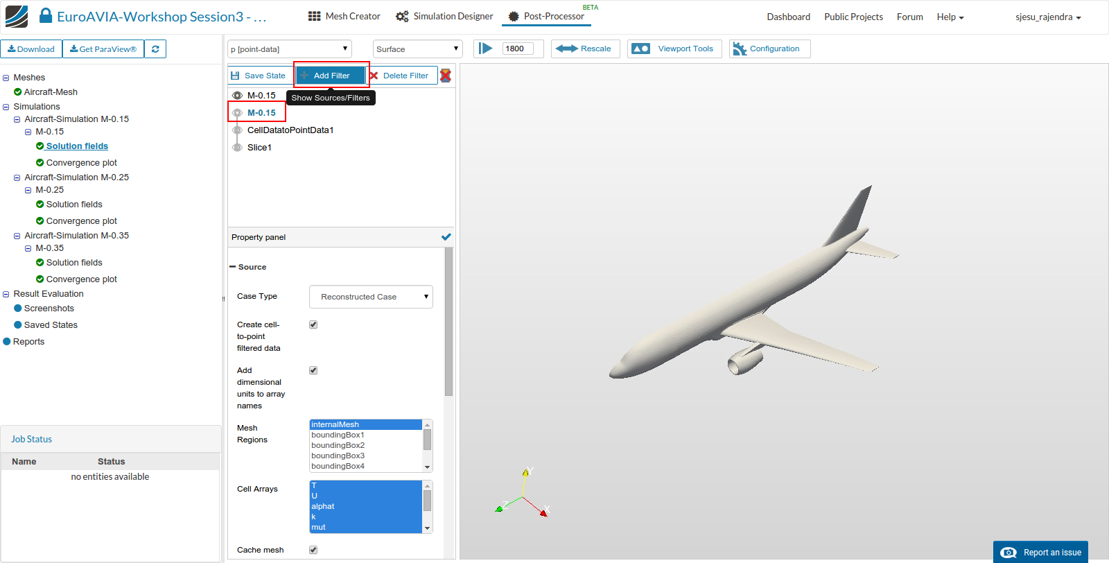
- Surface contours are added to get the pressure distribution on the aircraft surface. In order to do this, right click on the solution field and select Add result to viewer. This by default introduces the internal mesh.
- Go to Mesh Regions from the property panel and select all the surface walls of the aircraft, i.e. from solid_0_solid_0_face_0, solid_0_solid_0_face_1,… until solid_0_solid_0_face_61. This can be done by clicking the first face solid_0_solid_0_face_0 and then scroll down and ‘Shift+last face(solid_0_solid_0_face_61)’. Select the Tick to apply.
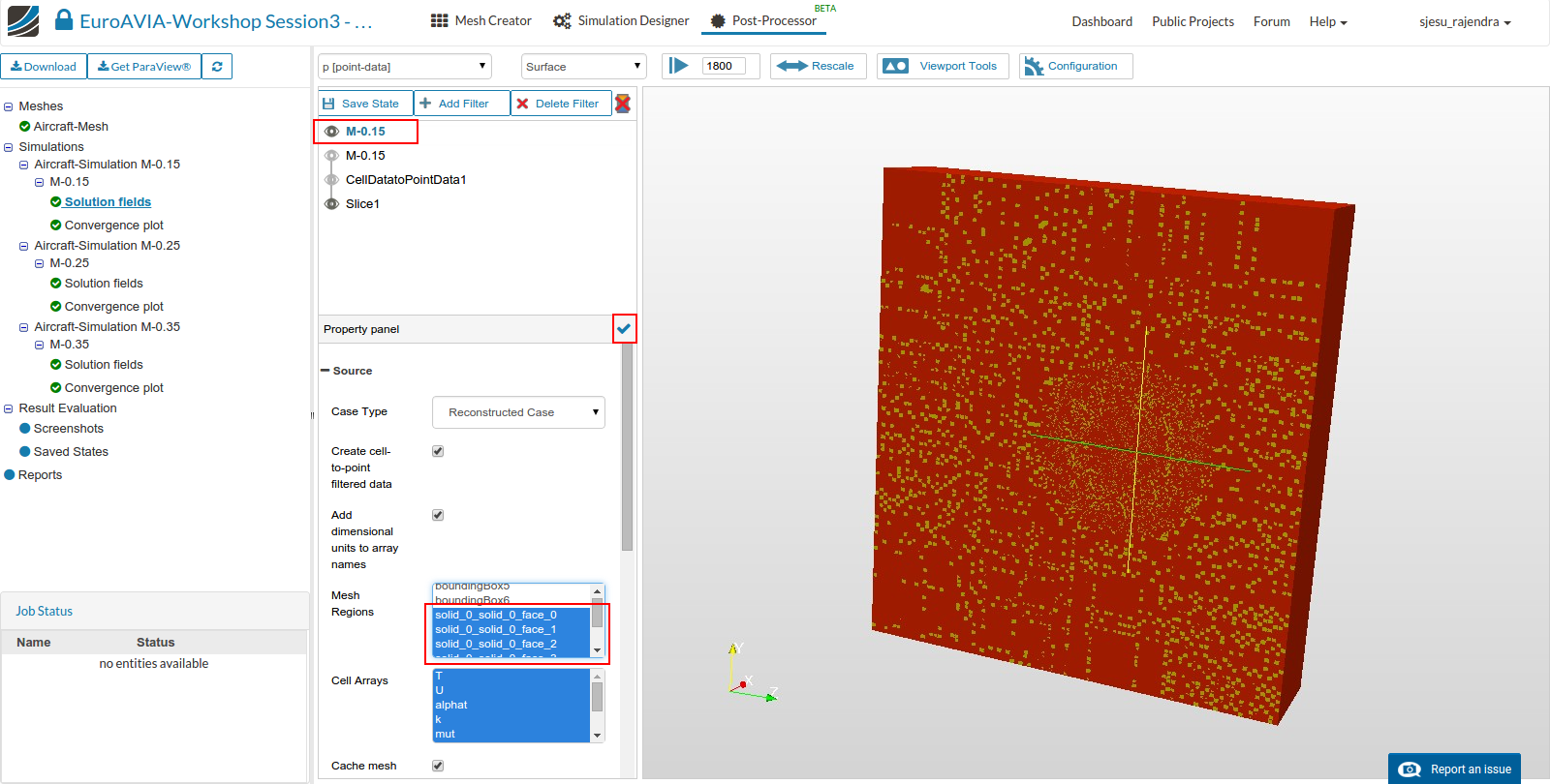
- Select the data to be p [point-data] and select the data range to be 90000 Pa to maximum value in the domain.

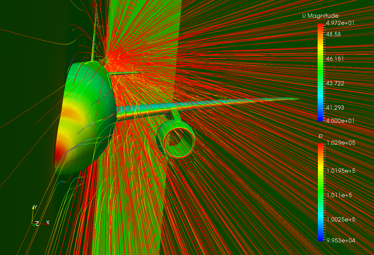
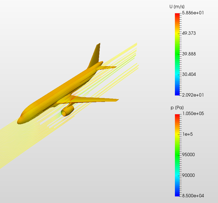
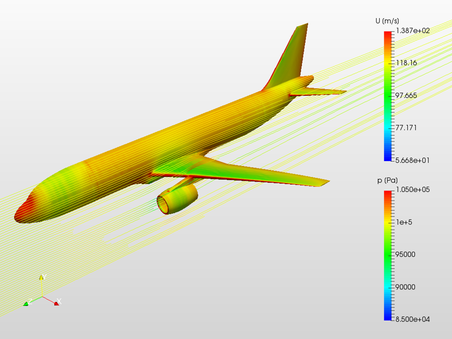
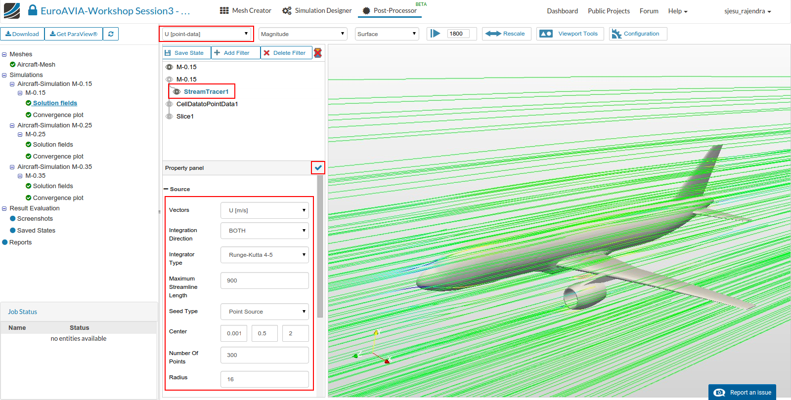
Streamlines:
- Hide the slice by clicking the small round next to the slice. Select the internal mesh solution field and click Add filter, for inserting Stream tracer in order to get the flow streamlines. Change the display field to U [point data] and enter the following values to create a point source stream tracer (Please leave the other properties with default values).
Vectors - U
Maximum Streamline Length - 900
Seed Type - Point Source
Center - (0.0011, 0.5, 2)
Number of points - 300
Radius - 16
- and click the ‘Tick’ icon to apply.
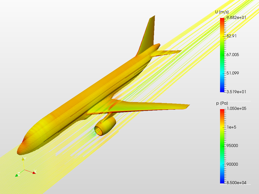
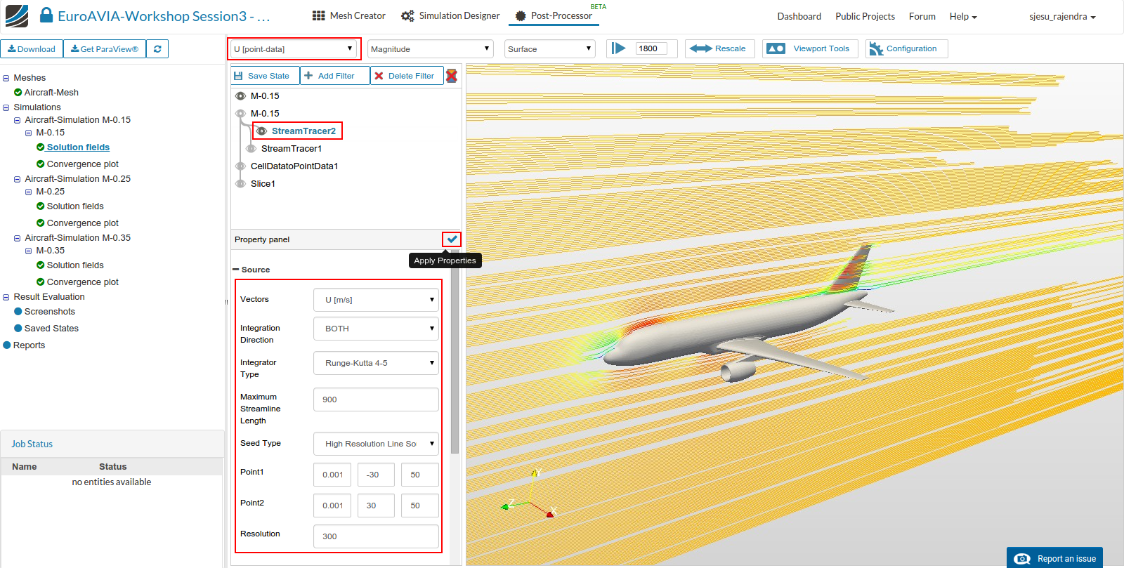
- Another streamline with line source can also be added to visualize yet another interesting flow in the domain.
Vectors - U
Maximum Streamline Length - 900
Seed Type - High Resolution Line Source
Point1 - (0.0011, -30, 50)
Point2 - (0.0011, 30, 50)
Resolution - 300
Updated:
-
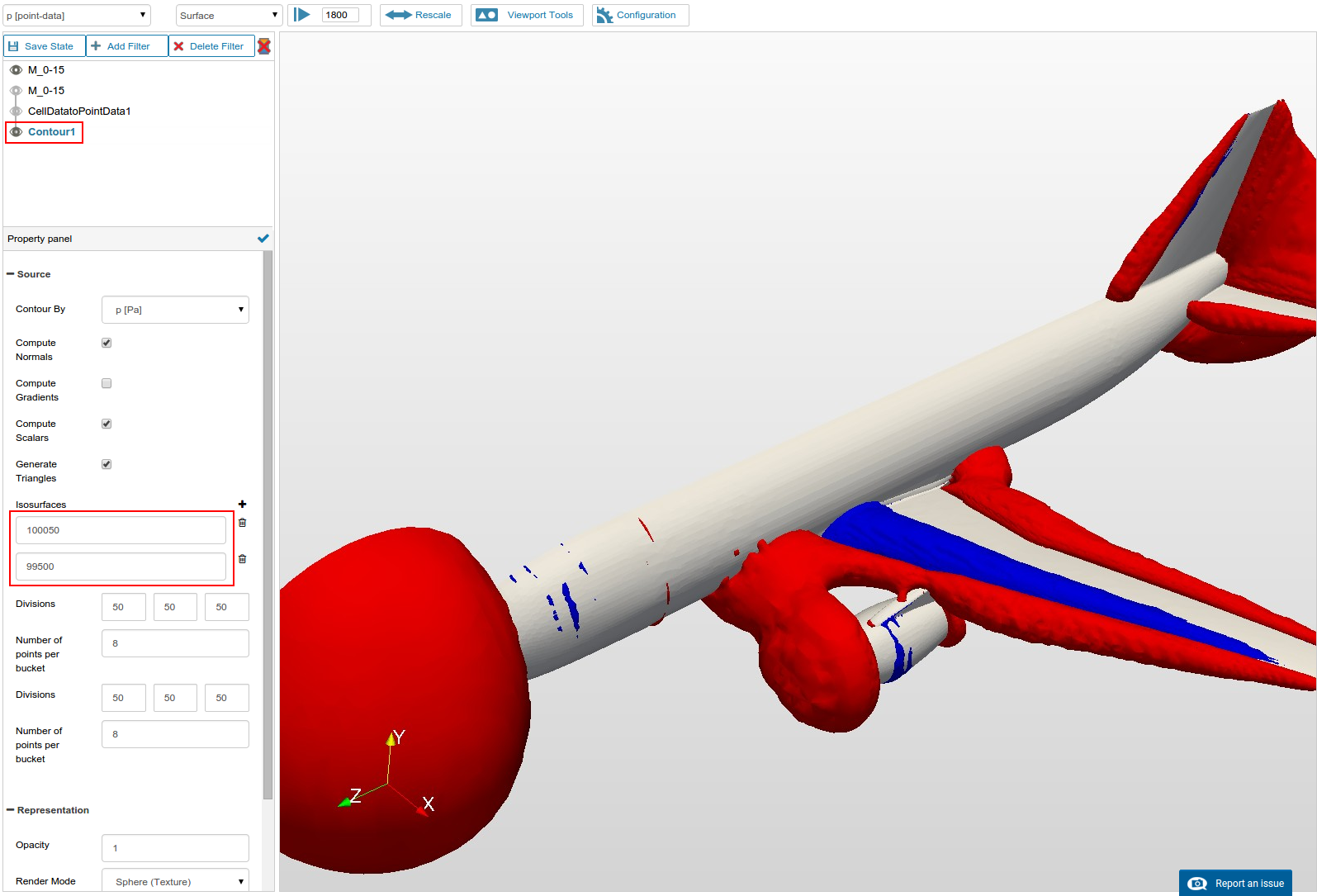
A contour plot can be obtained from the point data by adding isosurfaces at 2 different pressure values as shown.
Isosurface 1 - 100050
Isosurface 1 - 99500 -
Furthermore density contour can also be plotted by mentioning the ‘rho’ values between a specific range.
- Similarly perform the post-processing of the configurations and compare!