This post is a continuation of Aerospace Workshop Session 3 - Part I. It contains the tutorial to setup the simulation for Aerodynamics of an aircraft.
Simulation Setup
A total of 3 different inlet velocities will be simulated. For the sake of simplicity, this step-by-step simulation setup will focus on 0.15 Mach and can be easily adapted to other velocities.
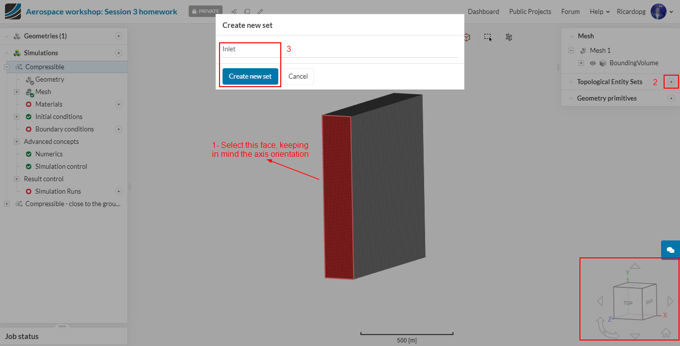
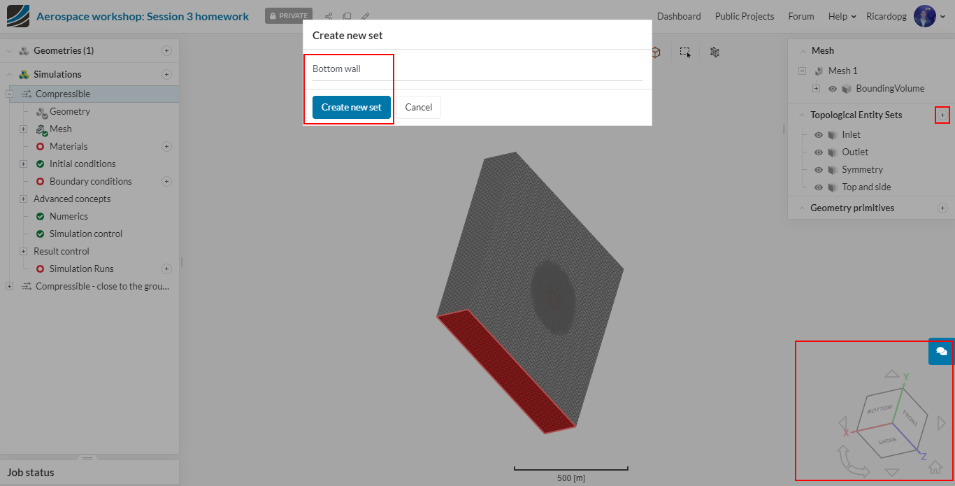
Let’s create Topological Entity Sets to help us setting up Boundary Conditions later on. A new topological entity set is assigned as follows:
- Left click on all faces that will constitute a topological entity set;
- On the right-hand side panel, next to Topological entity set, click on the + icon;
- Name your entity set as you deem suitable and click on Create new set.
Create an Inlet topological entity set as follows:
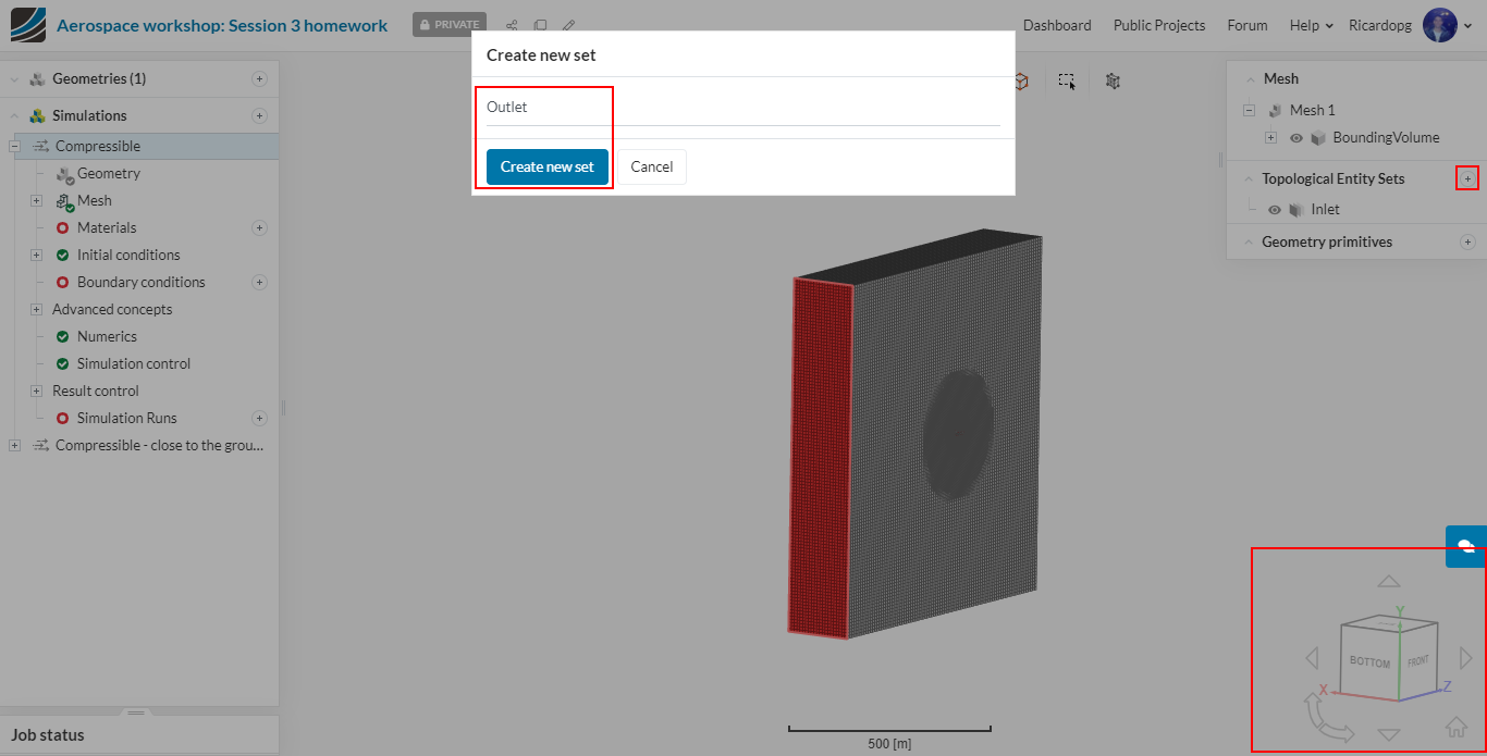
Similarly, create an Outlet topological entity set (the face is in the opposite side from the Inlet face):
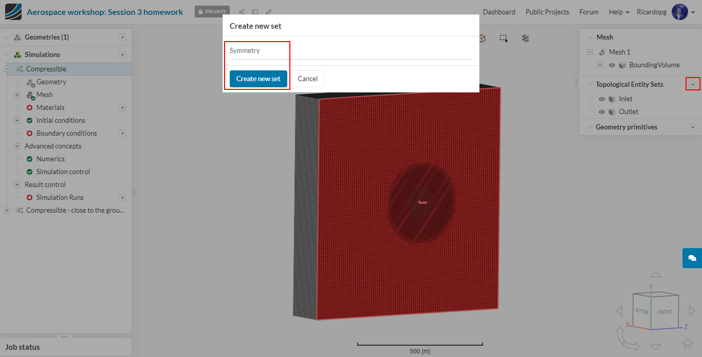
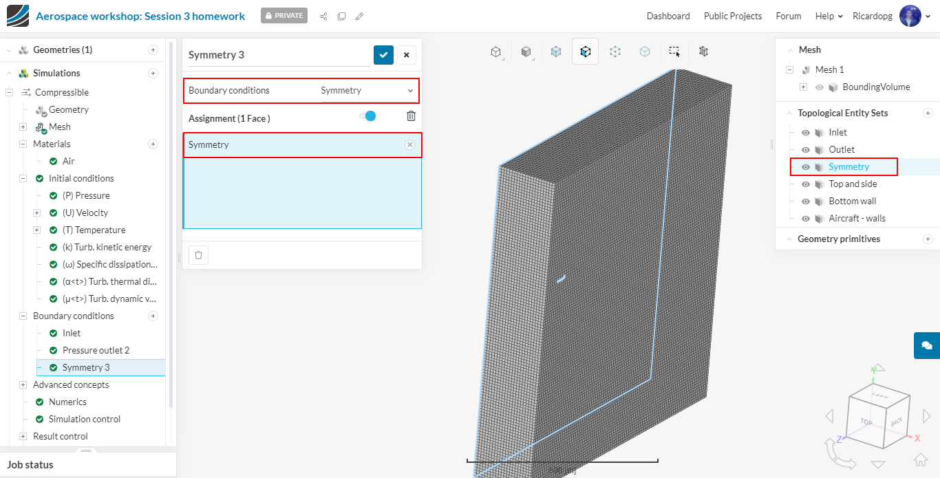
Create a Symmetry topological entity set as follows:
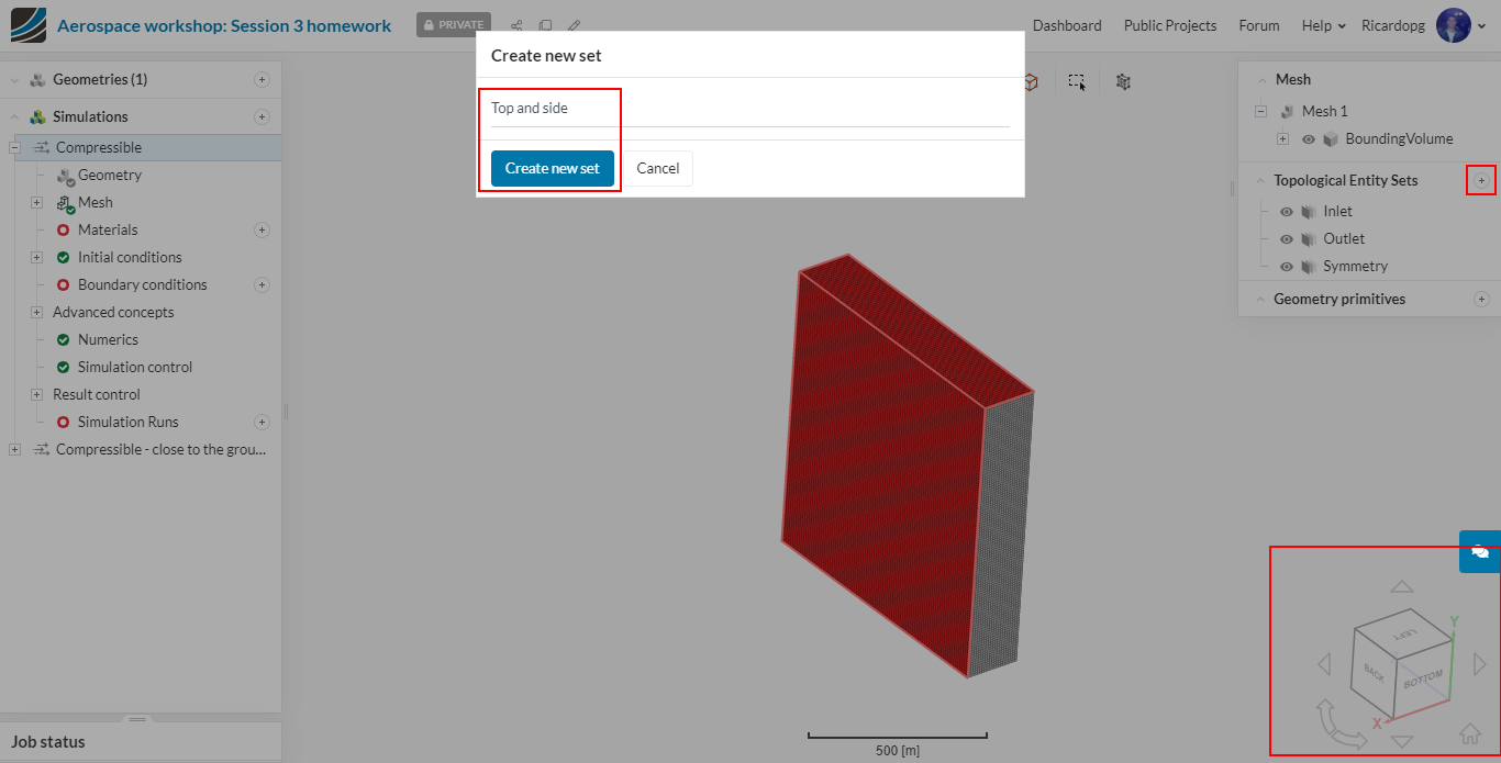
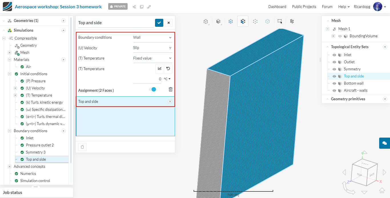
Create a Top and side topological entity set as follows:
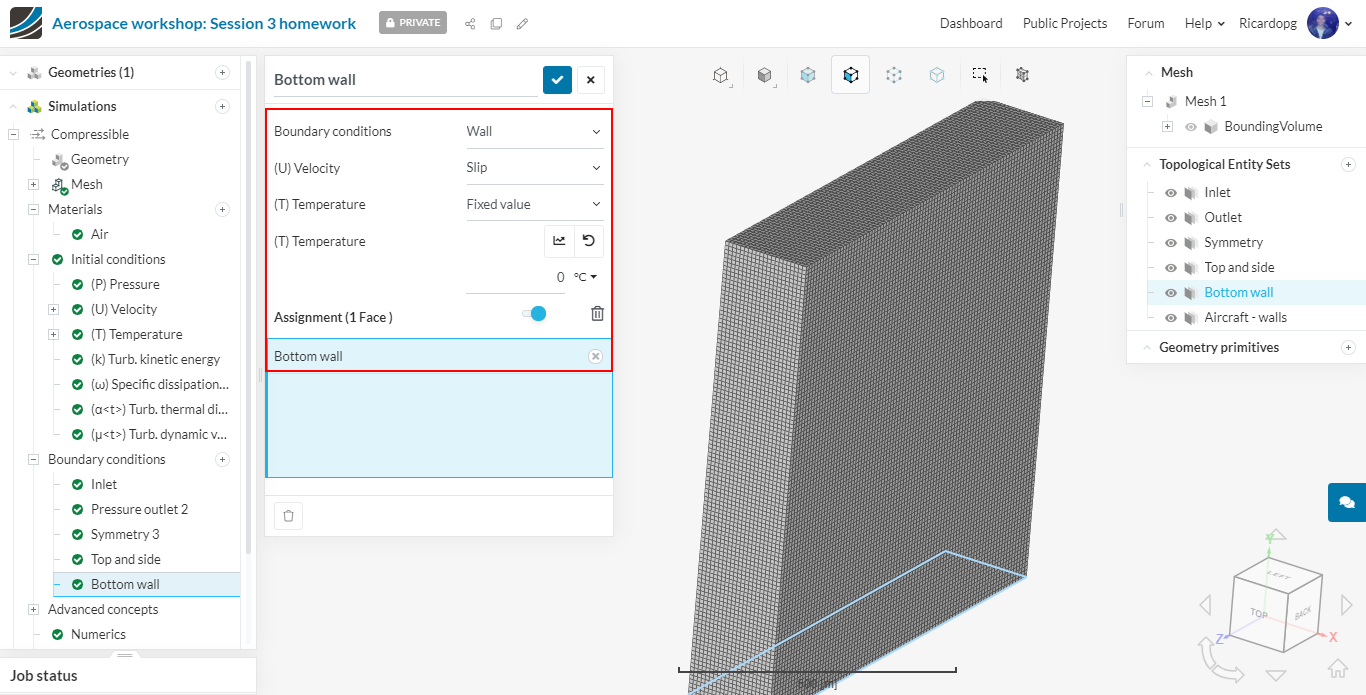
Create a Bottom wall topological entity set as follows:
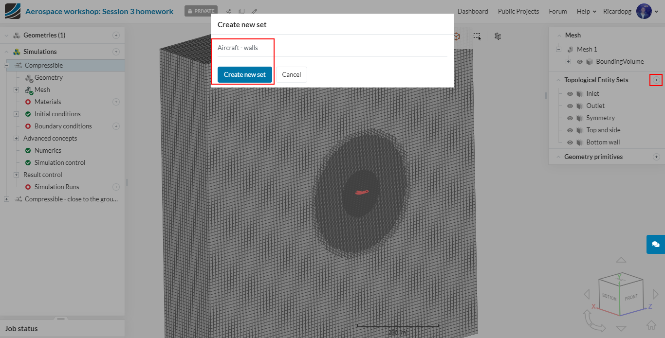
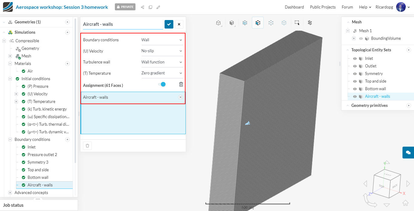
Create an Aircraft - walls topological entity set as follows:
There are ways to quickly select all surfaces from the aircraft. One of these ways is to first select all topological entity sets that have been previously created and then right click in the viewer to Invert selection:
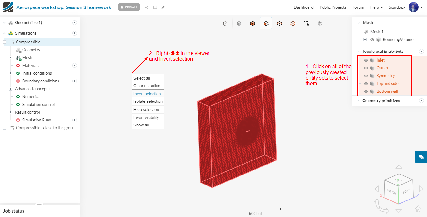
Conveniently, all the aircraft walls will be selected:
Select Fluid Material
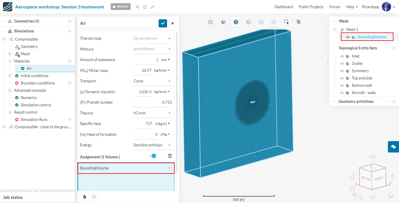
In the simulation tree, navigate to Materials. In the materials library, select Air and hit Apply:
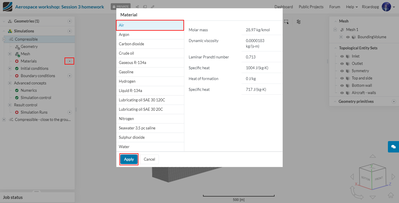
Air will be automatically assigned to the BoundingVolume. Just save and proceed to the next step.
Initial conditions
The parameters in each one of the cells are initialized by Initial conditions. Starting from there, the solvers will try to converge to a final solution. Having good estimates for initial conditions can, therefore, enhance the convergence rate.
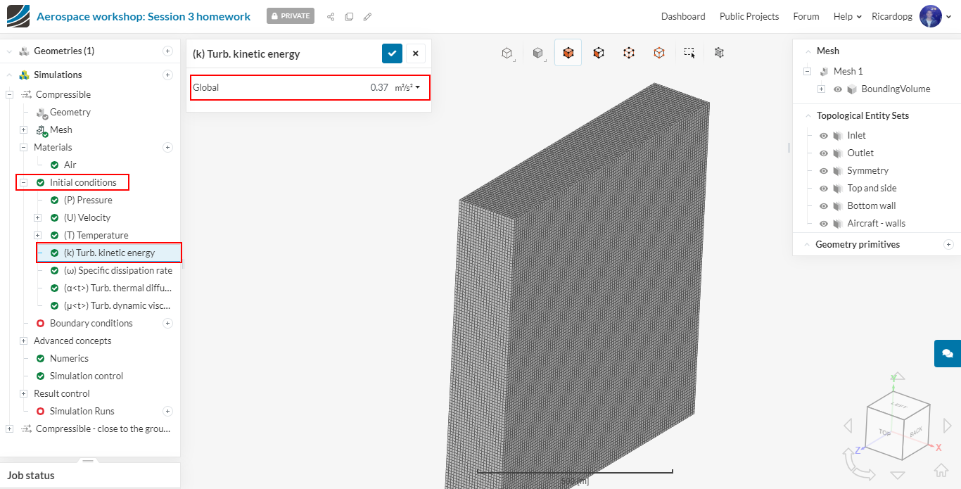
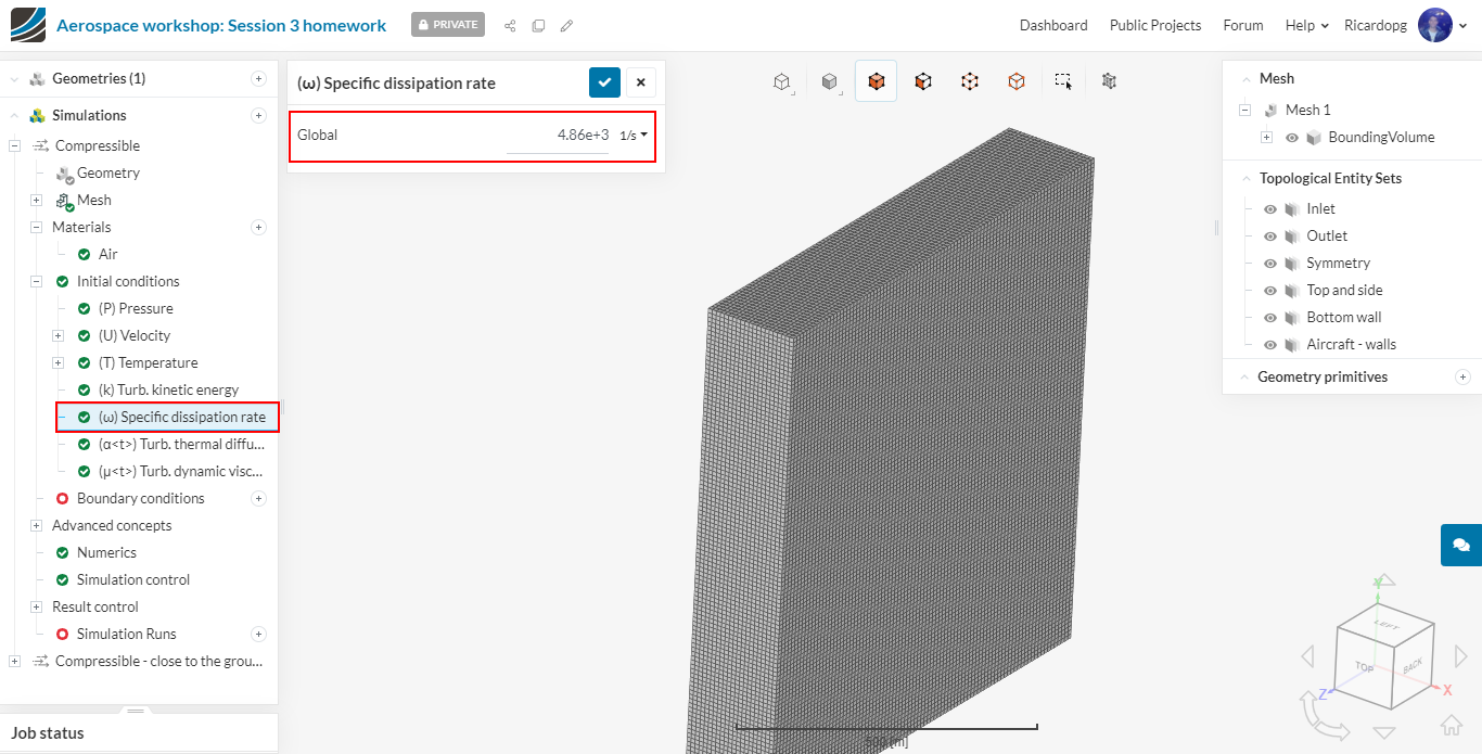
(k) Turb. kinetic energy and (ω) Specific dissipation rate can be estimated from these formulae. So, for external aerodynamics:
k=1.5*(I*U)^2
ω={ρk \over μ}*{1 \over {μt \over μ}}
In low turbulence flows, such as those in external aerodynamics of cars and airplanes, turbulence intensity (I) is in the order of 1%. In such cases, the parameter {μt \over μ}, known as Eddy Viscosity Ratio, can be considered to be in the range of 1 to 10.
The table below shows initial condition values for k and ω assuming turbulence intensity = 1% and eddy viscosity ratio = 5:
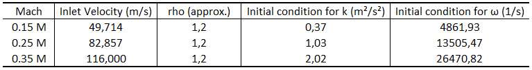
Please input these initial values in the corresponding fields:
Boundary conditions
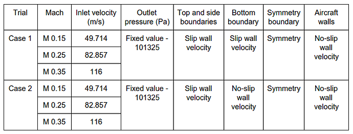
As a reminder from the first part of Session 3, here is the summary of the boundary conditions for the different setups:
The Boundary Conditions define the flow variables at the boundary surfaces. To add a boundary condition, click on the + icon and choose the appropriate type.
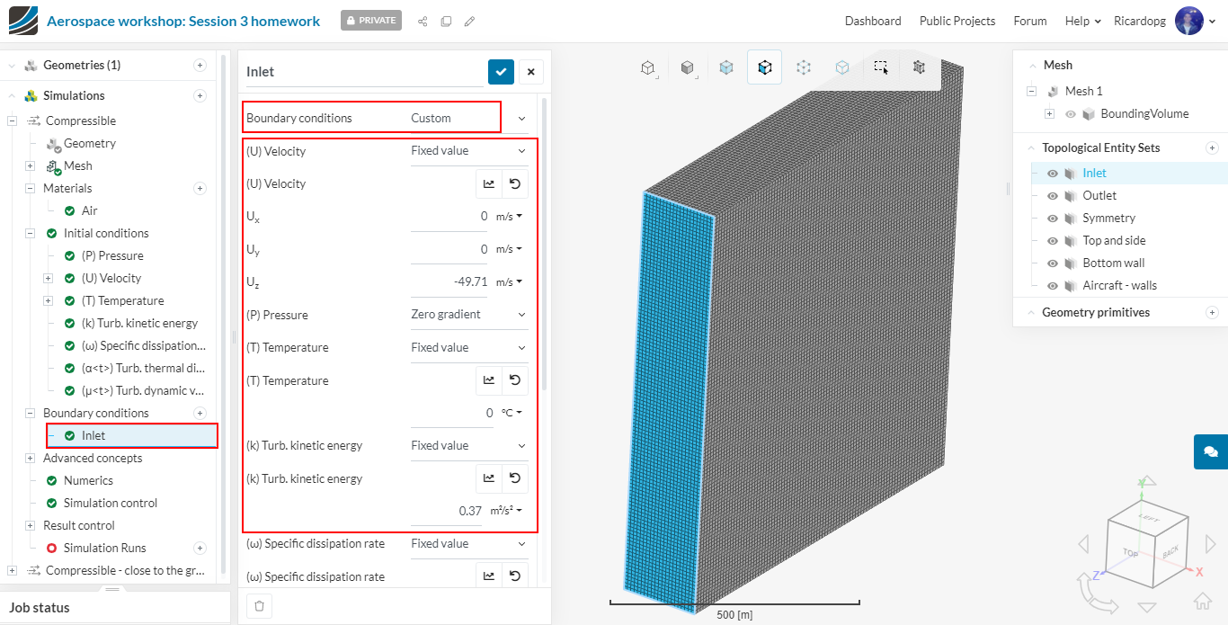
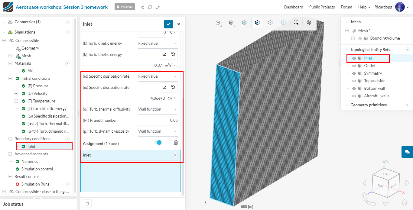
Boundary condition for the Inlet topological entity set: please create a Custom boundary condition and set it up as shown:
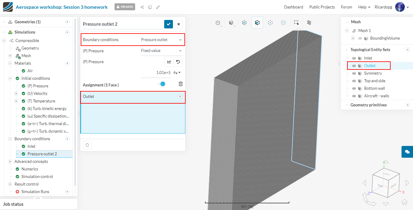
Boundary condition for the Outlet topological entity set:
Boundary condition for the Symmetry topological entity set:
Boundary condition for the Top and side topological entity set:
Boundary condition for the Bottom wall topological entity set:
Boundary condition for the Aircraft - walls topological entity set: it will be a Wall boundary condition with a No-slip condition for velocity and Zero gradient for Temperature:
Numerics
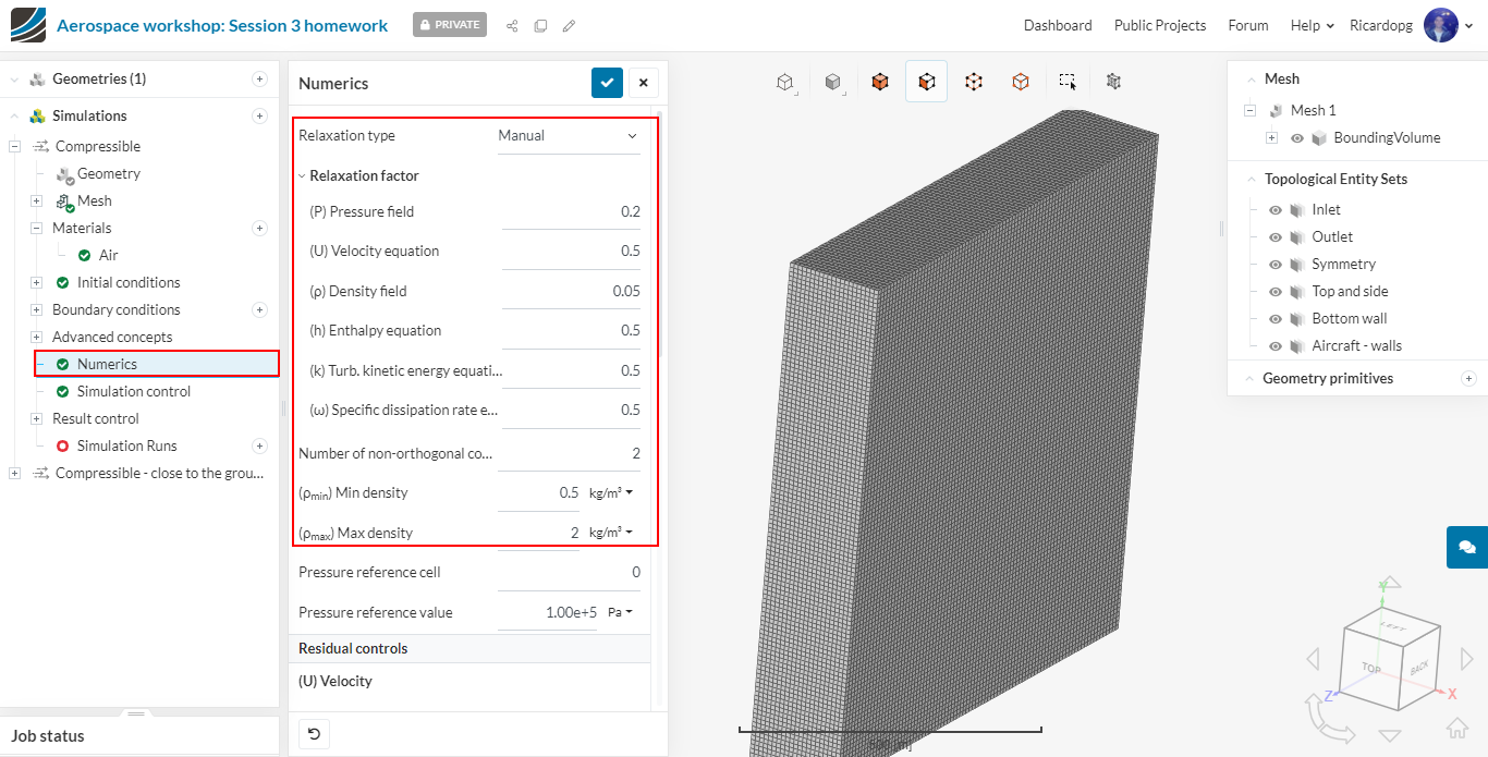
Select Numerics from the simulation tree and enter the following inputs. This enhances the solver to get the appropriate results.
- Set the relaxation factors to:
p: 0.2
U: 0.5
Density field: 0.05
Enthalpy equation (h): 0.5
k: 0.5
Omega: 0.5
Number of non-orthogonal correctors: 2
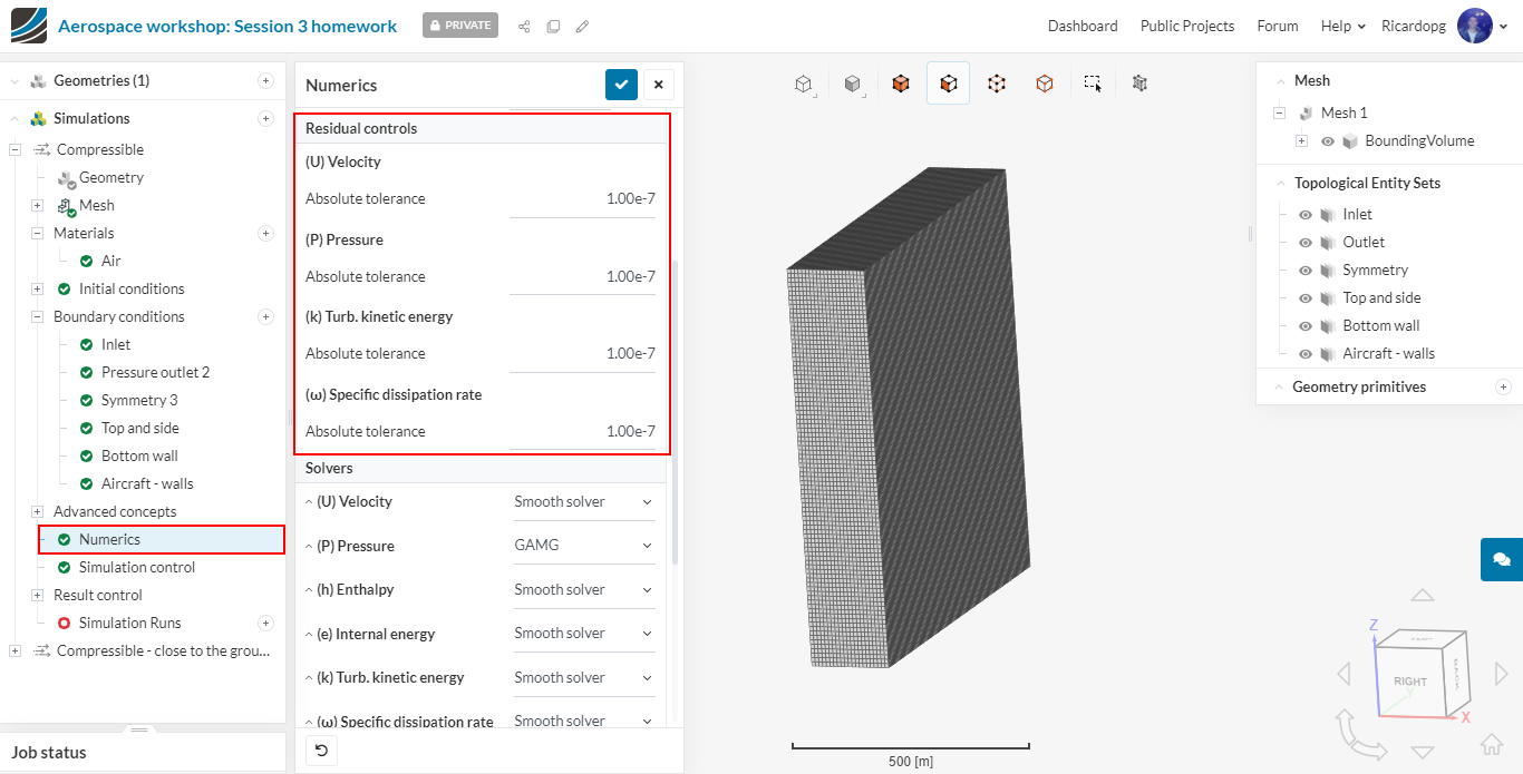
In Residuals control, set all values to 1e-7. When and if this criteria has been met, SimScale automatically stops the simulation. Otherwise it will run until the specified number of iterations has been achieved.
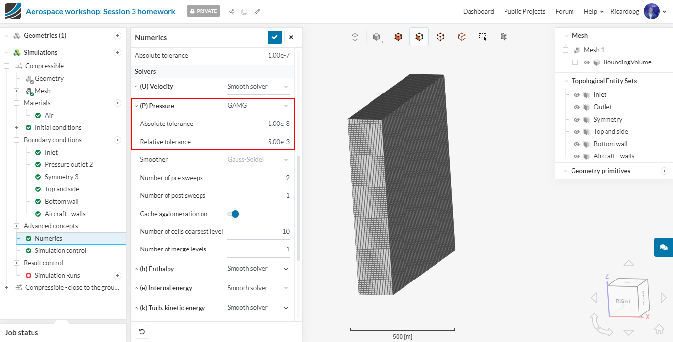
Change the pressure solver to GAMG with absolute and relative tolerances to 1e-8 and 0.005 respectively.
All other solvers should be changed to Smooth solver with absolute tolerance 0.0000001 and relative tolerance 0.001.
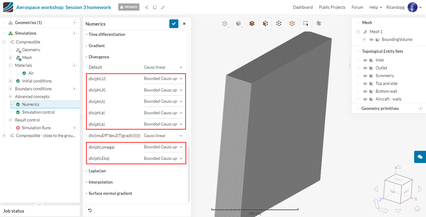
Set the following Divergence schemes to Bounded Gauss Upwind:
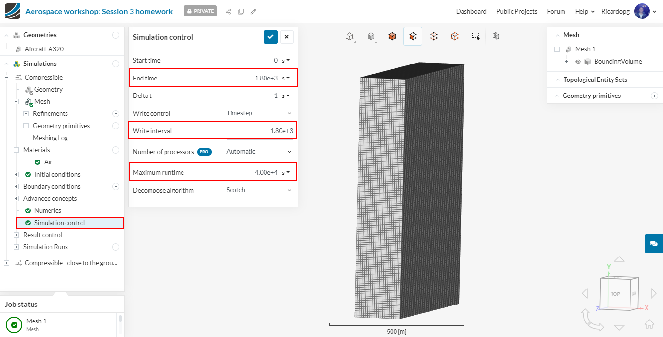
Now, in Simulation control change End time and Write interval to 1800. Raise Maximum runtime to 40000 seconds. The number of processors is automatically determined by SimScale to optimize core hours usage.
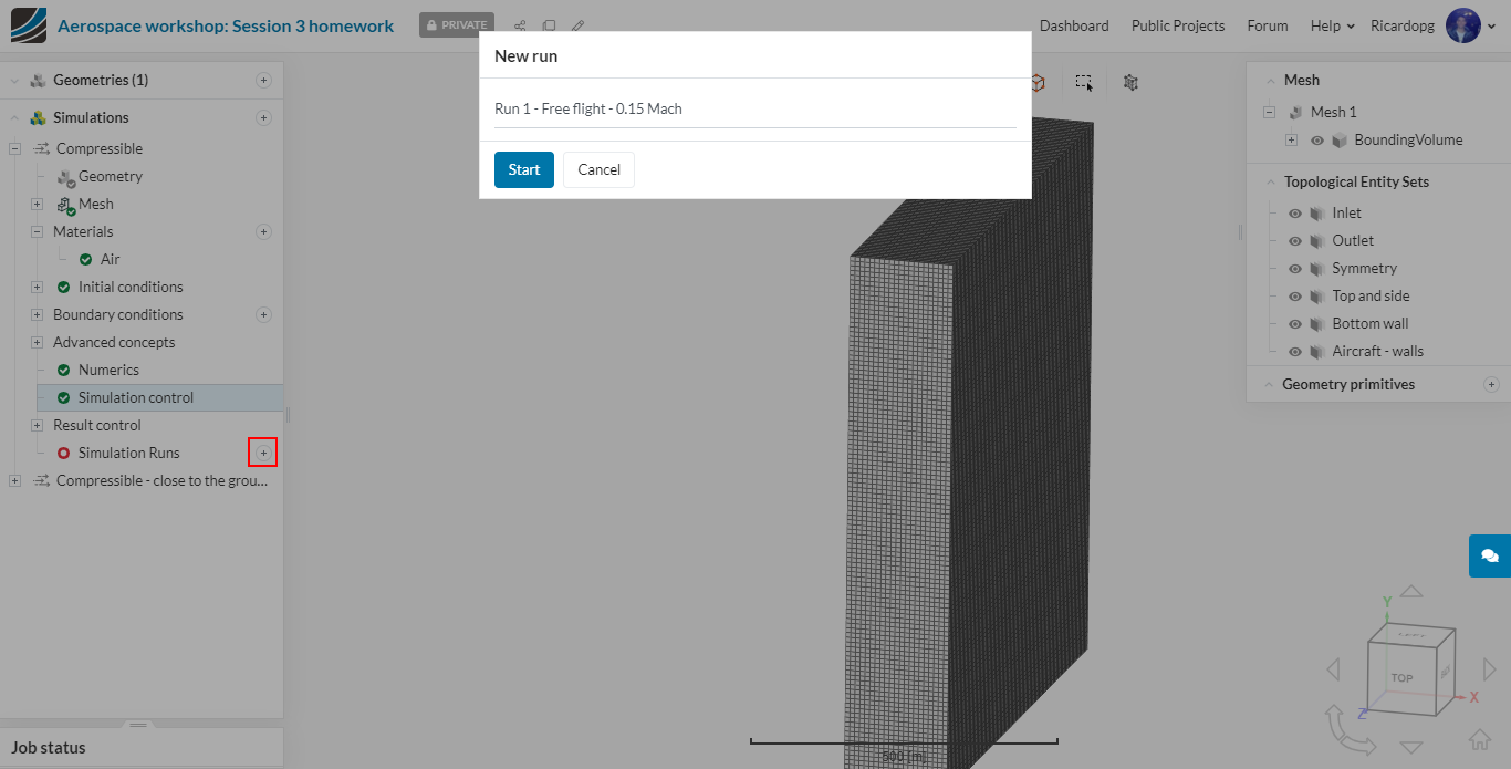
We can now proceed to creating a Simulation Run.
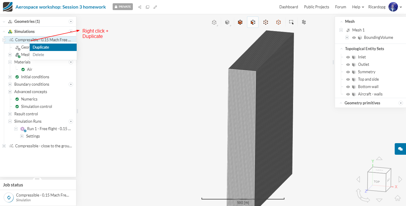
Create new simulations for Mach 0.25 and 0.35 by duplicating the first compressible setup.
Configuring the 0.25 Mach simulation is straight forward. It only requires you to update velocity inlet, k and omega.
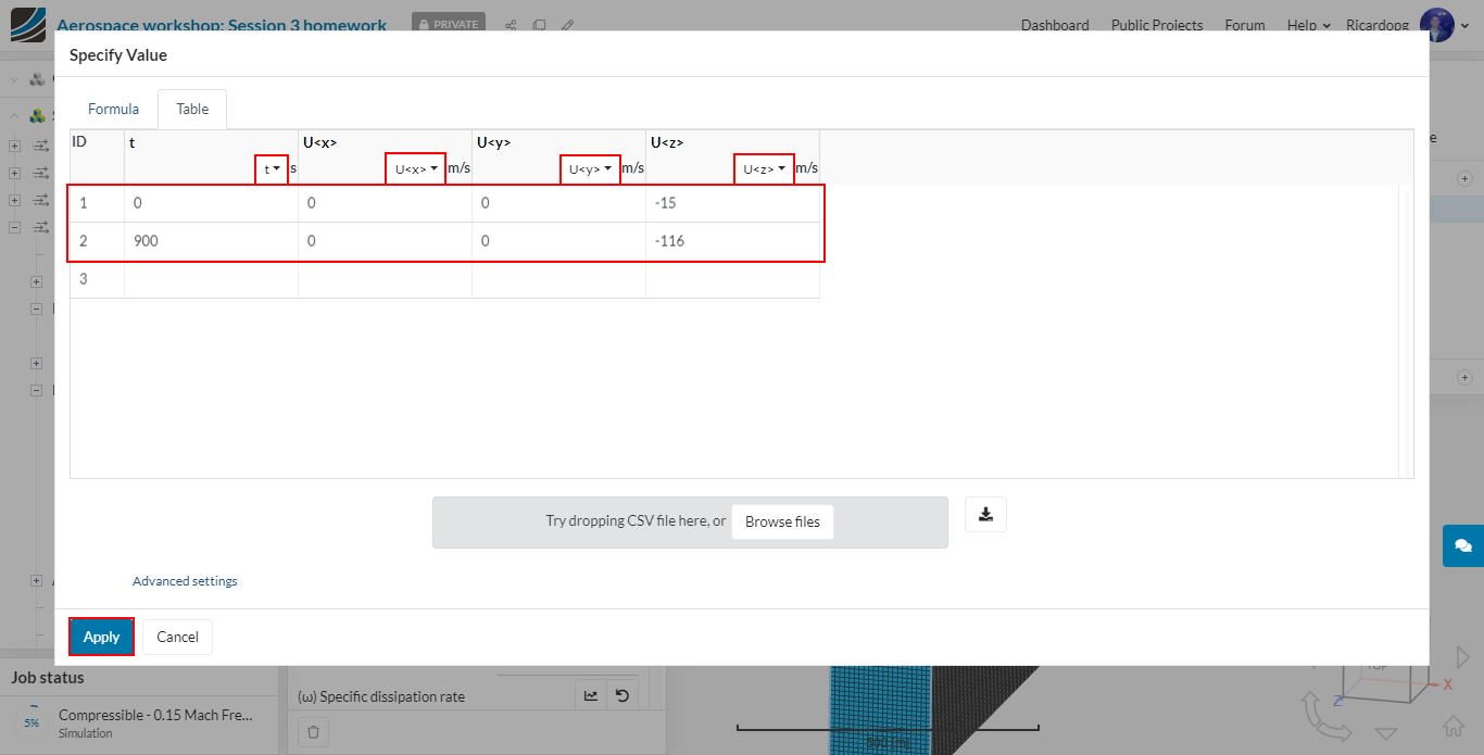
For 0.35 Mach, velocity will be ramped to avoid divergence early on in the simulation. To set up a ramped velocity, do as follows:
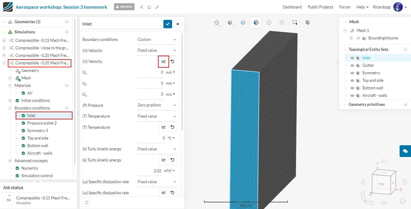
At t = 0 iterations, a velocity of -15 m/s (in Z) will be applied to the Inlet. When the number of iterations reaches 900, the velocity in the Z direction is updated to -116 m/s.
For the Aircraft close to the ground, the set up follows the same logic as the one we just did:
- Go to Topological entity sets and create similar sets for inlet, outlet, symmetry, top-side, bottom and aircraft walls for the new mesh.
- Assign the Material air to the new region.
- Assign the Initial conditions to the domain and Boundary conditions to the new topological entity sets created.
- Duplicate the simulation for new cases using Mach 0.25 and Mach 0.35.
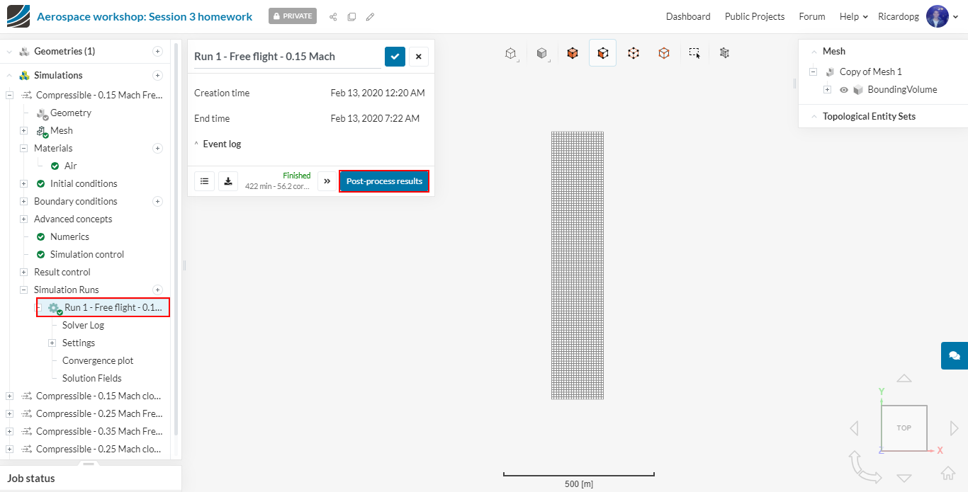
Post-processing
Once the simulation finishes running, click on it and head over to the post-processing environment by clicking on Post-process results
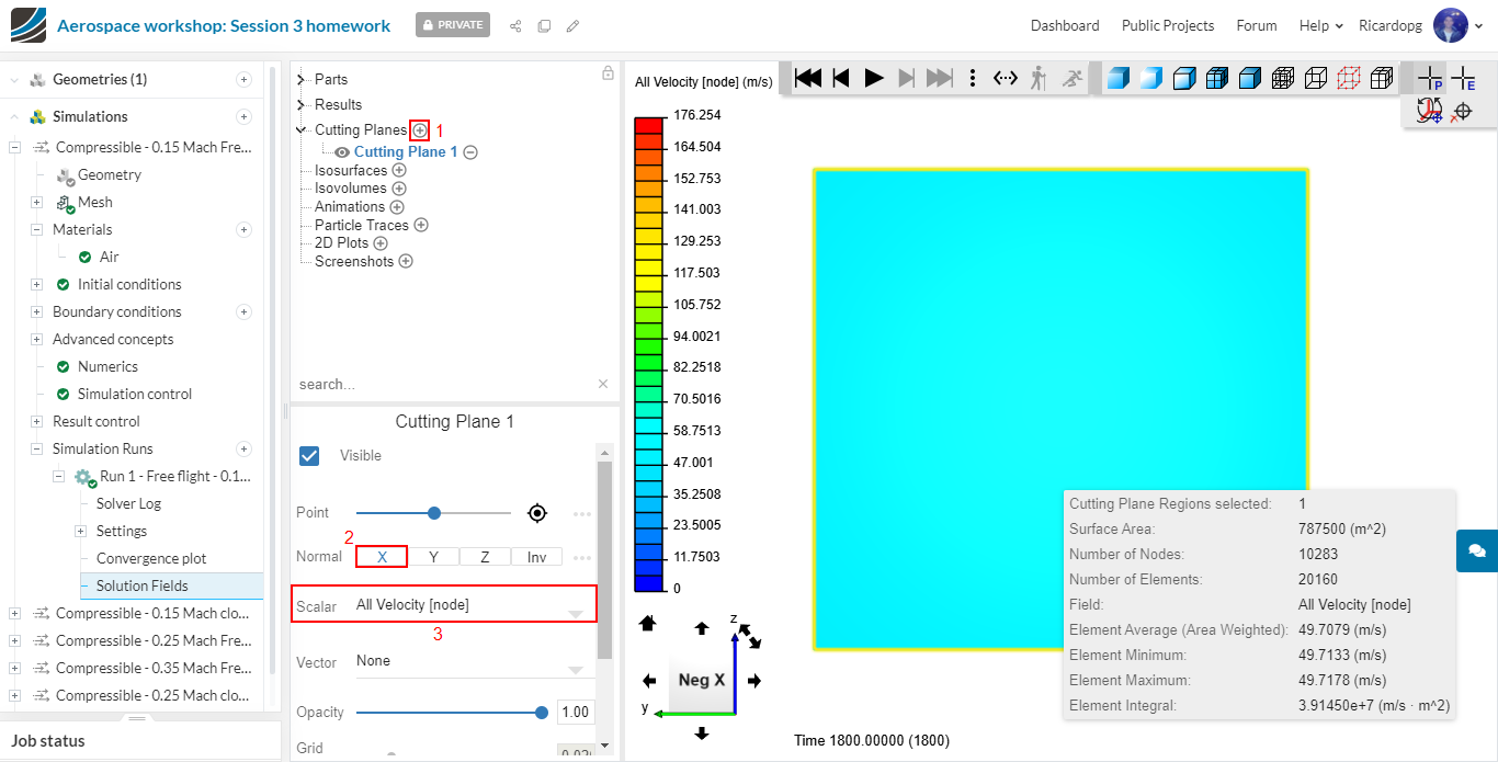
In the post-processing panel, you can find a list of filters and functions. Please click on Cutting Planes to create a slice.
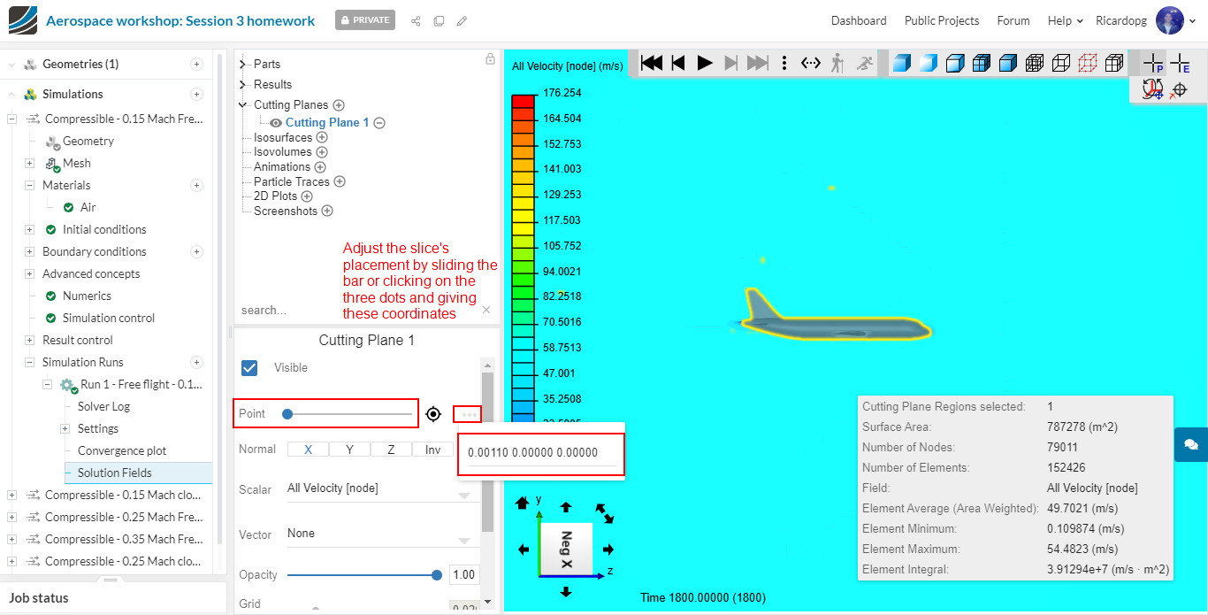
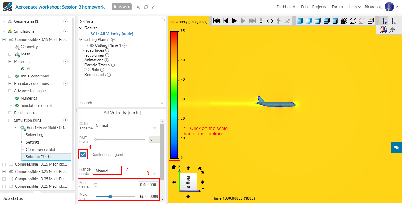
In order to visualize the airplane, the placement of our cutting plane has to be adjusted. This can be done either by the adjusting the sliding bar next to Point or by entering the coordinates 0.0011 0 0 after clicking on the three dots next to the sliding bar.
Click on the scale and adjust the settings to make it represent the data set better:
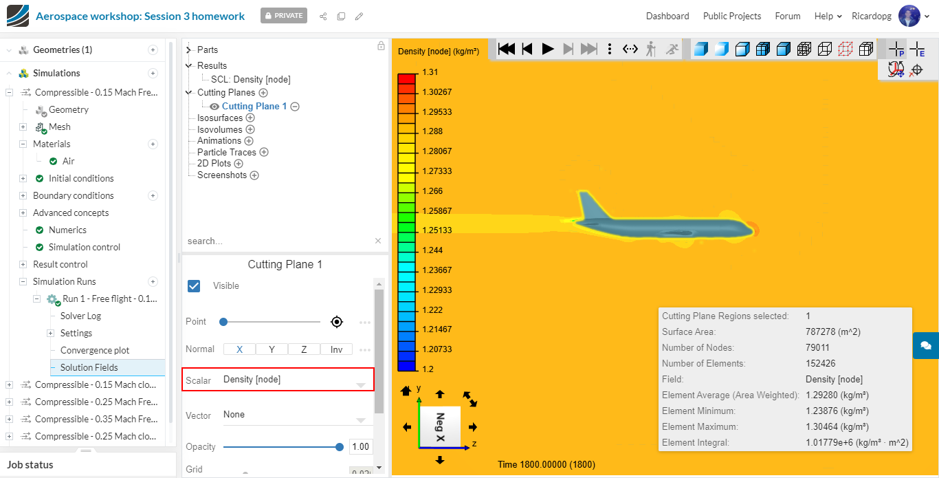
To show density, click on Cutting Plane 1 and change Scalar to Density [Node]. Adjust the scale to the range of 1.2 to 1.31:
Now let’s check the pressure contours on the airplane’s surface. To do this, first delete the previously created cutting plane. Right click in the viewer and select Show all parts.

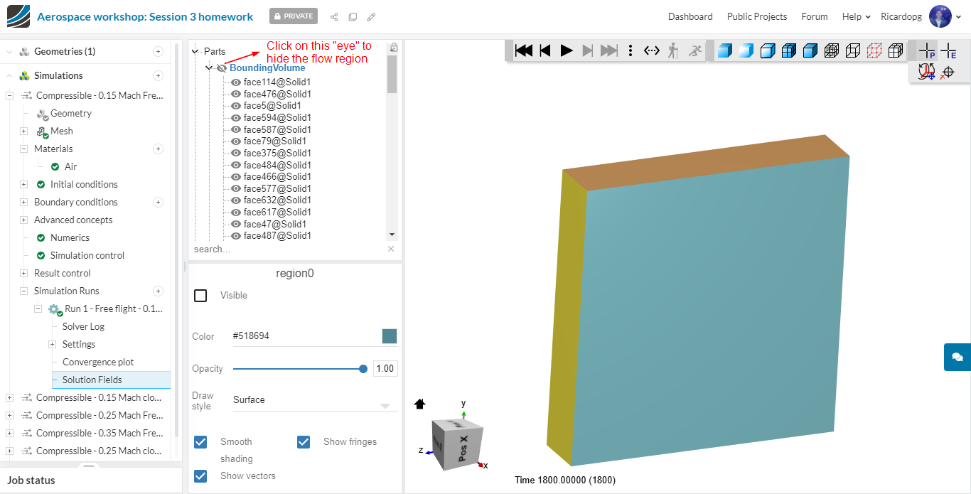
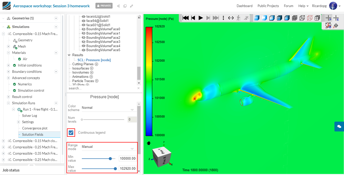
After hiding the flow region, only the boundaries will be shown. Go ahead and hide the Bounding Volume Faces 0, 1, 2 and 3. Then Click on Results and select Pressure [Node]:
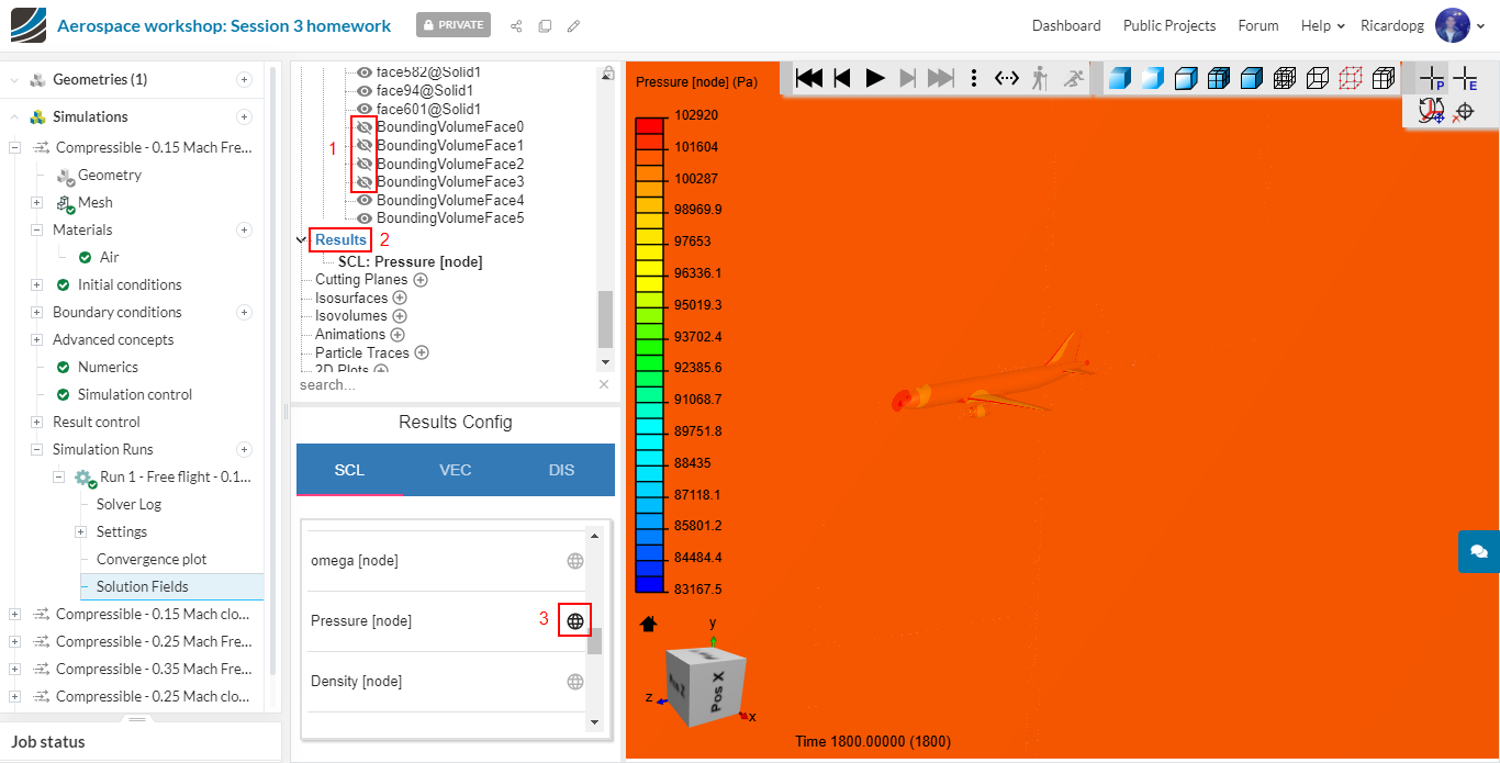
Please adjust the scale’s range from 100000 to 102920 Pa.
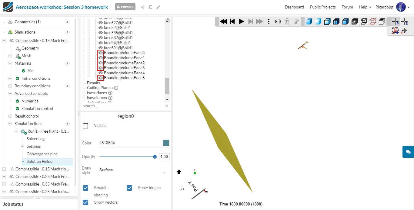
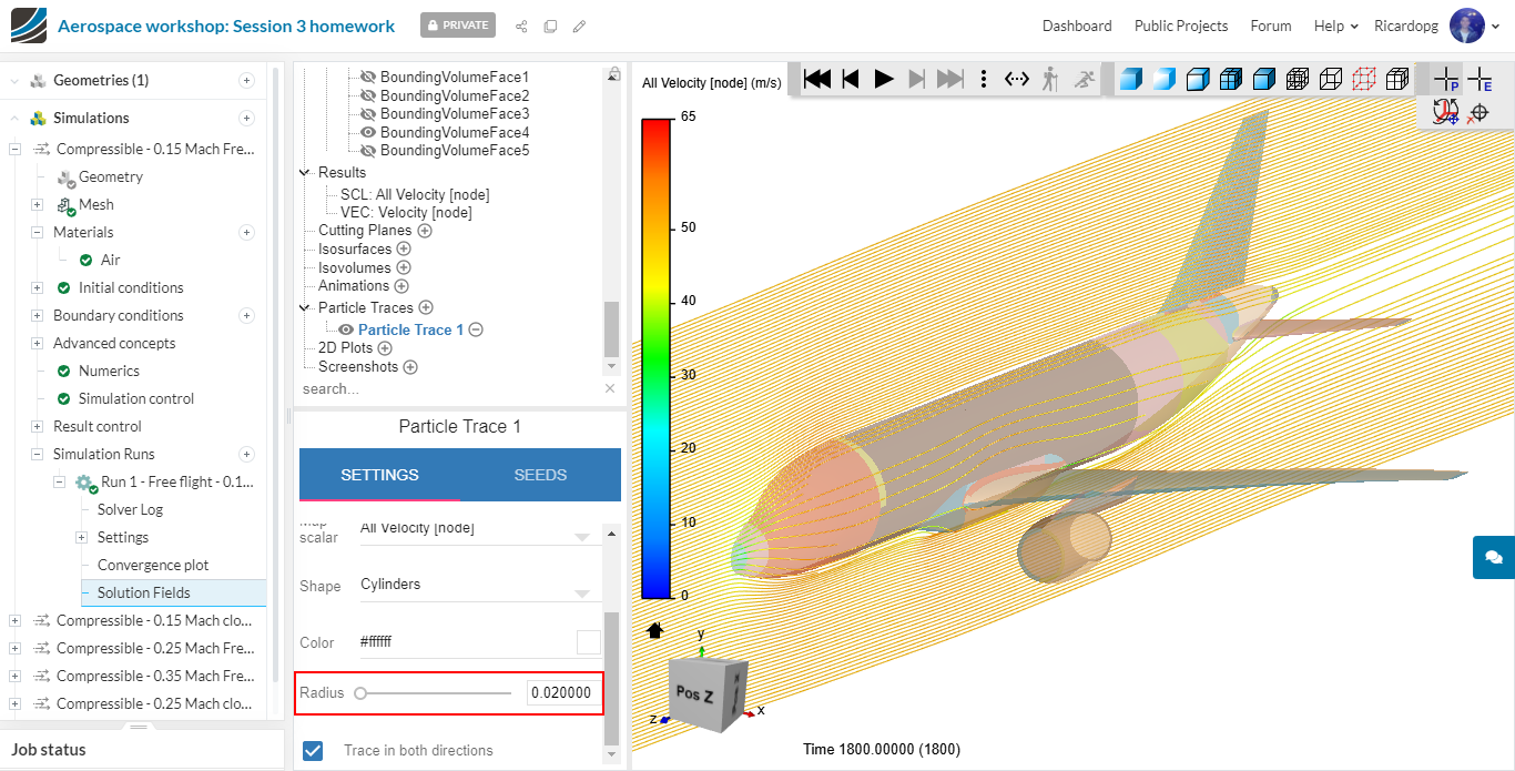
Let’s add Particle traces in order to get the flow streamlines. In the following pictures, the BoundingVolume is still hidden and only the BoundingVolumeFace4 aswell as the aircraft surfaces are being displayed.
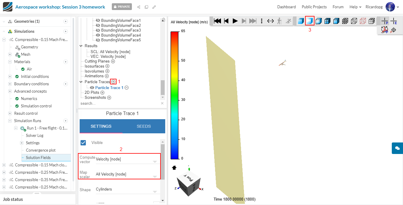
Add a Particle traces and adjust Compute vector and Map scalar to Velocity [node] and All Velocity [node] respectively. Then click on the Transparent surface icon towards the top of the screen to give a nice effect to the walls.
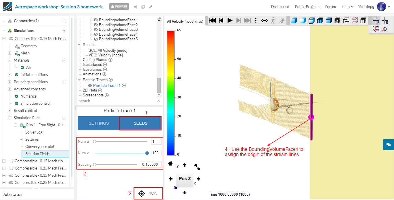
Now, to create a new particle trace, click on SEEDS, then on PICK and select a surface from which the traces will be generated (you can use the bounding volume face to do that). The Radius of streamlines can be adjusted under SETTINGS. The number of streamlines aswell as the spacing between them can be adjusted in SEEDS.
A lot of different particle traces configurations are possible, so we encourage you to play with the settings and get other cool pictures.
Now, for the other simulation runs, perform similar post-processing and compare!