Recording

Homework Submission
For your homework, your task is to setup a steady-state structural analysis of an aluminum front suspension upright and analyze the results for stress and deformation.
The step-by-step tutorial below contains all of the steps for setting up the simulation in SimScale and visualizing the results.
To submit your homework assignment, please generate a public link of your project (Sharing a Project)
Homework Deadline: Sunday, December 17th, 11:59 pm CET
Click Here to Submit your Homework
Outline
PART 1:
-
Introduction
-
Project Import
-
Mesh Generation
a. Automatic Meshing -
Simulation Setup
a. Domain
b. Material
c. Boundary Conditions
d. Numerics
e. Simulation Control
f. Simulation Runs -
Post-Processing
a. Filters/Visualization
b. Additional Features
Introduction
The purpose of an upright assembly is to provide a physical mounting and links from the suspension arms to the hub and wheel assembly, in addition to carrying brake components. It is a load-bearing member of the suspension system and is constantly moving with the motion of the wheel.
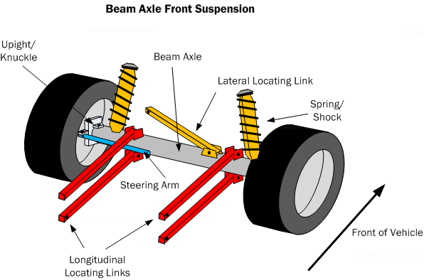
Image credit: http://www.buildyourownracecar.com/
For the upright assembly on an FSAE car, the design goal is to provide a lighter design that does not compromise in terms of both stiffness and performance. Finite Element Analysis can be used to ensure that the upright design is adequate and will not fail during the racing competition.
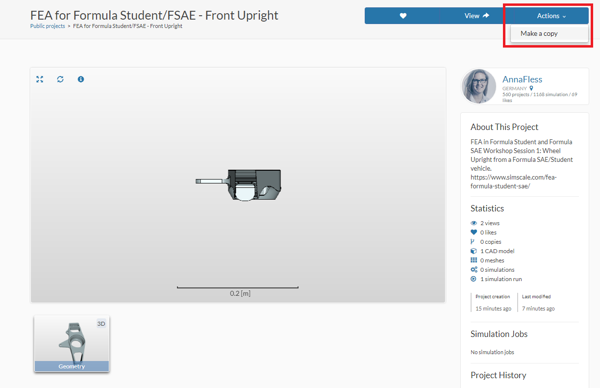
Project Import
To start this exercise, please click on the link below and then make a copy of the project.
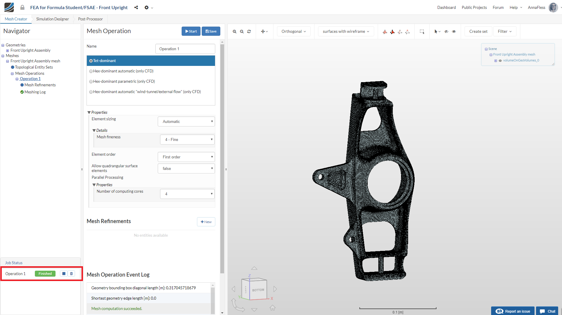
Mesh Generation
In the Mesh Creator tab, click on the geometry Front Upright Assembly
Then, click on the New Mesh button in the options panel.

Select Tet-Dominant mesh and select the following parameters - Automatic for Element Sizing, 4-Fine for Mesh fineness, First order under the Element order, and 4 for Number of computing cores.
This operation will automatically create a mesh for the geometry. The cell size and refinement will be adapted automatically.
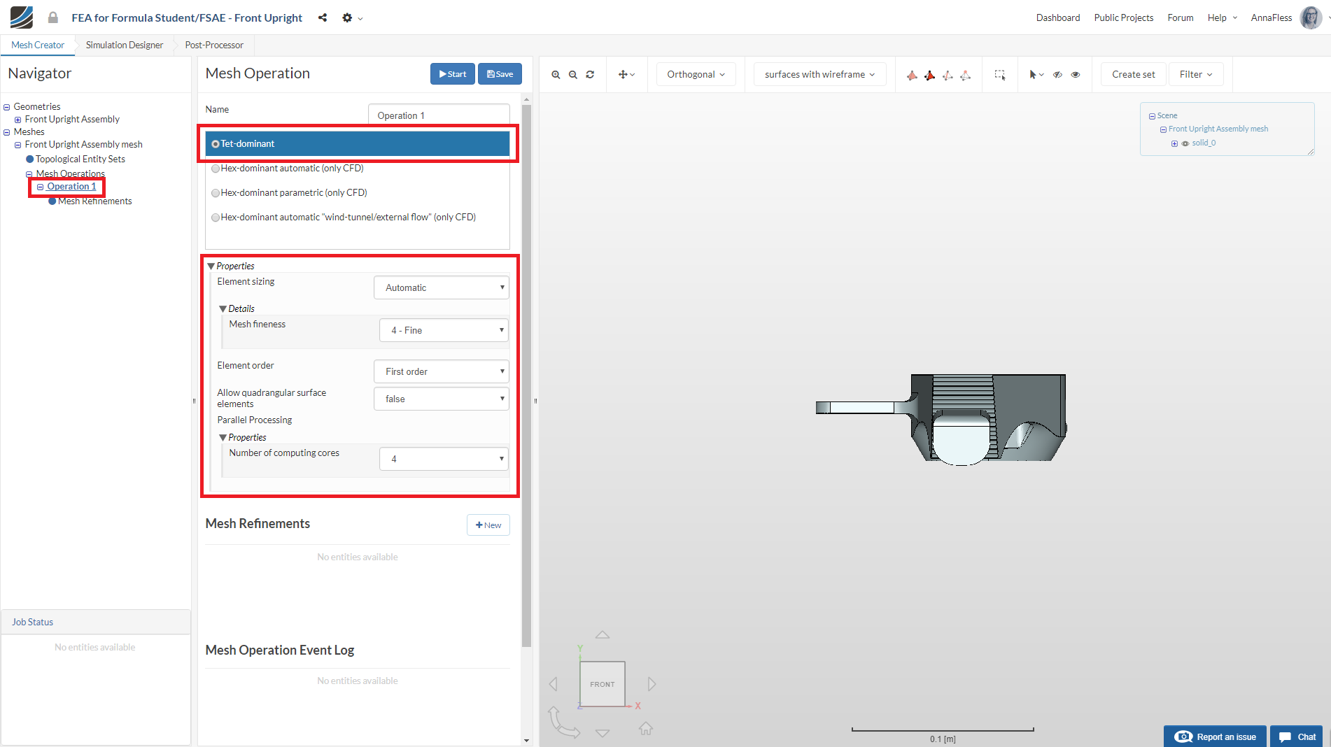
Click on the Save button to save all settings.
Now click the Start button to begin the mesh operation. The meshing job will start in a few moments. You can see the status of the mesh in the bottom left corner of your screen.
The mesh operation takes about 5 minutes to complete.
Simulation Setup
For setting up the simulation switch to the Simulation Designer tab and select New simulation.
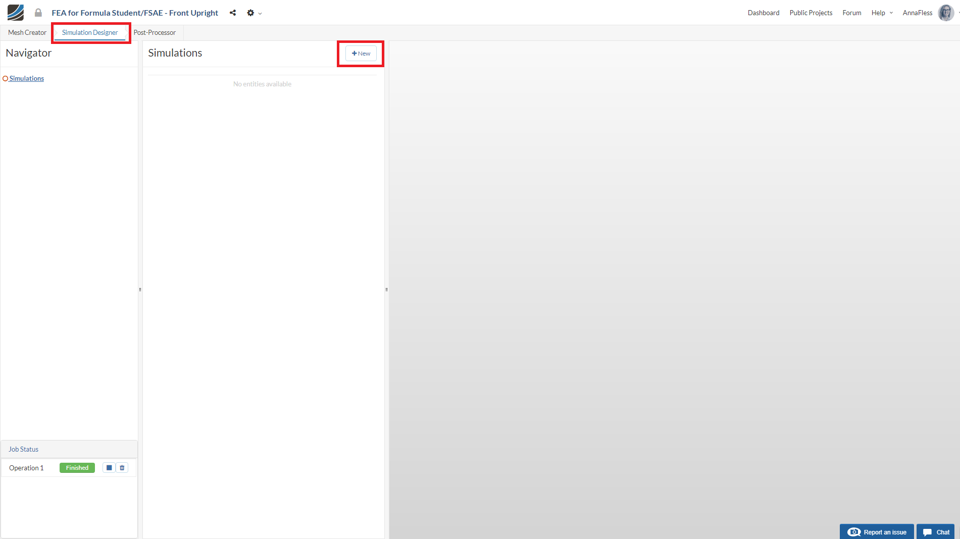
A pop-up window will appear allowing you to choose the analysis type for the simulation. Since our load will be static and deformations will be relatively small, select the analysis type Static under Solid mechanics and click create.
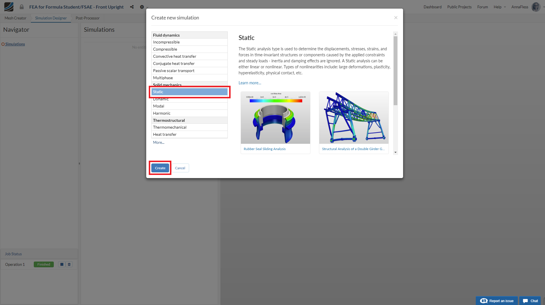
Leave the Nonlinear analysis option set to false.
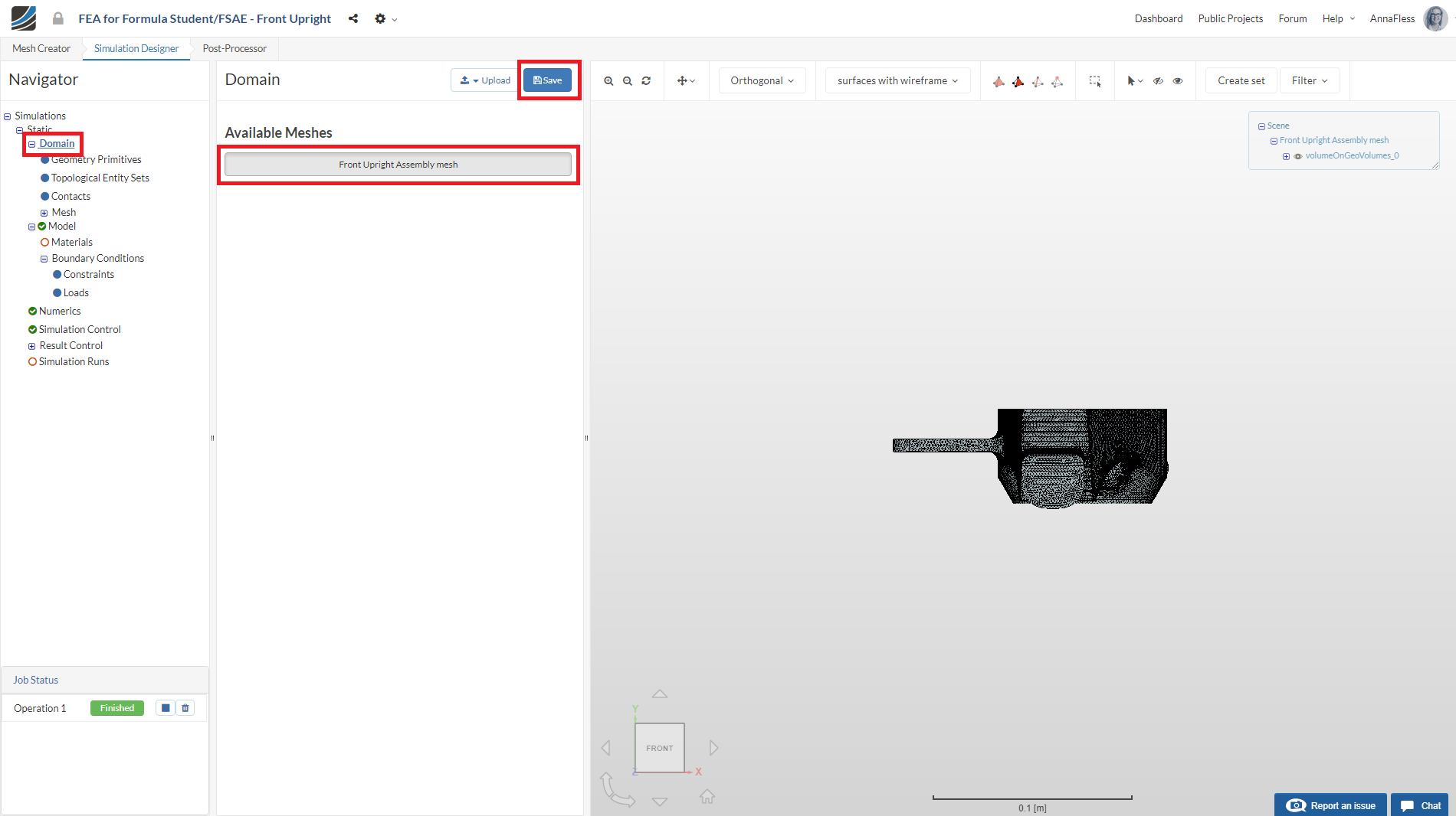
Domain
The green check marks on the items in the Navigator refer to saved states whereas the red entries denote fields with missing data that must be filled in.
Click Domain from the tree and select the mesh that you created. Click the Save button. The mesh will then automatically load in the viewer.
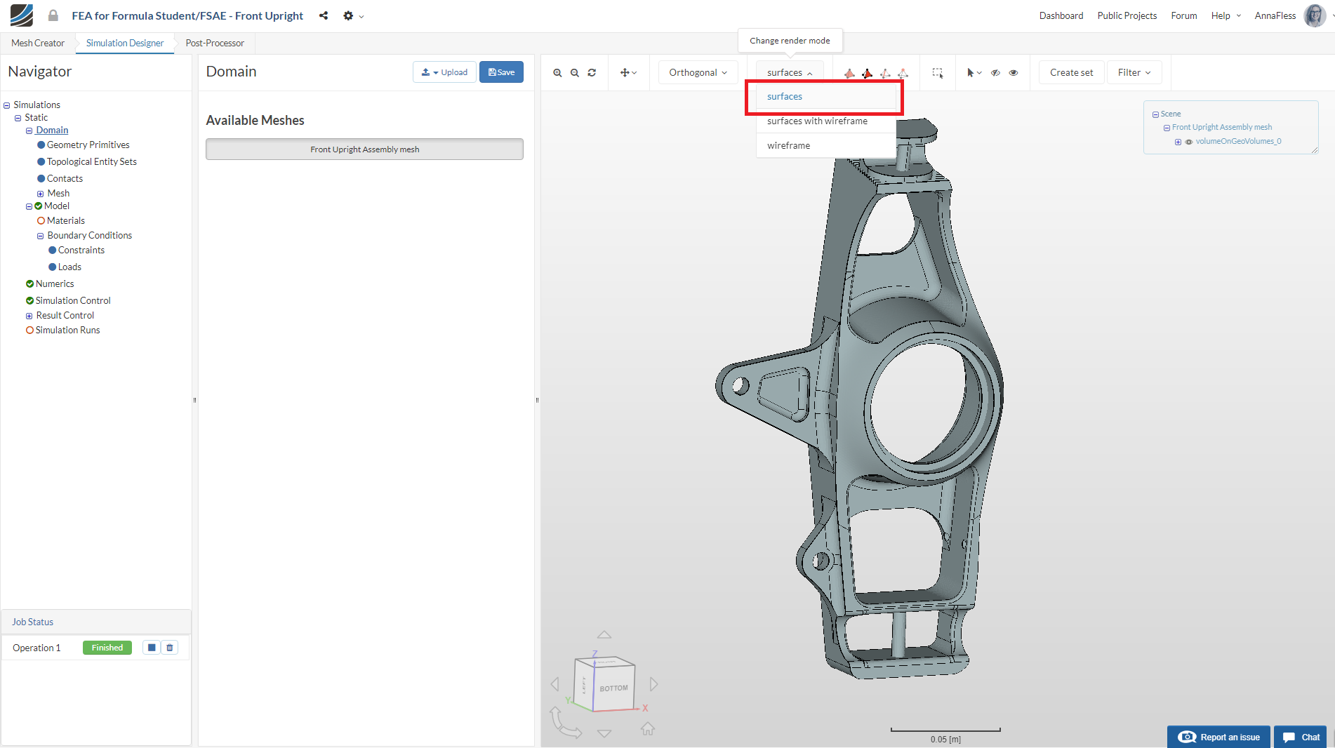
Change the render mode to Surfaces to interact with the mesh more easily.
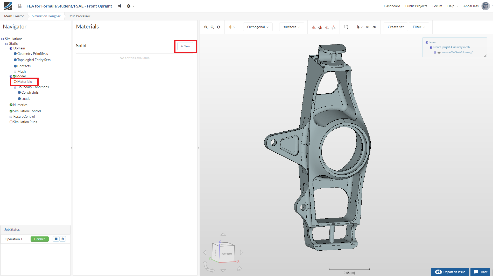
Select Solid Material
Now we will define the material for the front upright. Select Material in the Navigator and click New.
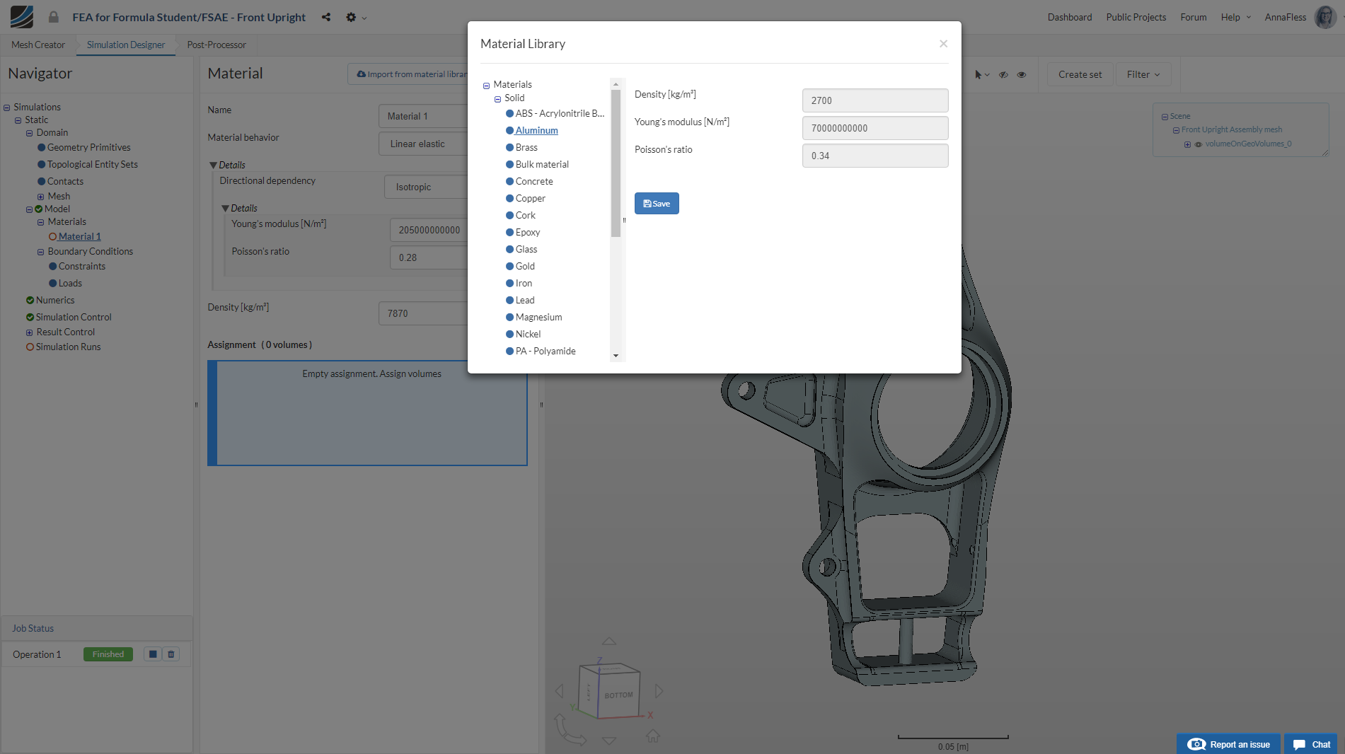
Click on Import from material library to import the desired material from the material database.
Select Aluminum and click Save.
Click on your model in the viewer. You should now see the entire Volume assigned under Assignment
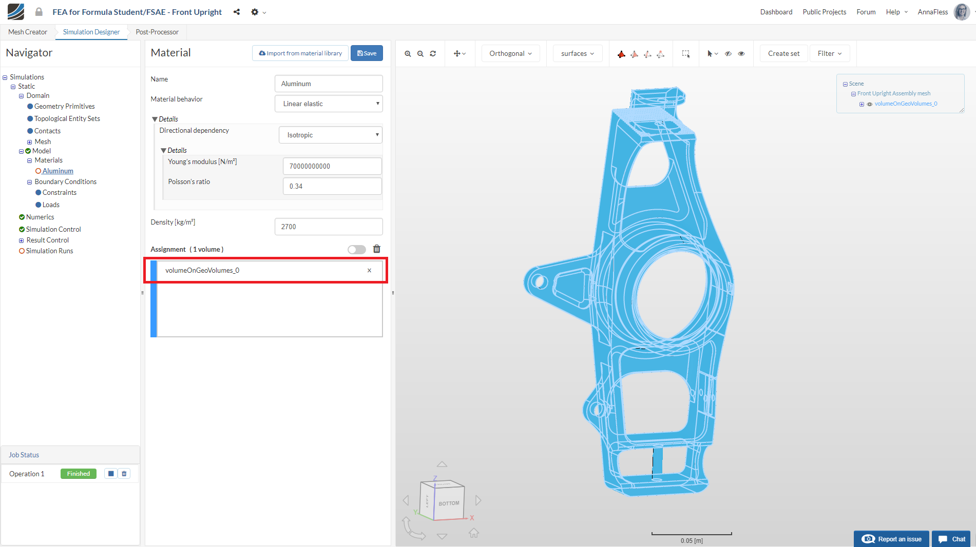
Click Save in order to define the material for this region.
Boundary Conditions
In this section, we will define the constraint (fixation) and loads for our simulation case. This is one of the most important parts of the simulation set-up. Boundary conditions are how we tell the solver how the part behaves in a physical sense.
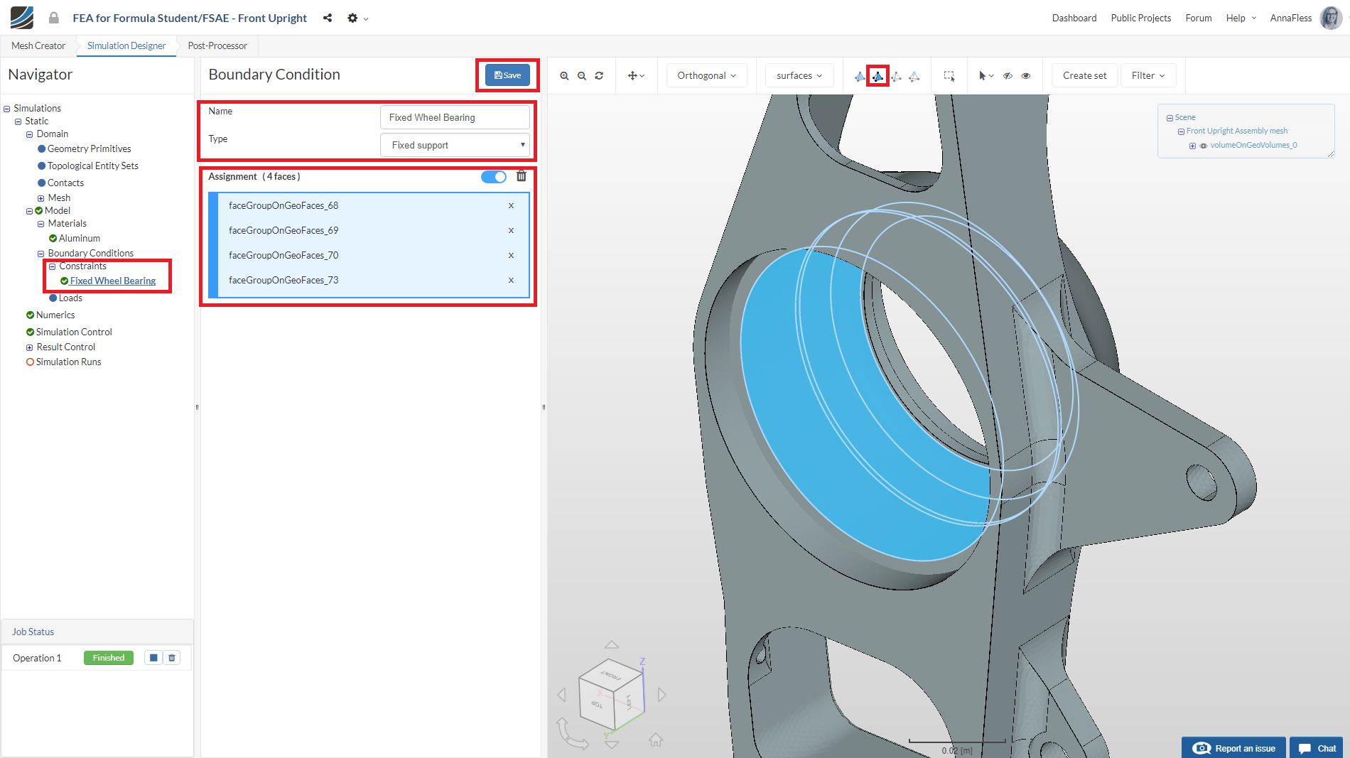
Let’s first define the fixation. Select Constraints in the tree and click New.
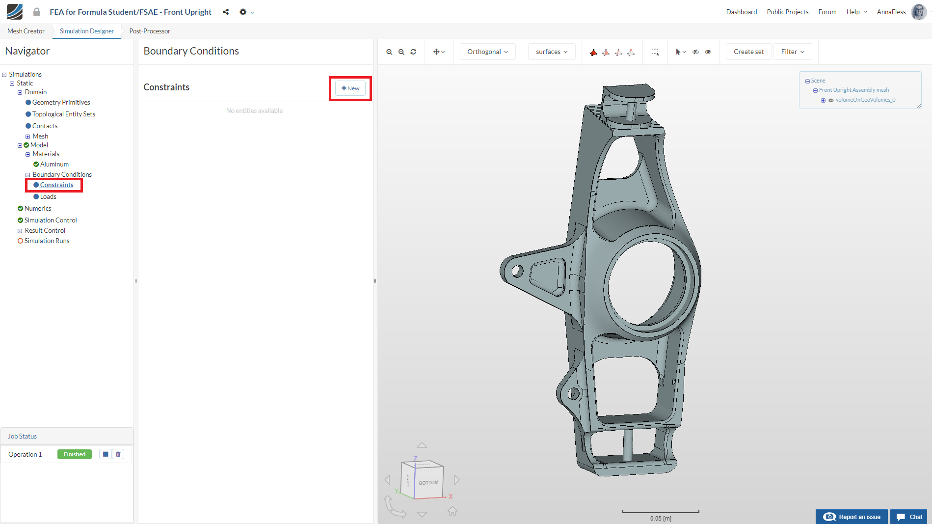
A new boundary condition with default name will be created. Rename it to Fixed Wheel Bearing.
Under Type select Fixed Support.
Assign the Boundary Condition to the four faces of the wheel bearing as shown in the image below and click Save.
Next, we will define the loading Boundary Conditions. Select Loads in the tree and click New
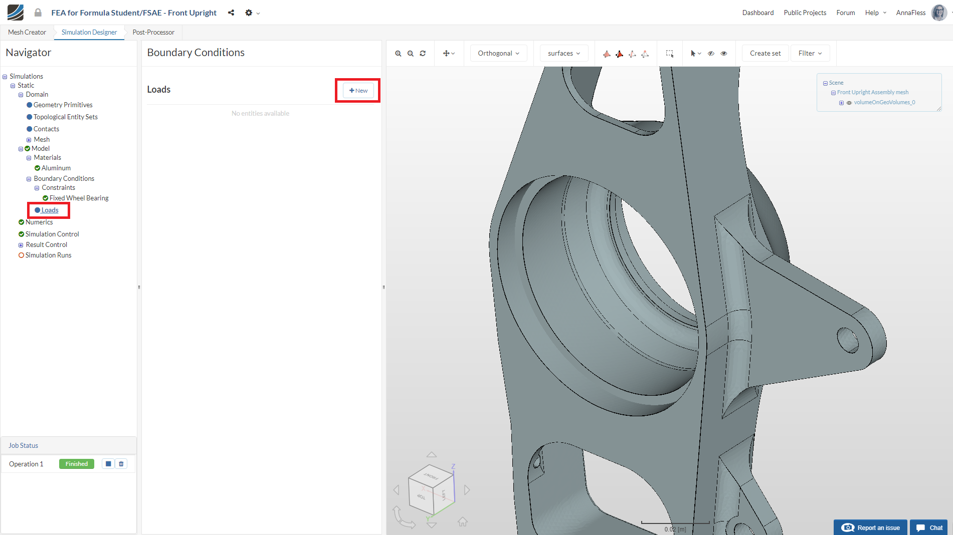
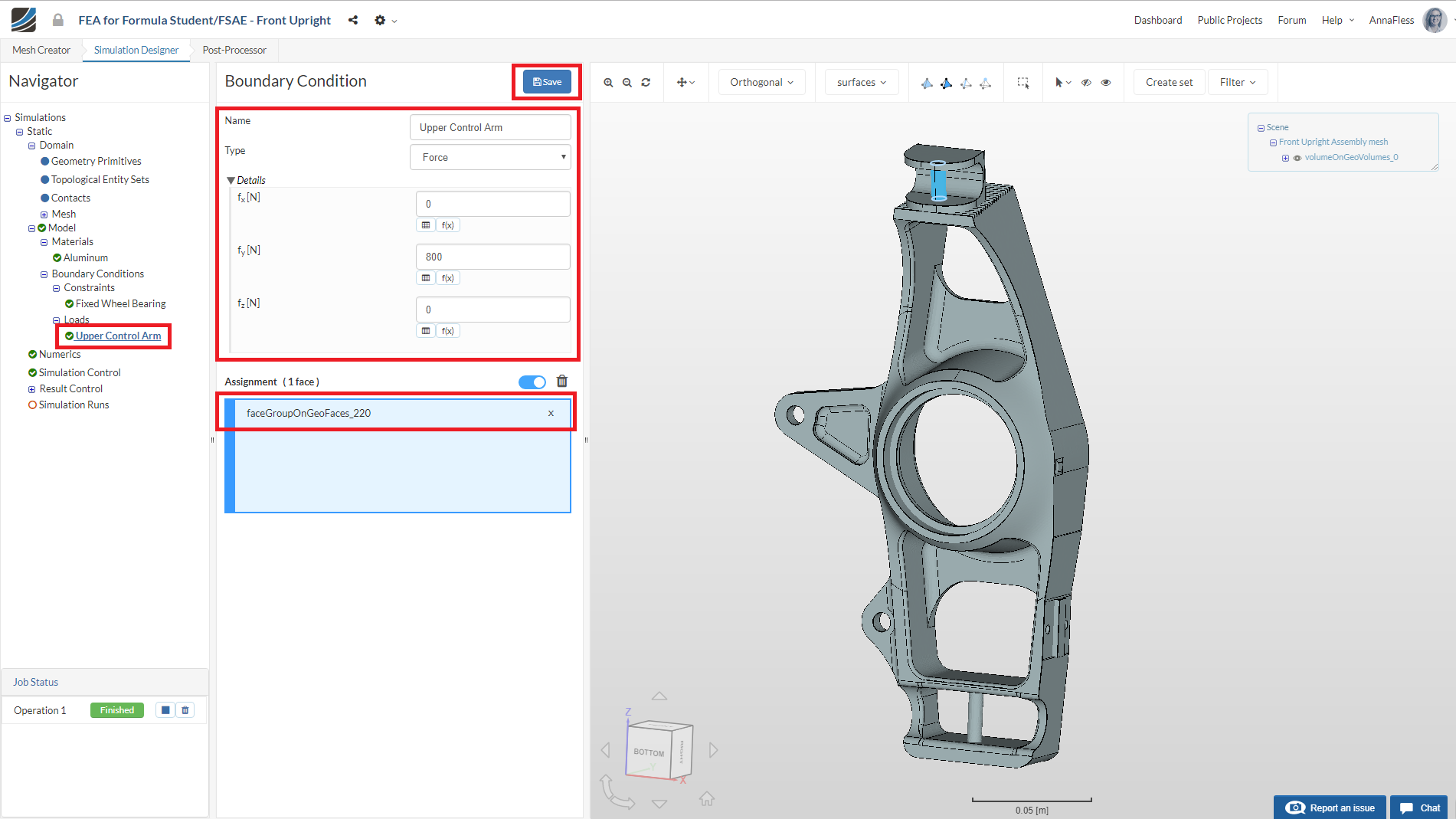
A new boundary condition will be made under Loads. Rename it to Upper Control Arm
Set the Type to Force and apply the a load of 800 N in the fy direction.
Assign the load to the face of the upper cylinder and Click Save.
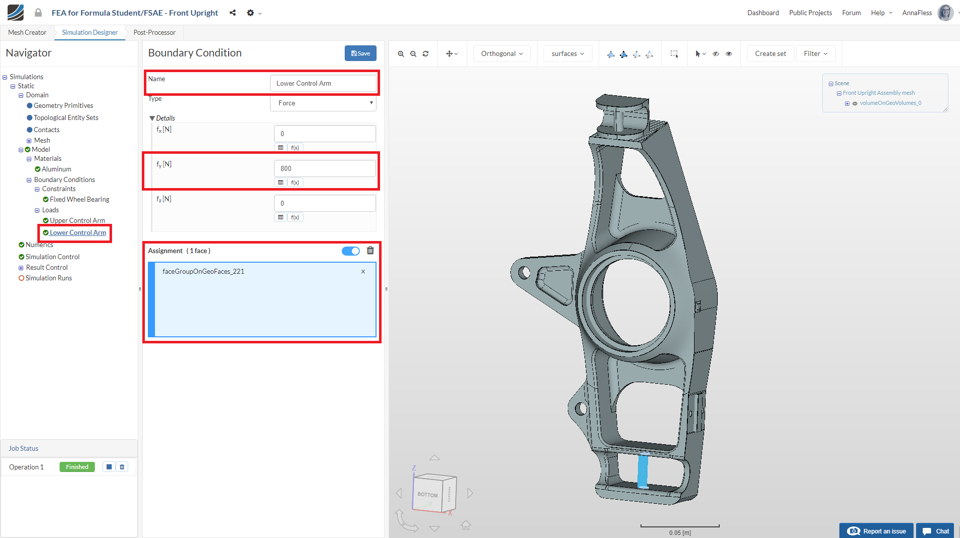
Next, we will assign the same load to the face of the lower cylinder. Select Loads in the tree and click New
A new boundary condition will be made under Loads. Rename it to Lower Control Arm
Set the Type to Force and apply the a load of 800 N in the fy direction.
Assign the load to the face of the lower cylinder and Click Save.
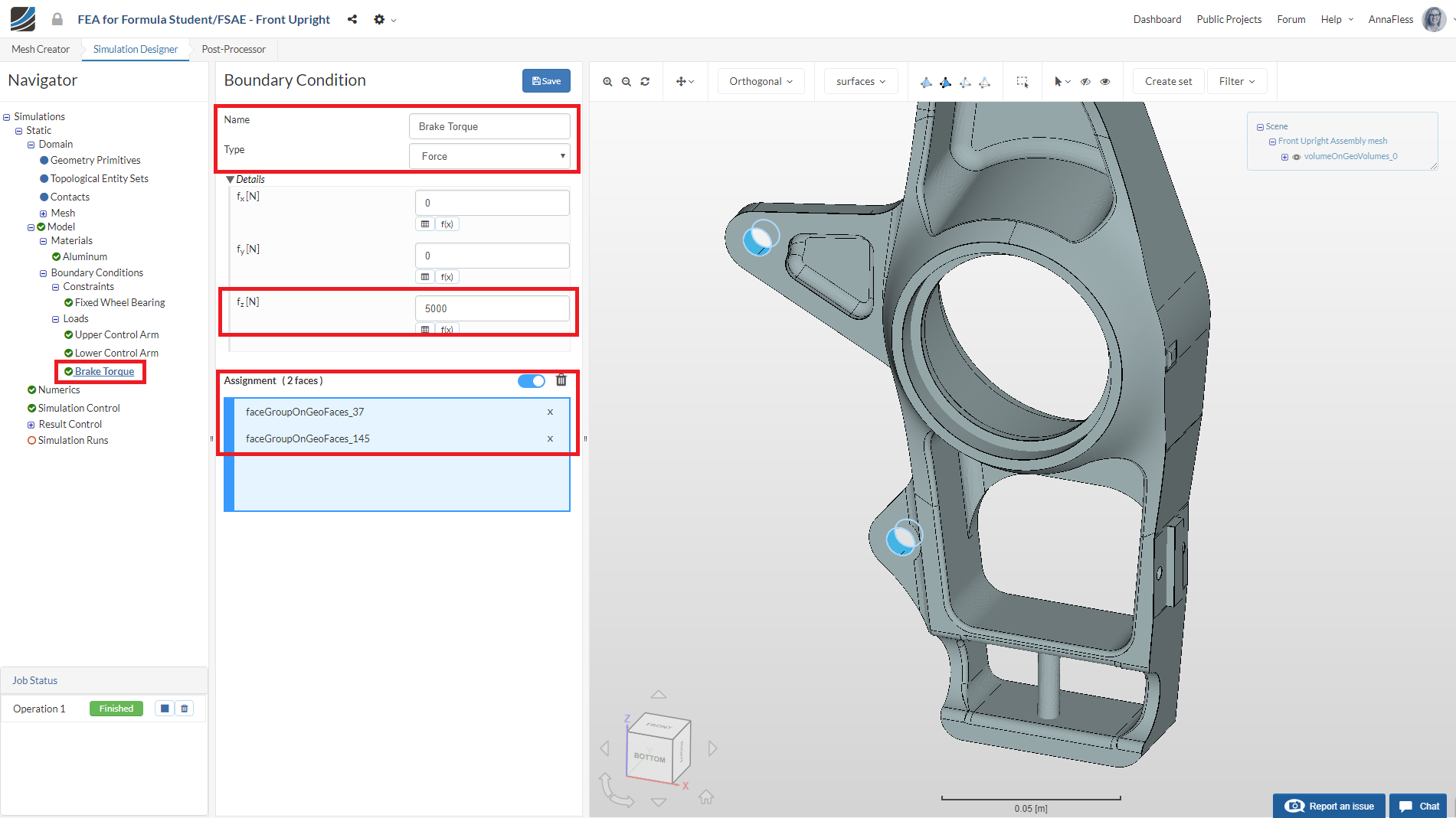
The third and final load that we will assign is for the brake torque. Select Loads in the tree and click New
A new boundary condition will be made under Loads. Rename it to Brake Torque
Set the Type to Force and apply the a load of 5000 N in the fz direction.
Assign the load to the two faces where the brake would attach to the upright assembly and click Save.
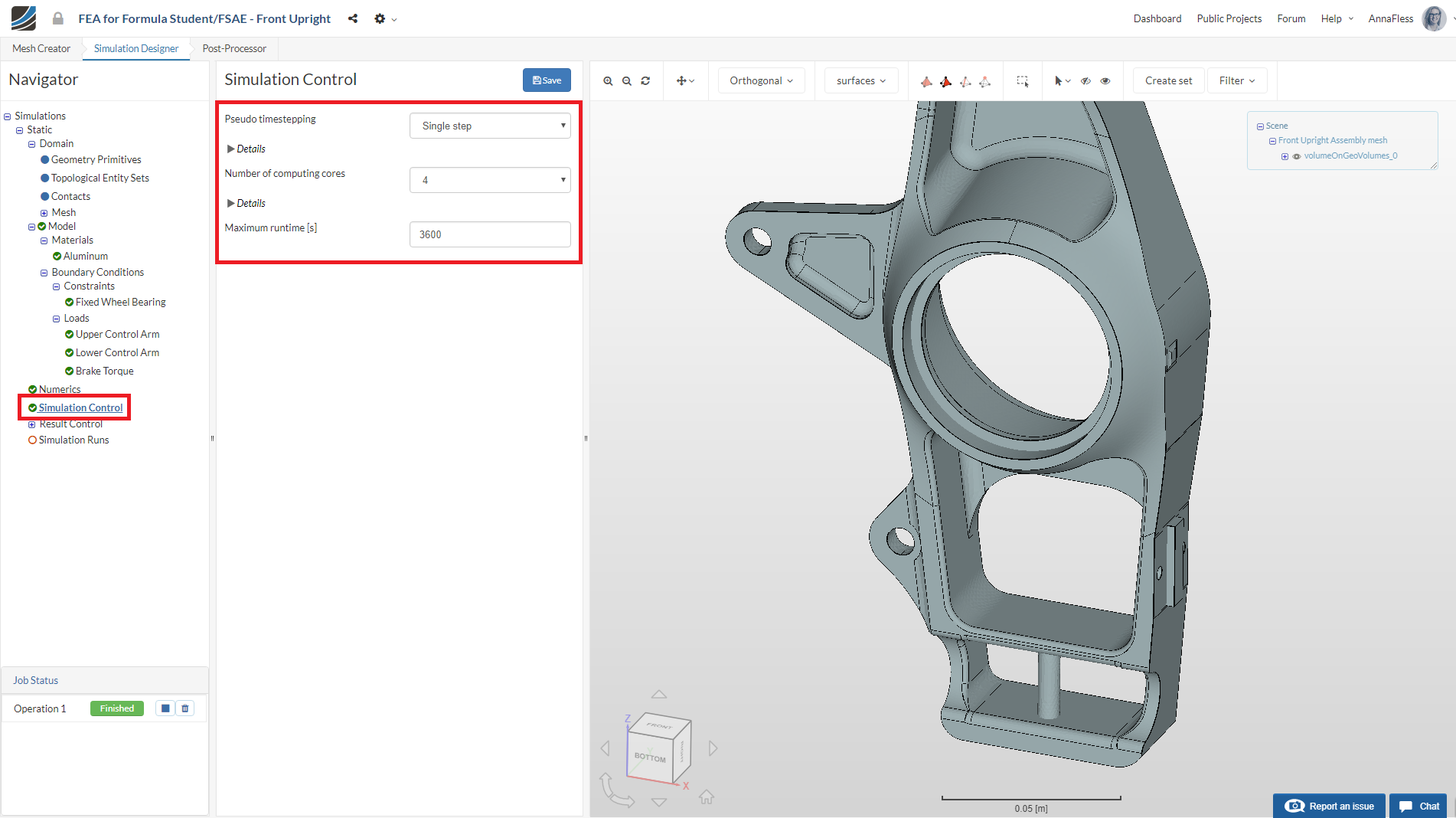
Simulation Control
Next we will move to the Simulation Control item in the project tree to define the parameters we want to use to run the simulation.
Click on Simulation control. Since we are doing a linear static analysis, the applied load does not vary based on time and the inertial and damping forces are ignored. This means that we can set up and run our simulation under a single timestep
The number of computing core needed to run a simulation is highly dependent on the size of the model (number of nodes). In this case, 4 computing cores is sufficient.
Leave the maximum runtime set to the default value of 3600 s. This parameter rarely needs to be changed for static simulations due to the low computing power required.
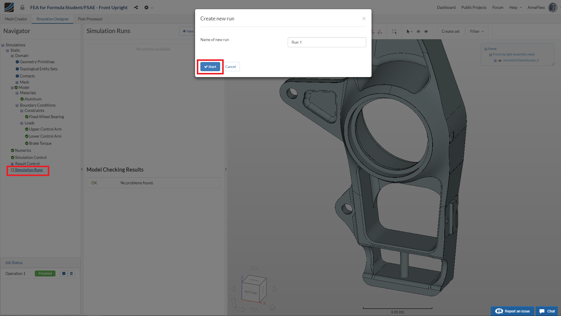
Create New Run
Click on Simulation runs and create a new run by clicking on New.
The final step is to click Start. Your simulation is now computing in the cloud.
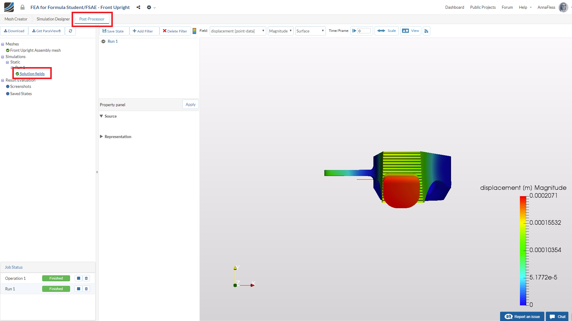
Post-processing
Once the simulation is finished (this will take about 4 minutes), go to the Post-processor tab to view the results.
Select Solution fields of Run 1
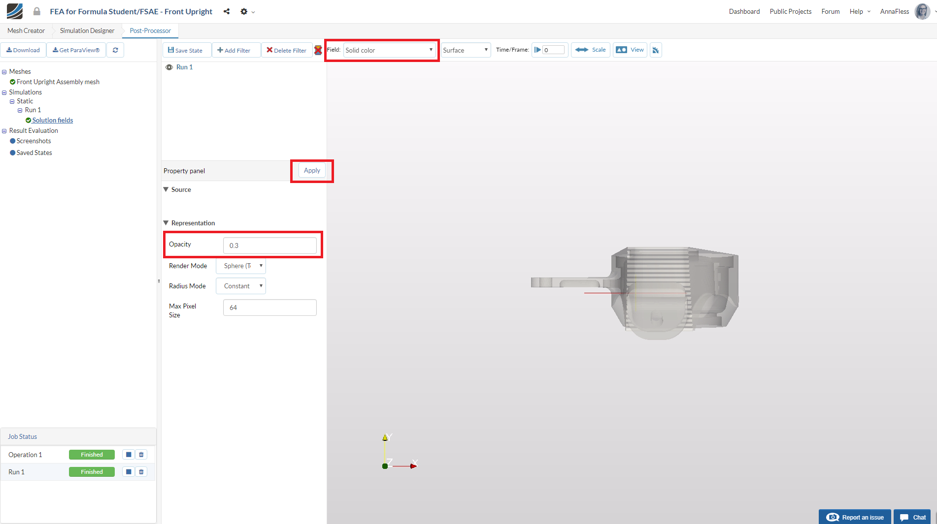
In order to differentiate between the deformed and undeformed geometry of the upright, set the field (at the top left corner) to Solid color and change the Opacity to 0.3. Click Apply. This will make the part a little transparent.
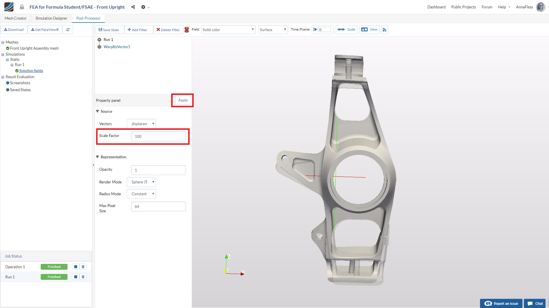
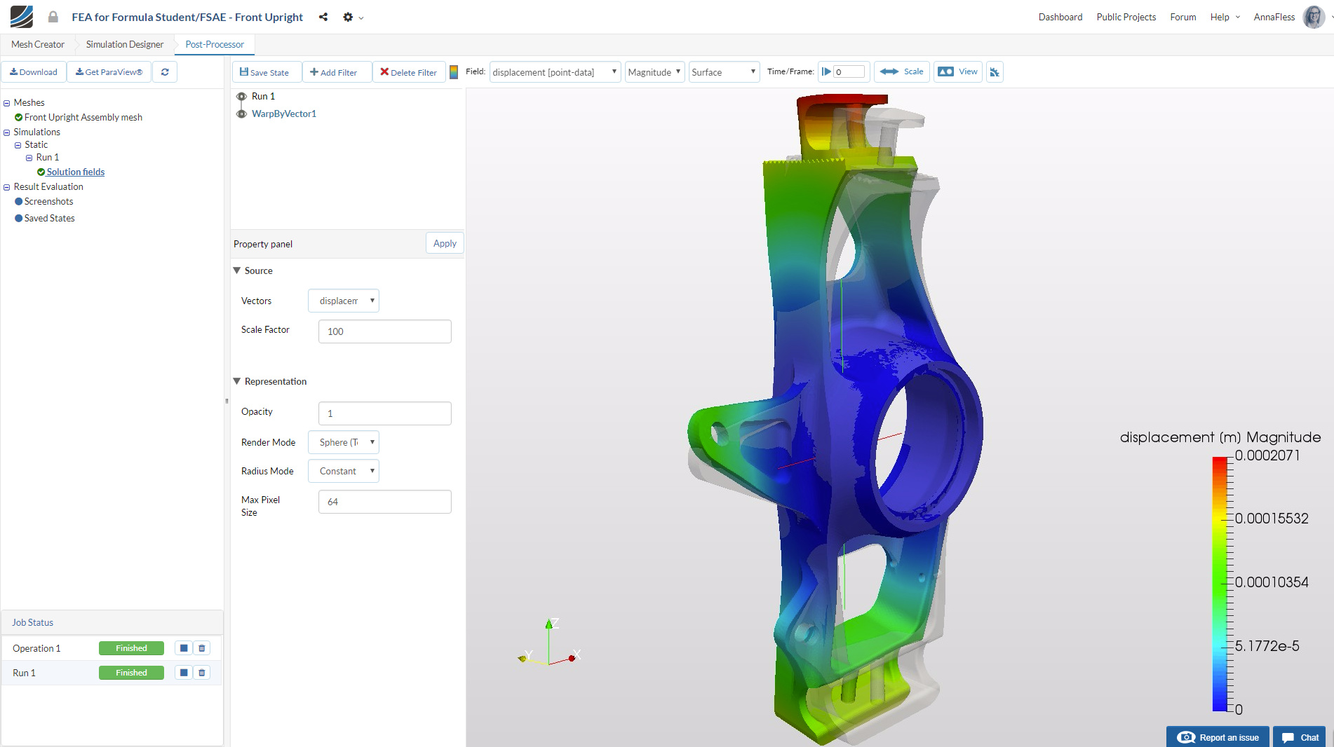
To see the deformed geometry, click on Add Filter and then Warp by Vector. You will see a Warp by Vector filter is added under your solution field and in the result viewer.
The actual deformation of the aluminum upright should be very small. To better visualize the direction of deformation, we can introduce a Scale Factor of 100
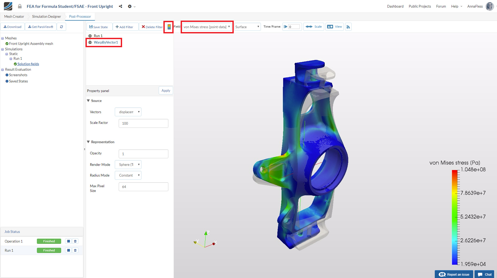
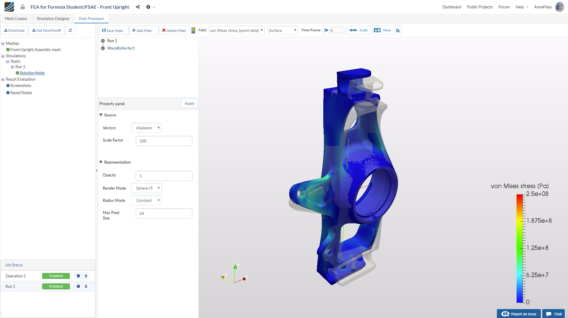
To view the VonMises stress, change the Field to von Mises Stress [point data]. Select the Toggle color bar to view the magnitude of the von Mises stress (right side of the Delete Filter button).
Click on Scale and set the custom data range from 0 to 250e6 Pascals (the upper value in this range is the yield stress of aluminum - or the stress that the material will start to fail.)
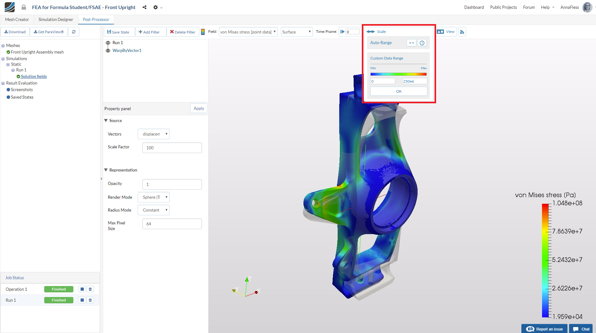
The von Mises stress is now scaled as shown in the picture below:
Click camera icon under Viewport Tools to generate a screenshot. The screenshot will appear under Screenshots section of a Result Evaluation tree item.
Similarly, you can change the fields in the viewer to view the displacements, strain, etc.
Homework Submission
To submit your homework assignment, please generate a public link of your project (Sharing a Project)
Homework Deadline: Sunday, December 17th, 11:59 pm CET