Recording
Aerospace Workshop feat. EUROAVIA (Session 1) ― Ventilation of Aircraft Cabin
Exercise
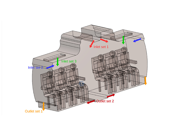
This exercise involves simulating the ventilation inside an aircraft cabin. For simplicity and reduced computation there is only one row of seats in the geometry. The task is quite interesting, to setup 6 different configurations by having various configurations of inlet and outlet, and then to compare the results. The possible inlets and outlets are as shown in the following figure.
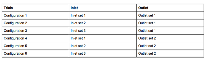
The different combinations for performing the simulations are:
Step-by-Step
Import the project by clicking the link below. ( Crtl + Click to open in a new tab )
Click to Import the Homework Project
Once the project is imported, the workbench is automatically opened. Then follow the steps below for setting up an incompressible flow simulation .
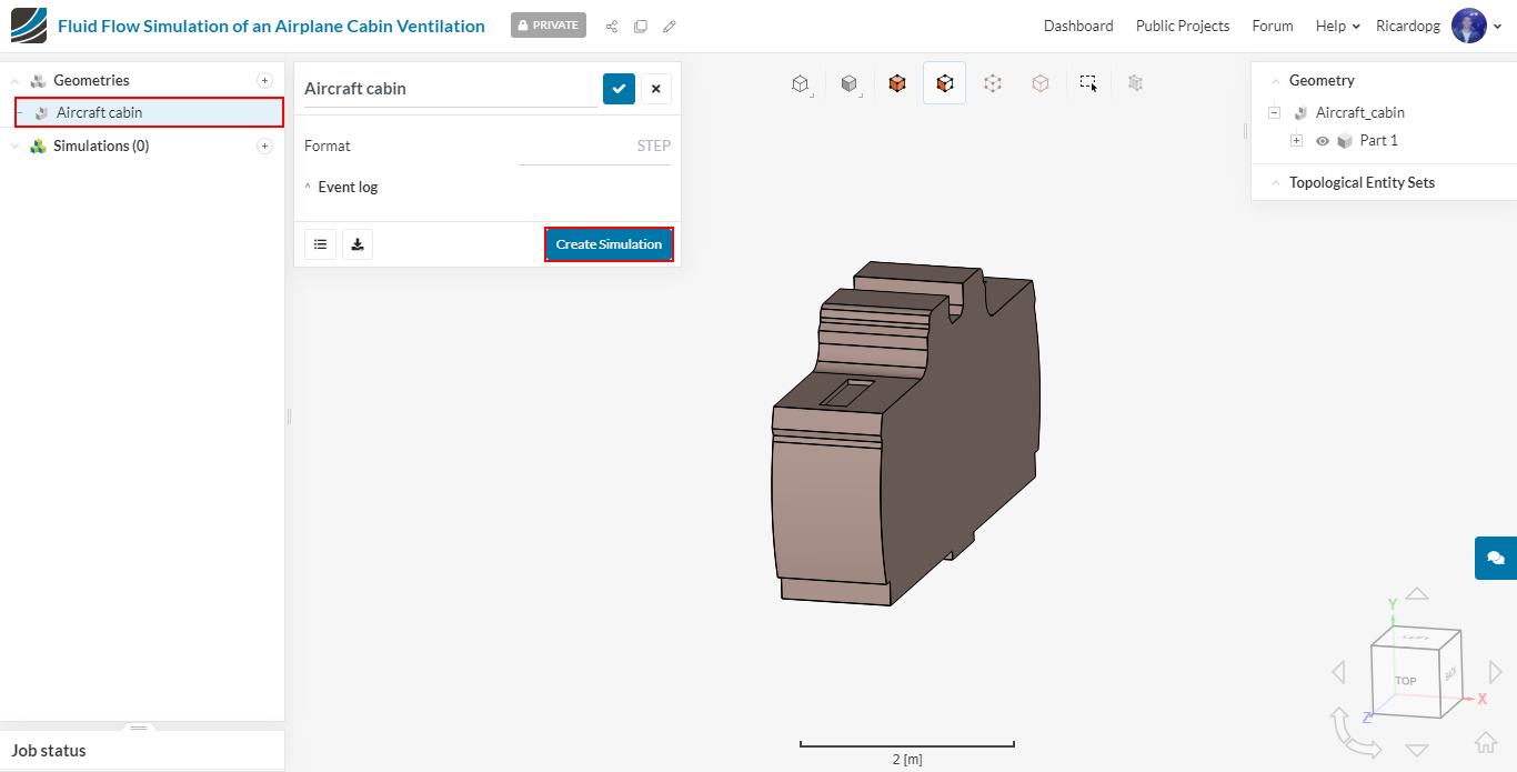
First, click on the geometry named Aircraft cabin and select Create Simulation.
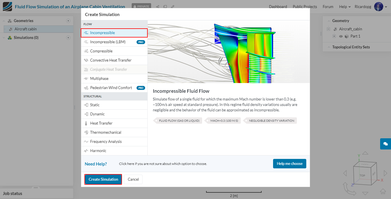
We want to perform an Incompressible analysis. Then go ahead and click on Create Simulation one more time:
Make sure k-omega SST is selected as Turbulence model and Time-dependency is set to Steady-state.
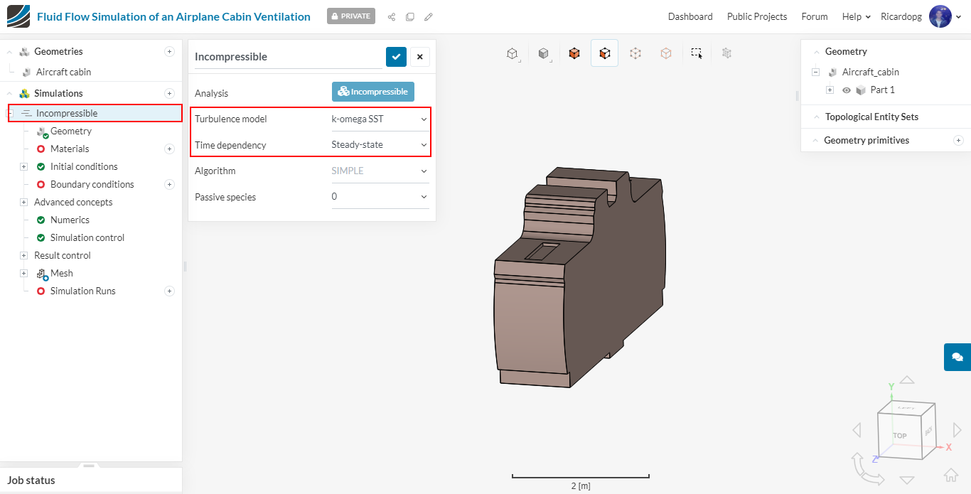
The panel in the left-hand side of screen is often called simulation tree or workflow. In contains several entries that need to be properly filled in order to run the simulations. Entries highlighted in red have missing information, whereas entries highlighted in green have all the information necessary. You can still, of course, edit green entries with more appropriate inputs if need be.
Meshing
In the simulation tree, navigate to Mesh. Change the Algorithm to Hex-dominant (Only CFD) and Fineness to Very coarse. We will add a boundary layer refinement in the next step, so also disable Automatic boundary layers
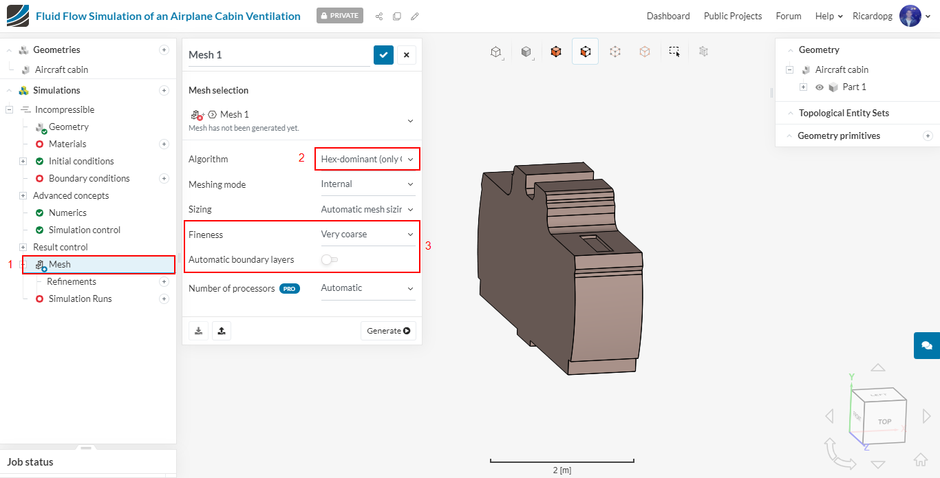
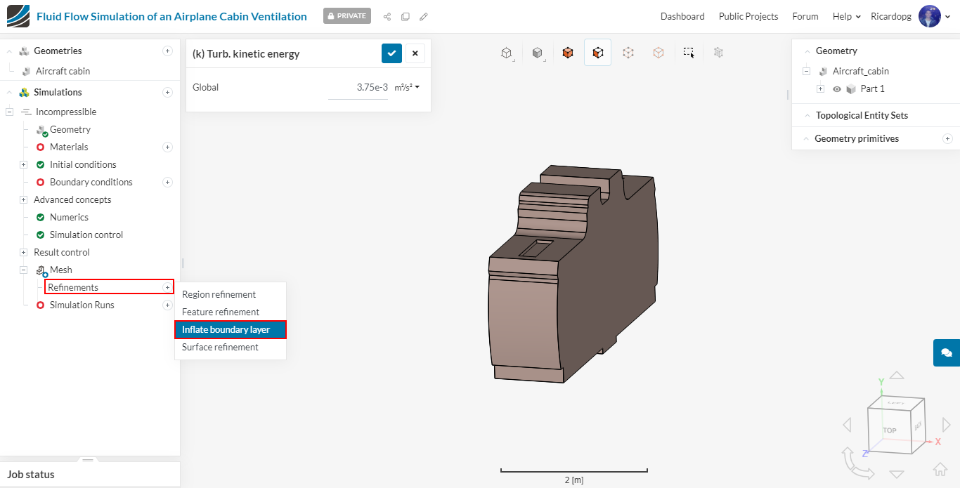
You don’t have to worry with the Number of processors that will be employed. SimScale automatically chooses an optimal number based on the job size. Now let’s add a Refinement. Under Mesh, click on Refinements and select Inflate boundary layer. Settings will be default:
Now please right click in the viewer and select Assign all faces. Then, unselect both symmetry planes as shown in the following pictures:

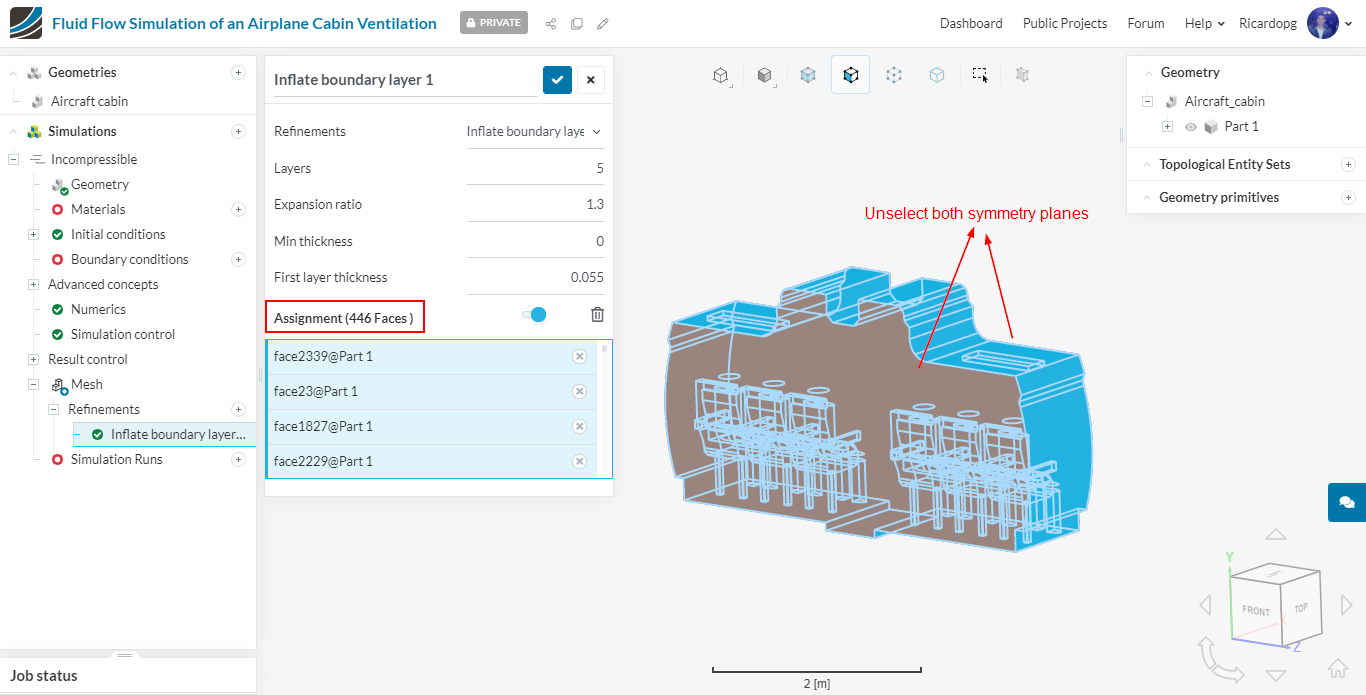
After saving this refinement, we can go back to Mesh and click the Generate button:
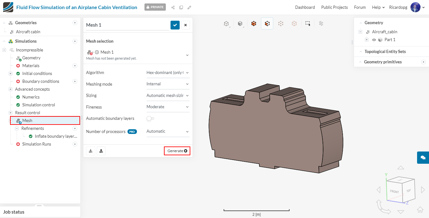
The mesh takes about 35 minutes to be generated. Meanwhile, you can continue working on the setup.
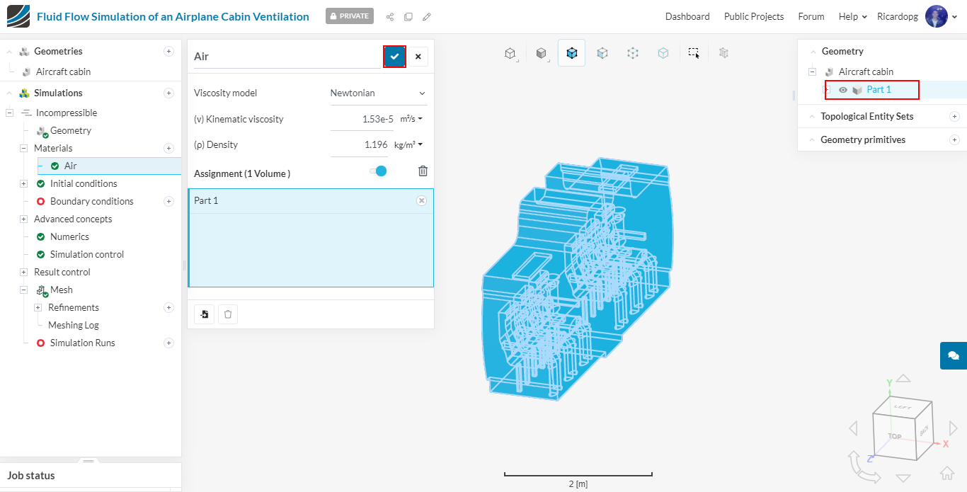
In the simulation tree, navigate to Materials. Select Air and Apply
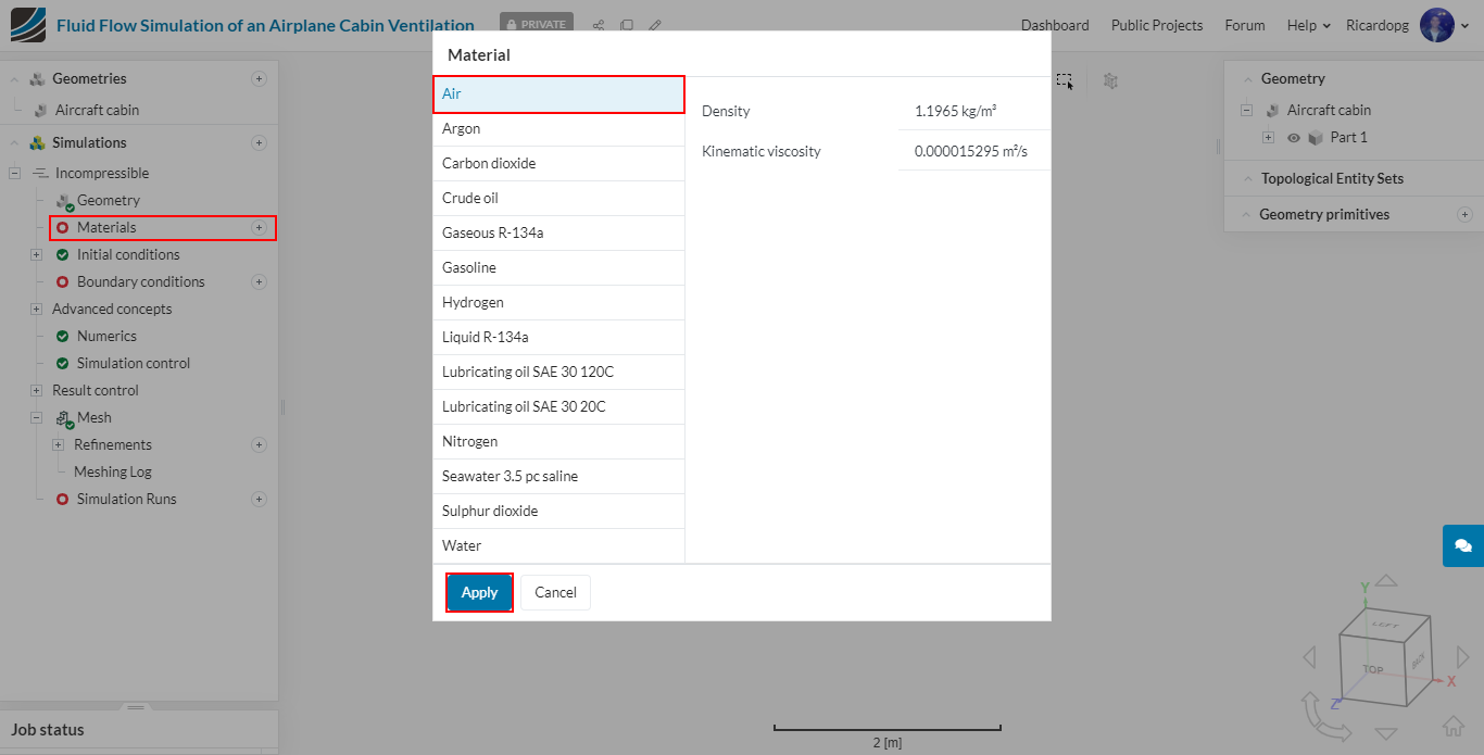
Air is automatically assigned to the flow region, so just click on the blue mark to save:
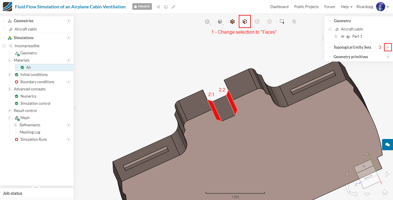
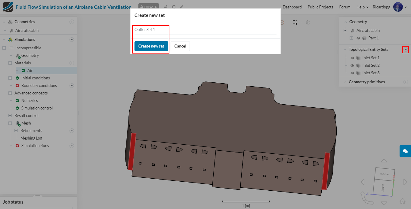
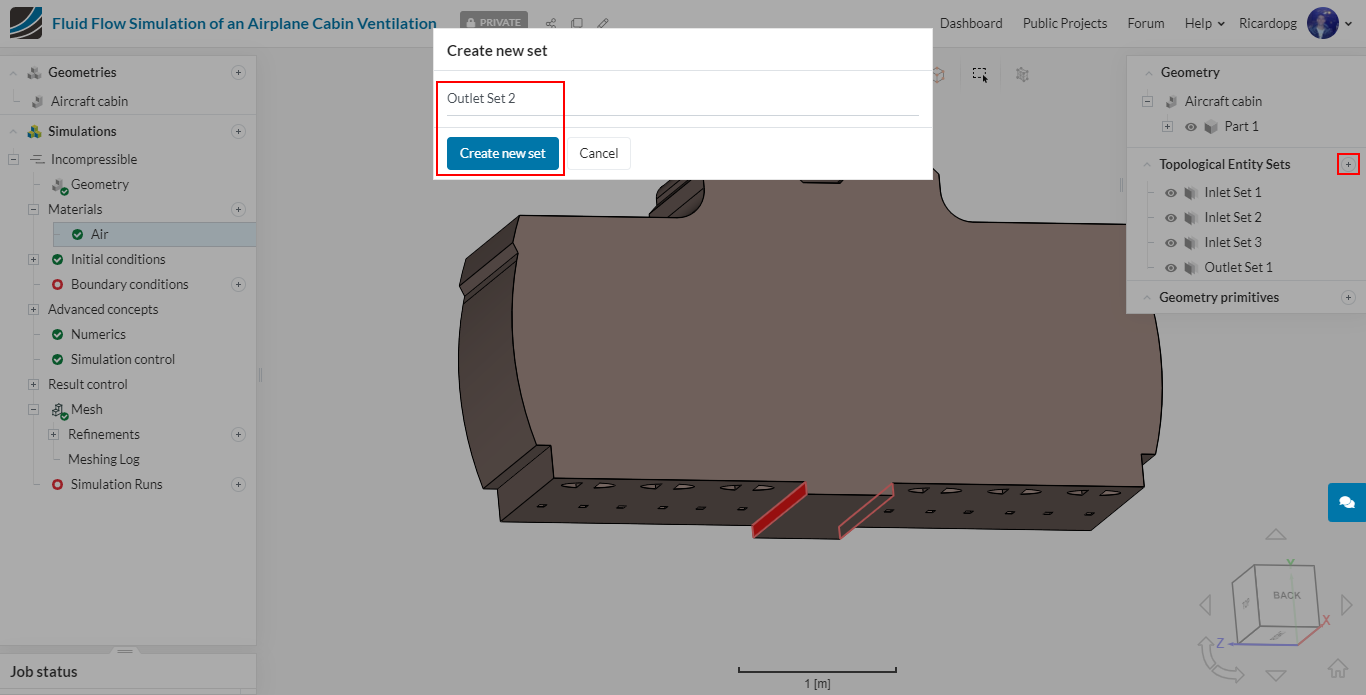
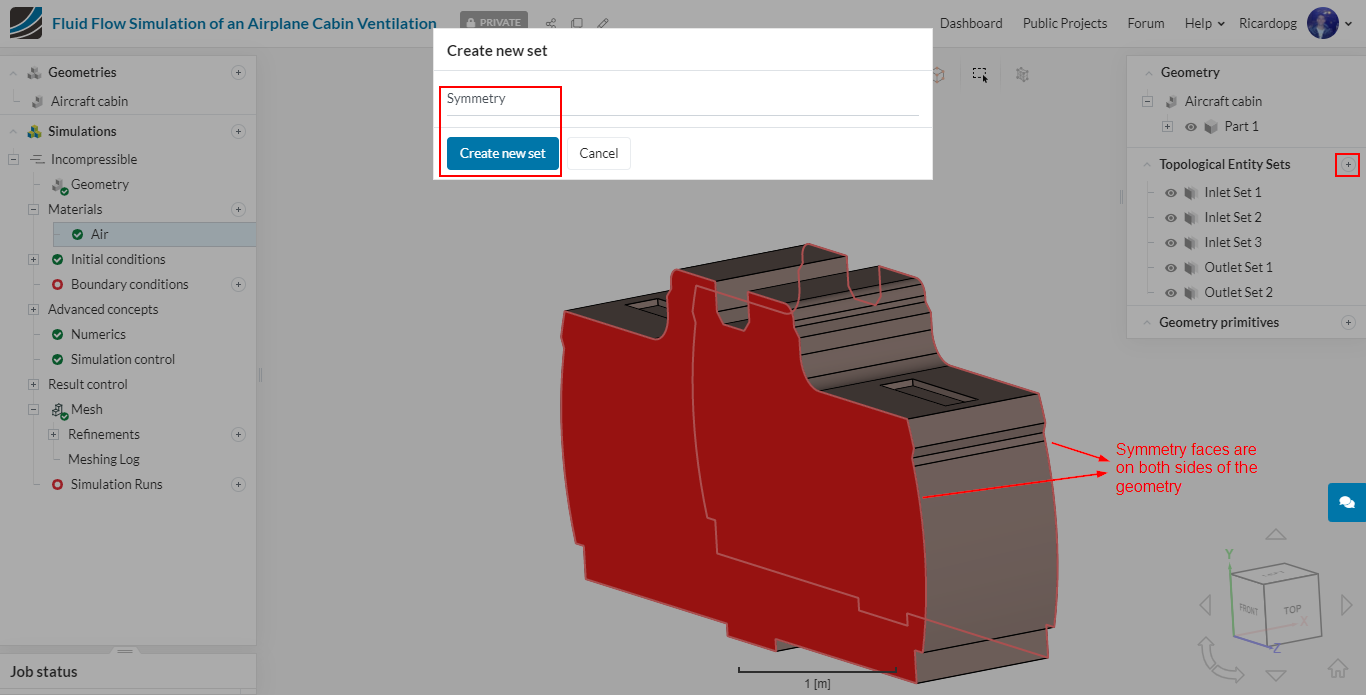
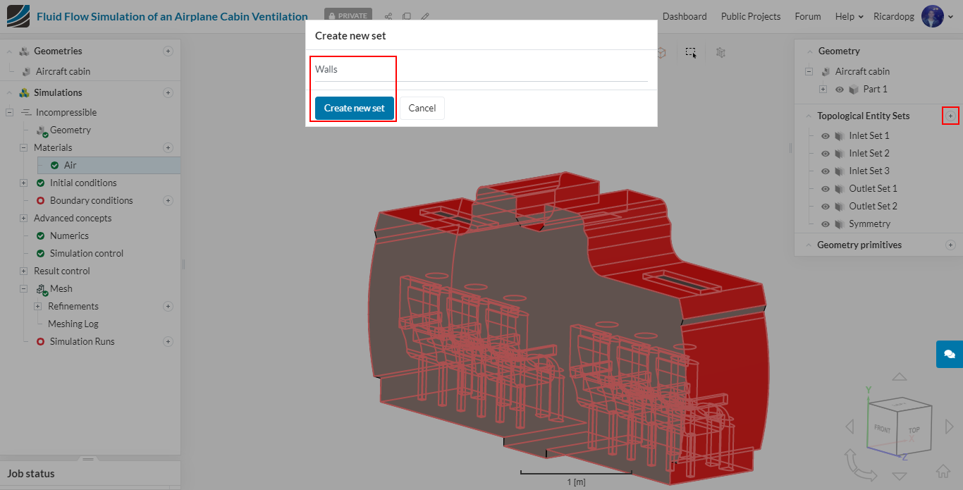
It’s time to create Topological Entity Sets. To create new topological entity sets, the following steps have to be followed:
- Select the face or faces that will be part of the newly created set;
- On the right-hand side of the screen, next to Topological Entity Sets , click on the + icon;
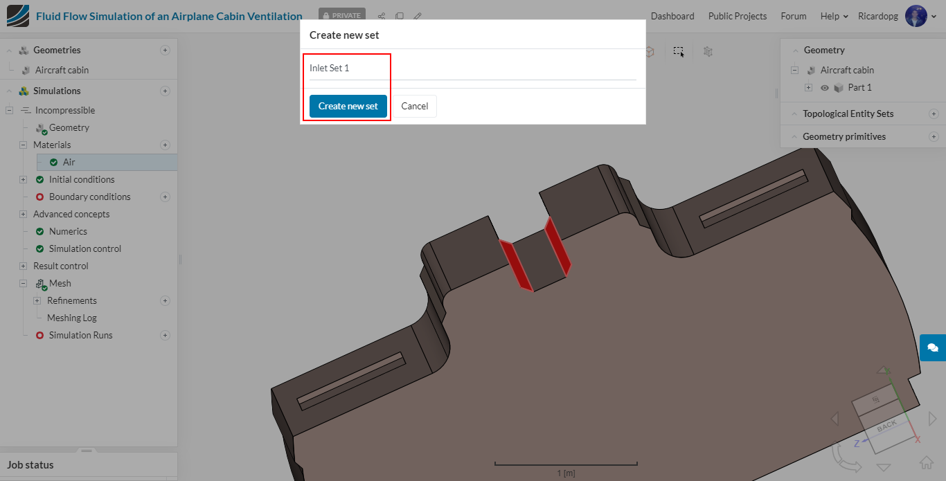
- Name the new entity set as you deem suitable.
This picture that was also posted in the beginning of this Step-by-Step will help us create the sets:
And here is a summary of the sets to be created:
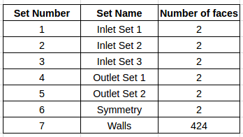
Inlet Set 1:
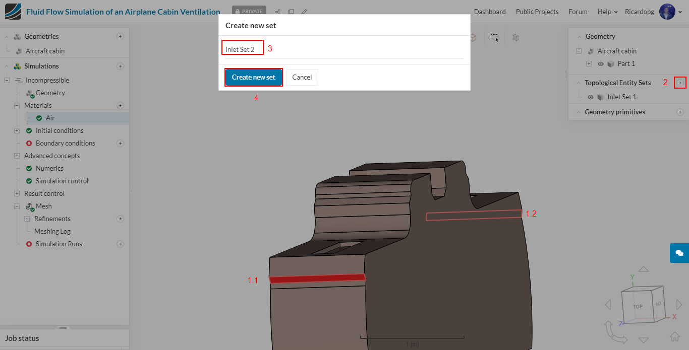
Inlet Set 2:
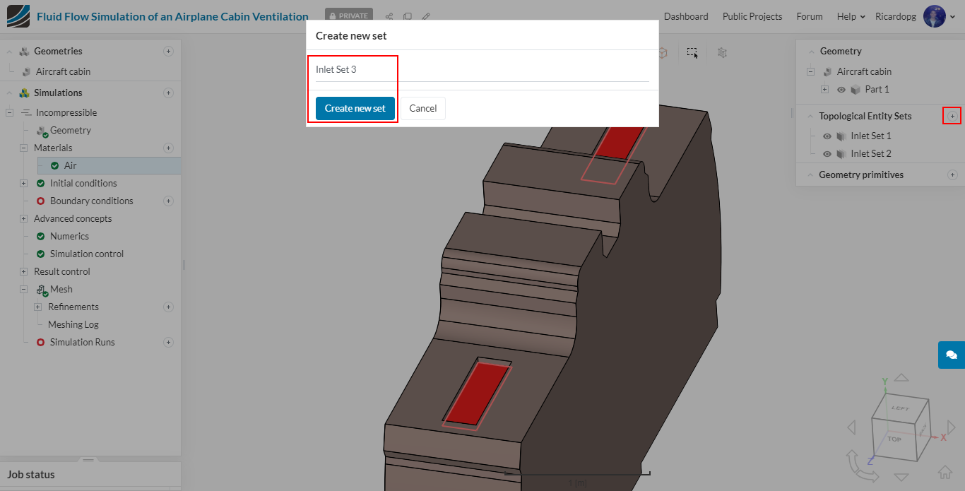
Inlet Set 3:
Outlet Set 1:
Outlet Set 2:
Symmetry:
Walls: in order to easily select all walls, please follow the steps below:
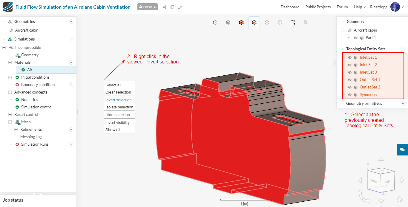
After doing this, all walls will be automatically selected:
Boundary conditions
The default Initial conditions will be used for these simulations. We will, therefore, jump straight to Boundary conditions. The boundary conditions (BC) define the flow variables at the boundary surfaces.
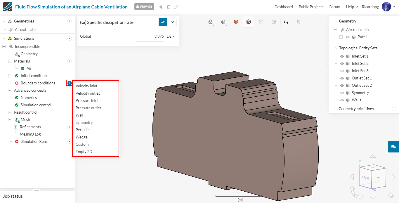
To assign a new boundary condition, click on the + icon and select the desired type.
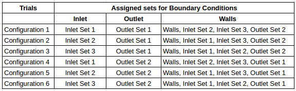
Configuration 1 will be covered in this step-by-step. When setting the inlet and outlet for different configurations, please refer to this table:
Boundary condition for the Inlet: it’s a velocity inlet boundary condition with a specified volumetric flow rate of 0.02975 m³/s.
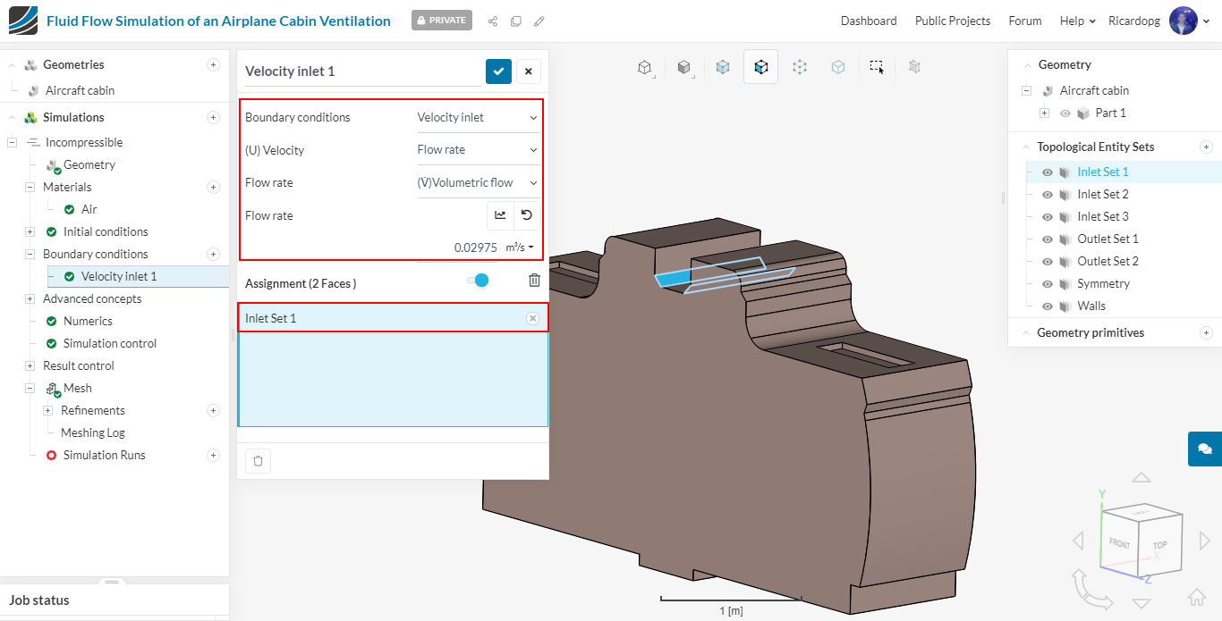
Important: for Configurations 3 and 6, please input an inlet volumetric flow rate of 0.07105 m³/s. These values were calculated so that an inlet velocity of 0.35 m/s is obtained.
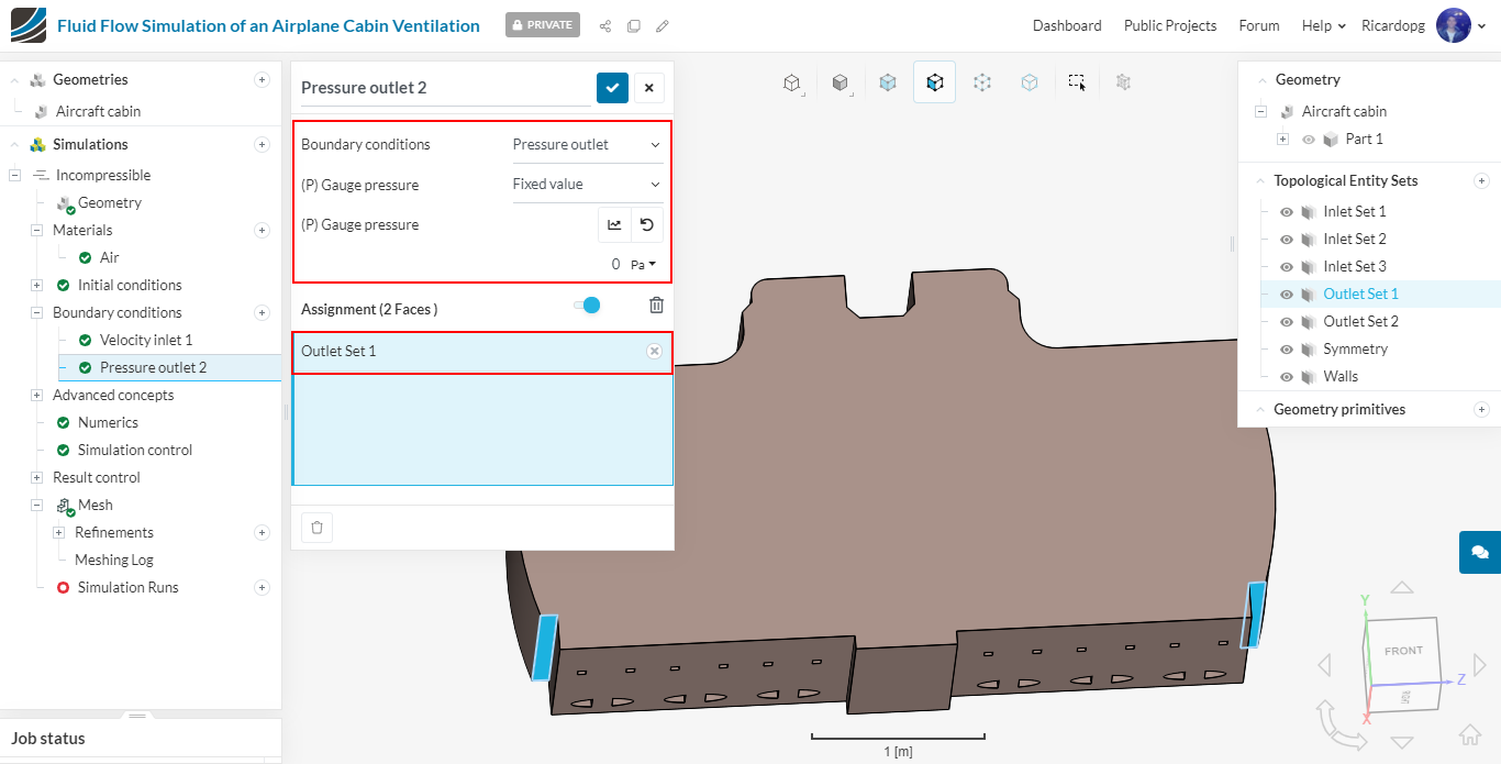
Boundary condition for the Outlet: it’s a basic Pressure outlet boundary condition with 0 Pa fixed value:
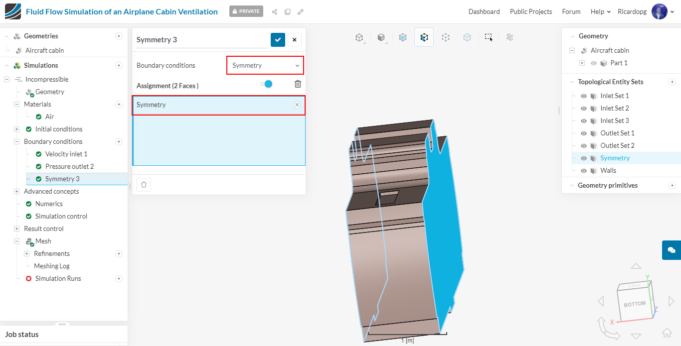
Boundary condition for the Symmetry topological entity set: Symmetry boundary condition:
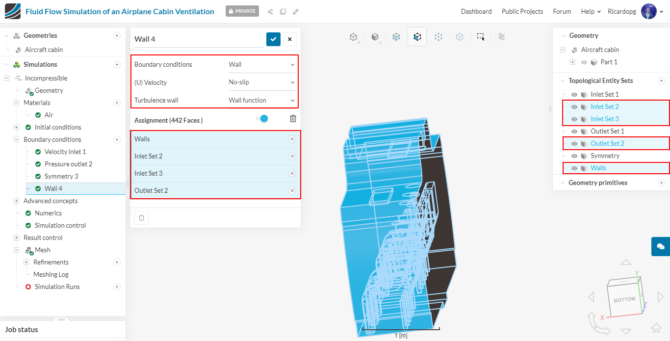
Walls: the remaining boundary definition is for the walls. One important thing to be noted is that this condition has to be assigned to all entities which are not defined the previous 3 conditions. Thus, it will vary from configuration to configuration.
For the Configuration 1, the following entity sets will be treated as walls: Walls, Inlet Set 2, Inlet Set 3 and Outlet Set 2:
Numerics
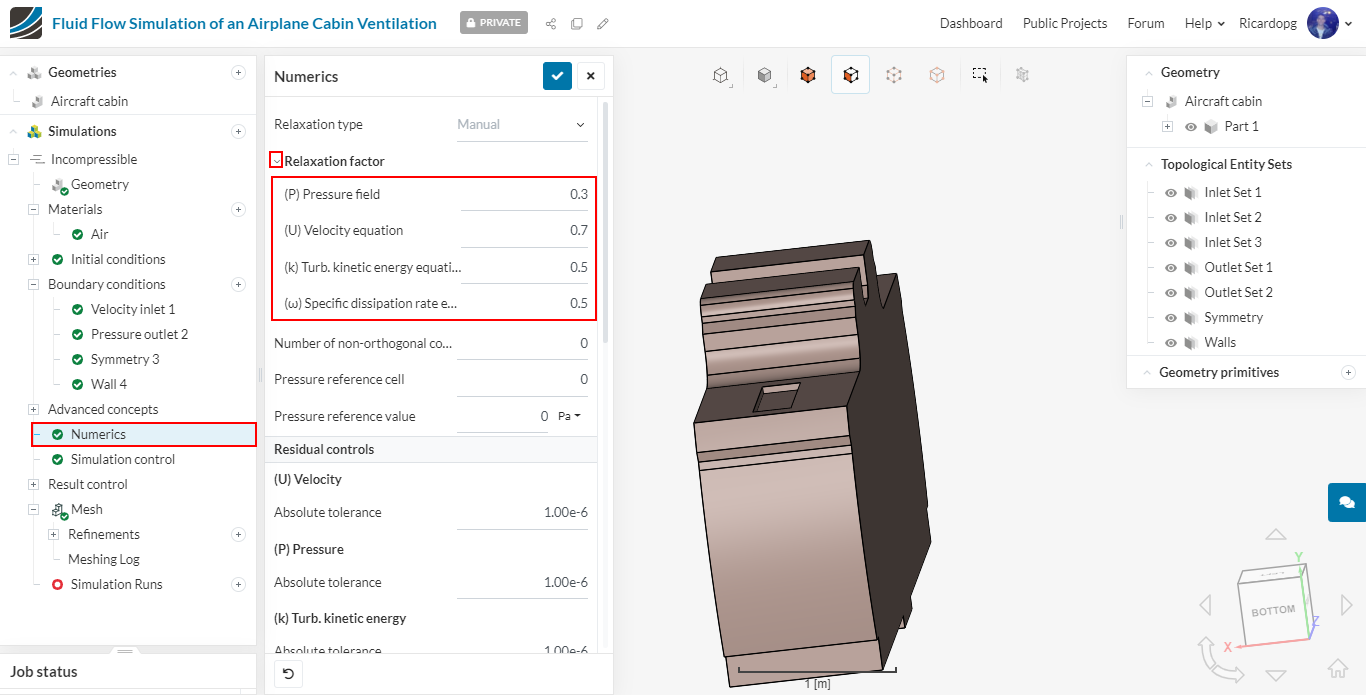
Please navigate to Numerics in the simulation tree. Set the Relaxation factors to the ones below. This enhances the solver to get the appropriate results:
- P : 0.3
- U : 0.7
- k : 0.5
- Omega : 0.5
Scrolling down through the numerics panel, find Solvers. Expand the ( P ) Pressure solver and set its Relative tolerance to 0.01.
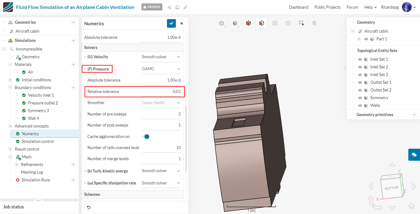
For the other solvers, make sure that Smooth solver has been selected. Change the Smoother to Sym-Gauss-Seidel:
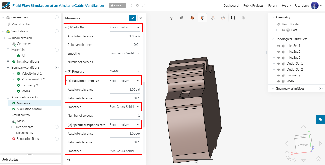
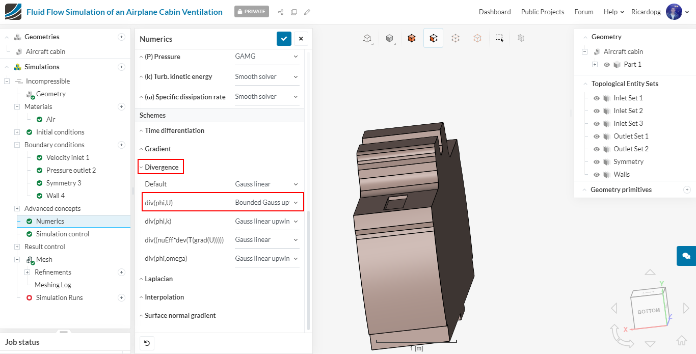
In Schemes, enlarge Divergence and select Bounded Gauss Upwind to div phi(phi,U).
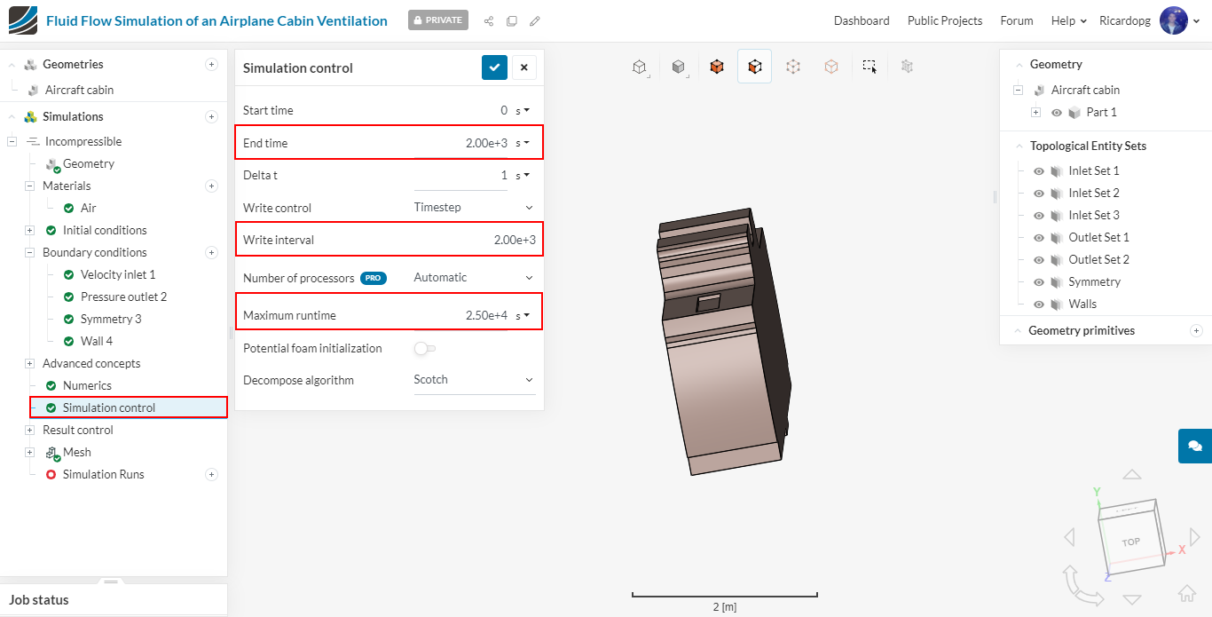
Simulation control
In Simulation control, change End time and Write interval to 2000 iterations. Also kindly adjust Maximum Runtime to 25000 seconds. You also don’t have to worry with the number of processors for the simulation run, as it is automatically optimized by SimScale:
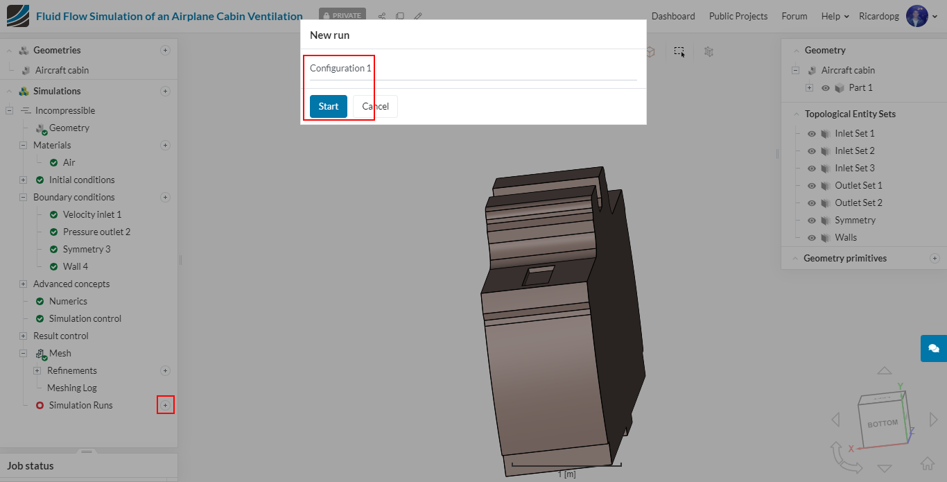
We are ready to run our simulation for the first configuration! So please head to Simulation Runs and Start it:
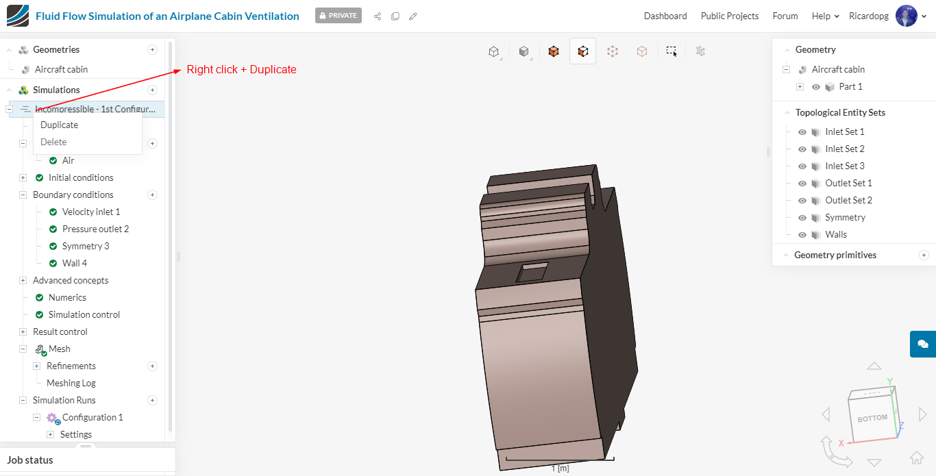
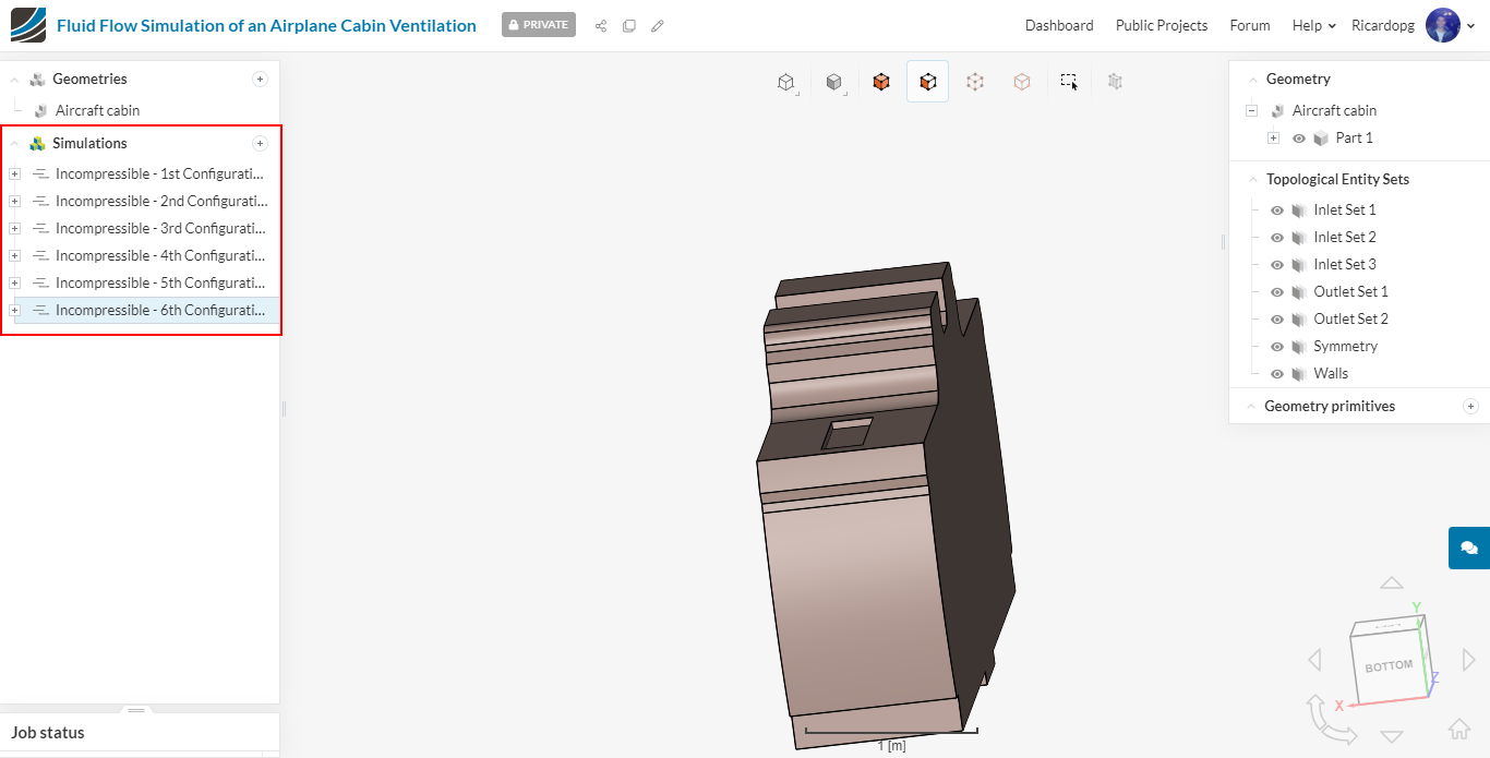
Now you can also create the other configurations and run them. You can run several jobs in parallel using SimScale, so there’s no need to wait for the first run to finish. To keep the project organized, you can Duplicate the first Incompressible setup and then adjust the boundary conditions:
Here is a table with the summary of the sets to be assigned to the boundary conditions. Please note that only the Symmetry boundary condition remains the same for all six configurations.
Post-processing
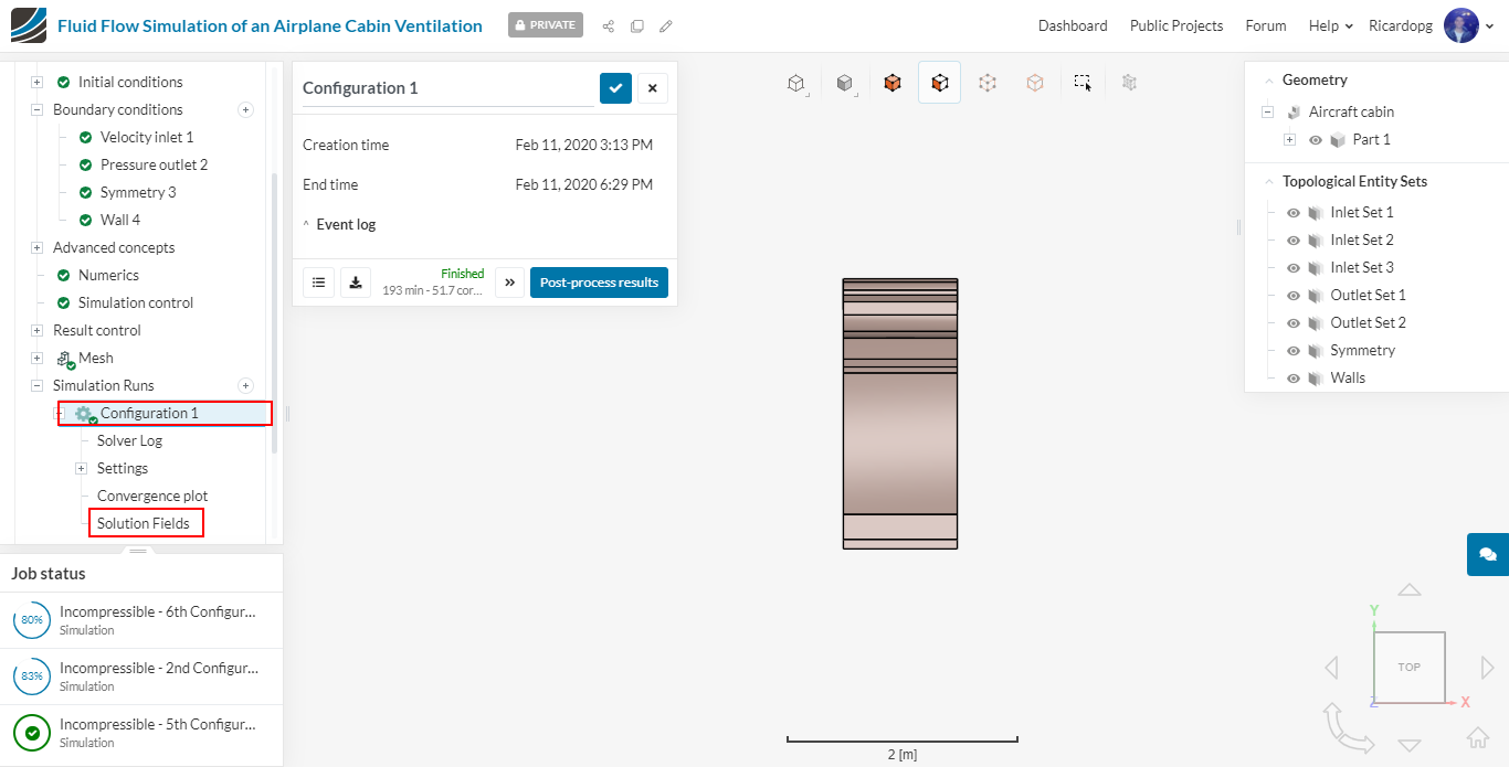
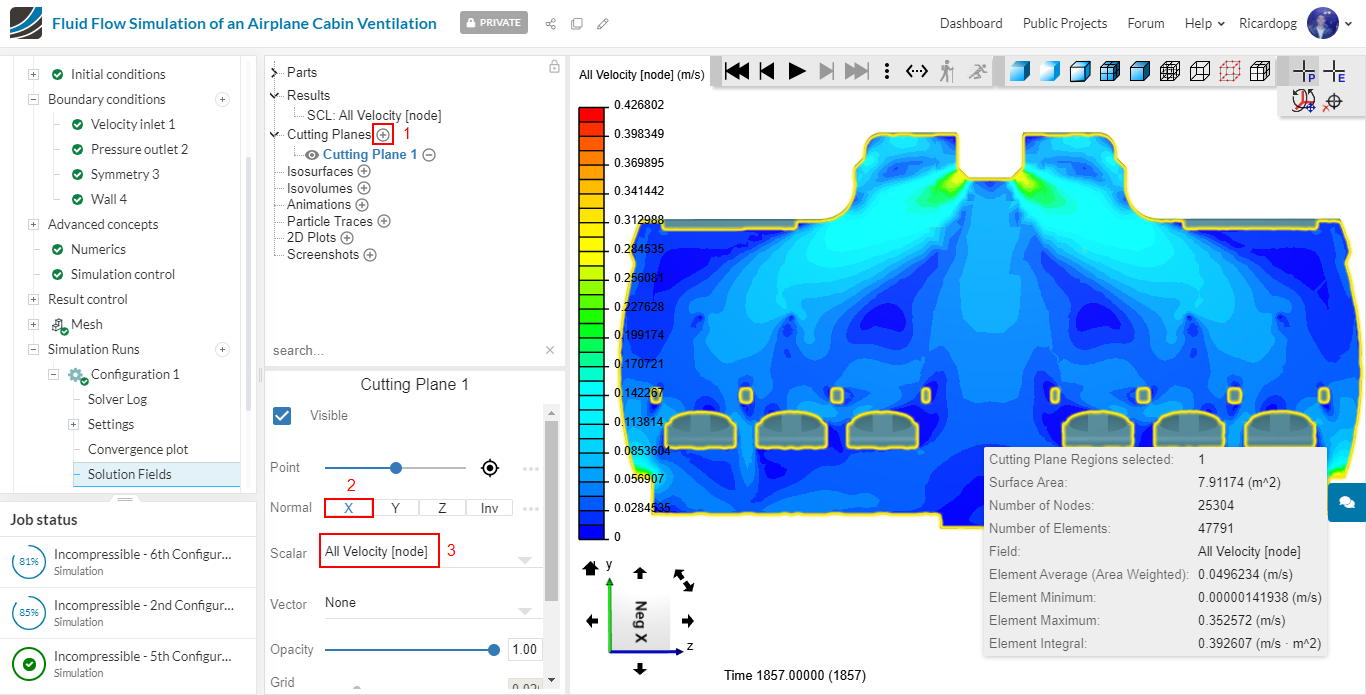
After the simulation run is finished, click on Solution Fields to go to the post-processing environment:
In the post-processing environment, there’s a panel towards the left-hand side of the screen with some filters and functions. Click on Cutting Planes to create a slice on the geometry. Select X to change the plane orientation.
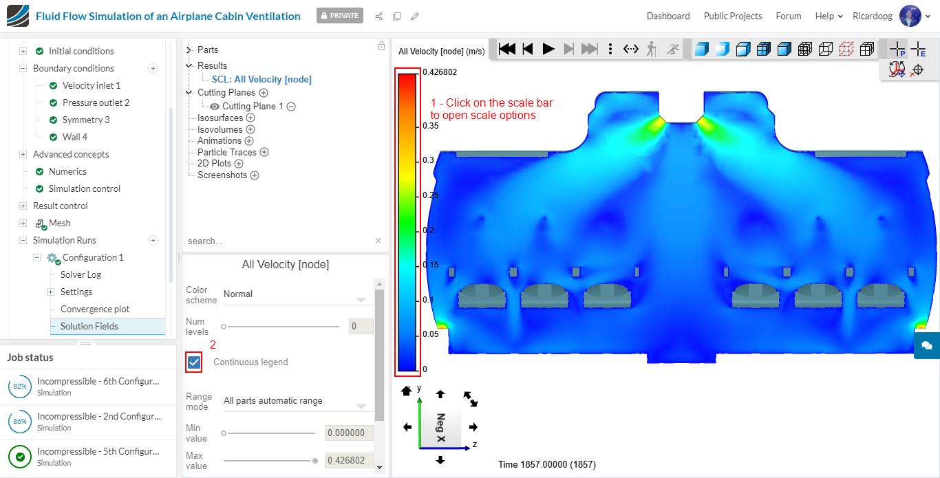
Now we will change the scale settings to make the transitions smooth. Click on the scale bar and select Continuous legend:
You can also plot velocity vectors on the cutting plane. To do so, click on the cutting plane and assign Velocity [node] to Vector:
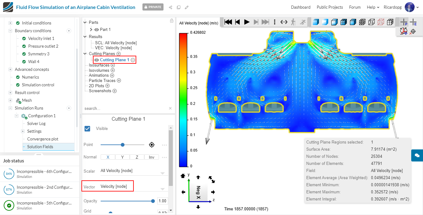
Several recirculation zones are easily spotted using this filter.
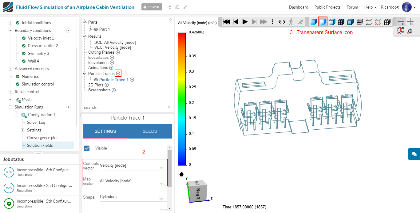
Other useful filter to be used is Particle traces. It generates streamlines which allow you to see what paths particles are making in the domain.
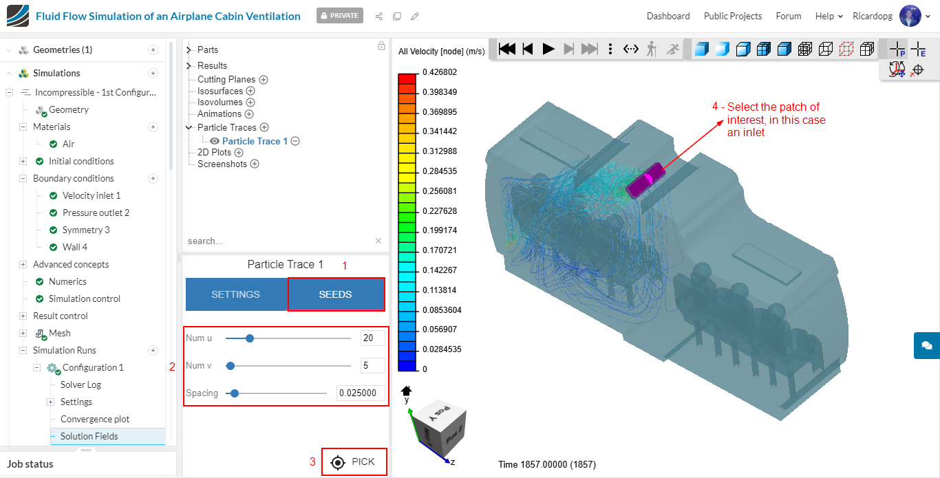
After creating a particle trace filter, change Compute vector to Velocity [node] and Map scalar to All Velocity [node]. Also change the surface representation to Transparent Surface by clicking on the highlighted icon shown below:
To add streamlines, click on SEEDS and then on PICK. Select a face of interest (usually inlet or outlet). The streamlines are highly customizable. It’s possible to change spacing, radius, number of lines, shape of lines, and map coloring.
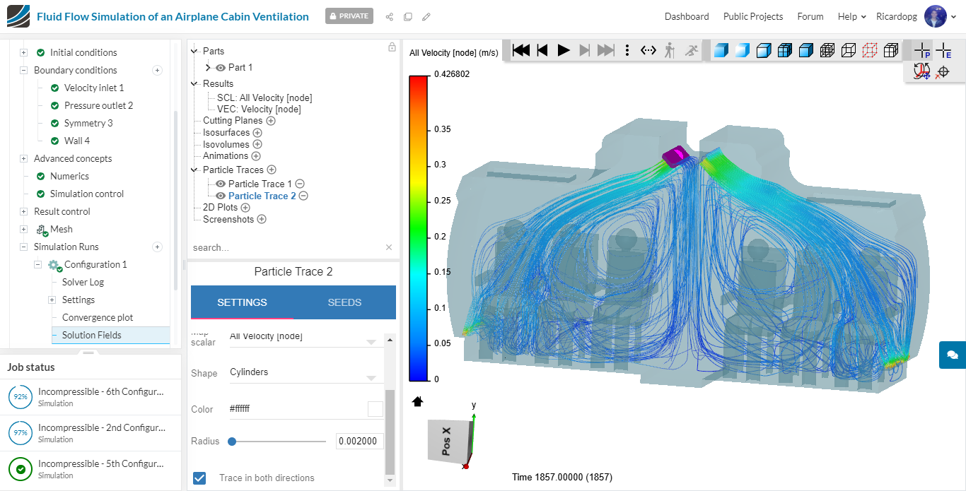
Create another particle trace, this time for the other inlet and have both of them displayed at the same time:
Similarly post-process the other configurations and compare them!