Ok i need to work through this bombshell of info … can i go back to the “Look my CFD has pretty colors” phase?
Lets give this a go:
Ill post one at a time so its not a 4 page long thing,
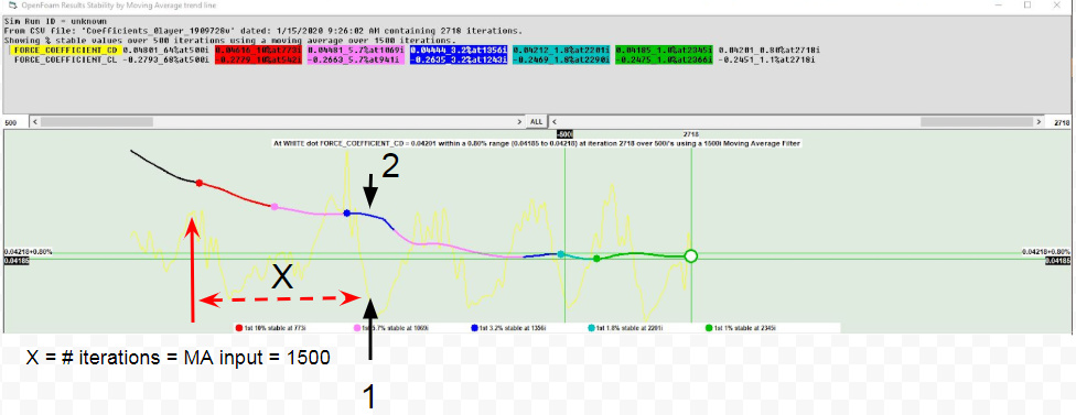
So in order to calculate the MA, we will take point 1 on the yellow data line and treat it like it is brand new, visualizing that there is nothing ahead of it on the graph as it hasnt been calculated yet.
The moving average is calculated by taking the sum of the raw yellow data values (red dashed line) for the previous 1500 iterations as set by our MA input.
Then this sum of values is then divided by the total number of iterations values recorded, which is 1500.
This produces the point 2 on the Moving Average Line, and the process continues for the next iteration
Yes, for each iteration, a 1500 point MA is calculated as you say but for iteration < 1500 I chose to calculate its MA by summing all the yellow values up to and including that iteration and divide by total number of iterations at that point (a fine point here but needs inclusions I guess)…
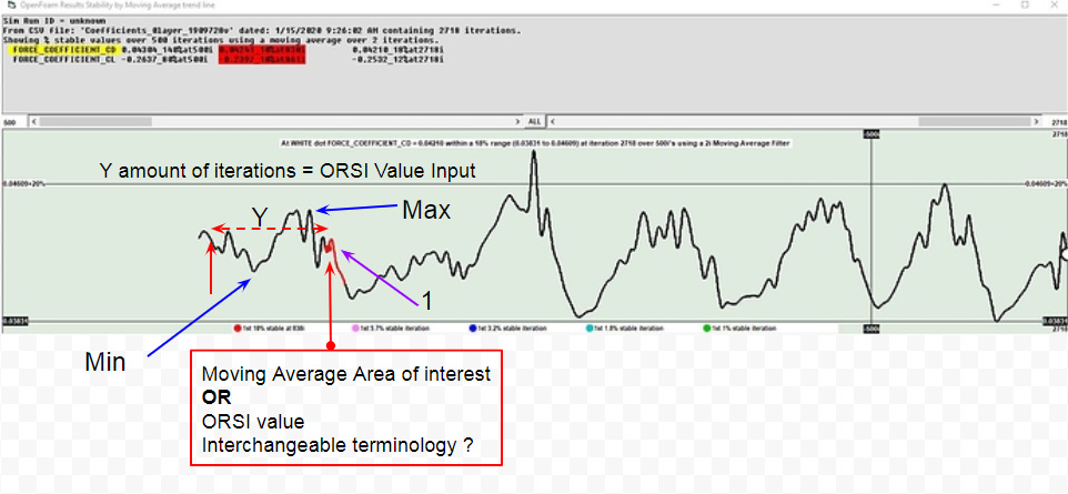
After the MA line is calculated we get the next graph which has an all black line
So almost the same procedure as before. At a point of interest on the black line MA graph, the ORSI% value is found by taking the Min and Max values within the predetermined # of iterations fro ORSI value, which is the dashed red line called Y. Then calculated as you said 100*(Max-Min)/ORSI
My question is does the output of this calculation produce point 1, the purple arrow? So it functions just as the last calculation did, where all data forward of point 1 is not yet existent and this is how it is made?
Point 1 is just an MA at the ‘IIteration of interest’ and IS the ORSI value… The ORSI % is the subject of the second Y window…
The fact that all data forward of Point 1 does not need to exist in order to calculate an ORSI value and an ORSI %, is the key to having the ability to use the ORSI % as a metric to being able to stop a simulation at the correct point, according to your own stability % preferences, in REAL time…
ahhh ok so the calculation is outputing the OSRI % or the divergence away from our point of interest ORSI value. This is why we see +X% and -X% of the ORSI value. Should have been apparent from the equation calculating min/max.
Ooops, sorry, I forgot, I chose to make ORSI % a magnitude item and took the absolute value formula as ABS(100*(Max-Min)/ORSI)…
There is still a small issue for a less realistic situation where stable parameters have the Max>0 and the Min <0… I chose to ignore that case for now until I figure out how to handle it…
Oh i see. nevertheless this is still much more accurate then i could have anticipated for my simulations. I have another sim running until 5000 and will be monitoring it when it reaches over 1000. I assume it will take until around 3000 like the rear wing did to reach 1%. Ill post the results when i get them
BTW I really appreciate you taking such a detailed look at ORSI by Moving Average… it is hard to do things like this on my own, without scrutiny… It is soo easy to make a coding or logic error
EDIT: It all started when Dylan said that he stops simulations when the results are 1% stable for the last 500 iterations, that sounded soooo easy
I have also made this guide in google docs for the other members of the AERO team so they can learn your programs as well. With your permission I will teach them your ways. Feel free to edit anything in the doc, i left it so you can change the contents
oh sorry, yes the file was taken from an incomplete csv file. it did work however when it wasnt complete, i just had to re click the yPlus_area. Maybe for the error i just happened to click when the line was not finished as shown in your picture above
I simplified the CAD geometry a little and then began layering it…
I decided that 5 layers was going to be too hard to achieve on this geometry for a 3.9 mm 1st layer and a 1.2 ER…
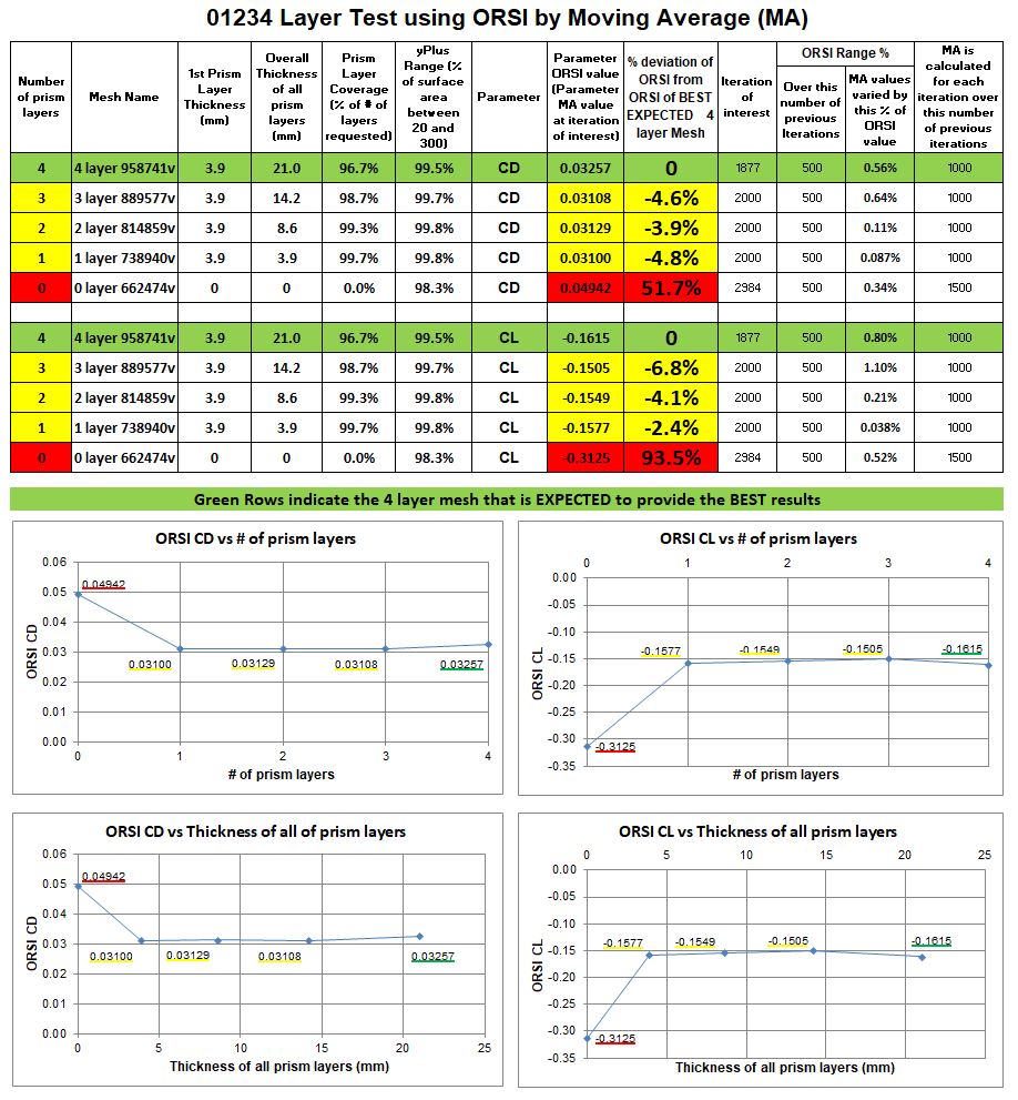
I did achieve 1 to 4 layers with 3.9mm 1st layer and 1.2ER and the ONLY change when I meshed each was in the Layering Refinement for each mesh… This ensured that the meshes were very similar with regard to everything but the number of layers and the total thickness of all prism cells…
Since the layer expansion ratio was a constant value of 1.2, the result was that the total thickness of the sum of the prism cell layers increased with each layer added… In doing this I believe I was investigating how important it is to encompass the near surface BL area using prism cells…
From 1 to 4 layers the total thickness of all prism layers increased from 3.9mm to 21mm…
Soooo, if the project holds up to scrutiny, my findings are that I am unable to determine any converging results relationship in using a larger number of prism layers or a larger Total thickness of the Prism cells…
The only conclusion I think I can make is that 1,2,3 or 4 layers are all equally expected to give better results than 0 layers (this assumes that prism cells indeed are needed for more accurate results, since the 0 layer mesh still had 98.3% of the surface area in the yPlus 20-300 range and the solvers do some no-slip wall calculations when there are 0 layers )…
Any comments out there (please scrutinize my project and conclusions thoroughly…)
I did make some edits… I did not see a save button…
Main changes were in where to extract the setup files from the zip file and what happens after you run the setup.exe… You might want to follow my instructions and get new screenshots…
Thanks for the feedback. Google docs is all online so no saving, it does that itself every few seconds. Thats why i like it, i can just sign into my google drive and access it from any computer, and with the link anyone else can view or edit. I will add any extra screenshots from the steps you put in.
Since I am a fan of the 1 layer approach, mainly due to its ability to play nice with my geometry, i have here shown your percent difference from the 4 layer run in numerical form.
Difference of 4 layer to 1 layer
Cd - 0.00156
Cl - 0.0039
To me this seems to be a very minuscule difference considering the level of accuracy you have already achieved. You already have all 4 test with Y+ values at 99% inside of the log-law region. So to me, what the increasing layers are testing is the area starting at the log-law region (around Y+=300) and seeing if the transition from turbulent boundary layer to normal velocity is effecting the Cl or Cd through the extra layers capturing these regions. It seems like it does to some extent, but as you said there is no direct correlation between the increase in layers and increase or decrease of measured Cl or CD.
Therefore, would this be proof that the HEX cells are capable of accurately capturing this transition data accurately enough that a 1 layer BL is justified?
I would also like to know how this test would go for a complex geometry such as mine. Would the much larger amount of turbulent areas create a positive correlation between # of prism layers and CL and CD?
I only ask this because the single wing test does have a turbulent section, but in a large geometry, the amount of turbulence in so many different areas could possibly help to make this test more definitive. However i think a 4 layer, 21mm boundary layer might cause some mesh problems haha.
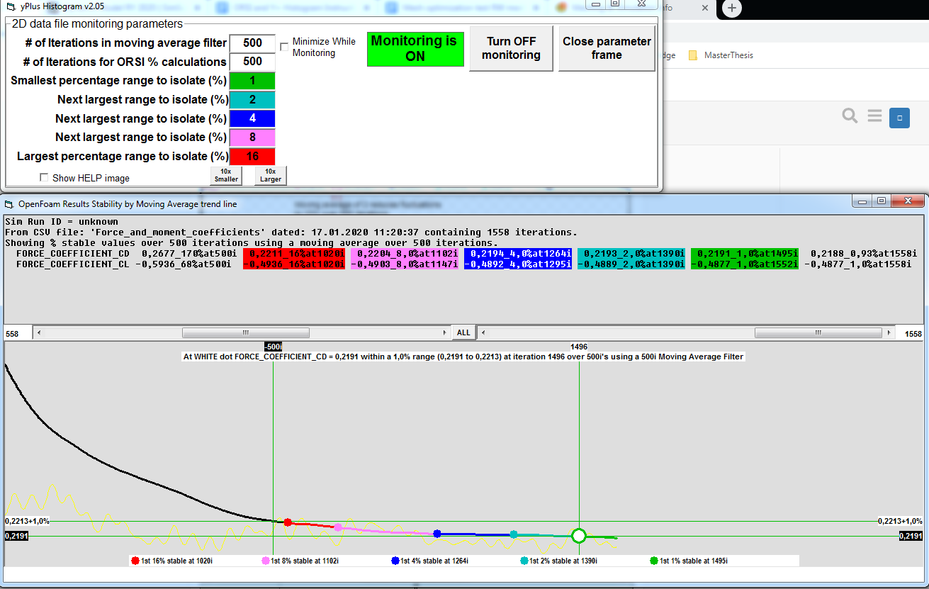
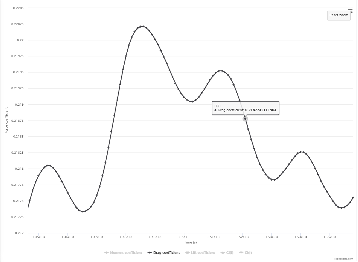
I also have the results from the half car sim. I unfortunately forgot to increase the maximum run time so it canceled around 1500 iterations. However it did achieve a 1% stability region so i know a 2000 iteration run will be ok
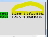
Then, all that is left (if you really want the best full set of data solution that matches ORSI) is to full re-run that sim run to end iteration of 1521 and voila, you have a final iteration full set of results at (or very close) to the ORSI CD 0.2188 value (And at that point I am pretty darn sure we are presenting the best guess of the solvers for that sim setup, at that ORSI % stability )