Hi everyone,
After doing some research, I complied a small document in order to understand why my simulations are not converging very well, and how the mesh quality effects this convergence ability. Mainly focused on Non-Orthogonality, I attempted to give some advice on how to treat solvers when mesh quality is not very optimal.
I would appreciate input from the Power Users: @Retsam @DaleKramer @Kai_himself @Ricardopg
The sources of information used:
Improving the quality of finite volume meshes through genetic optimization
OpenFOAM 6.3 Solution and algorithm control
Google Search
Error Analysis and Estimation for the Finite Volume Method with Applications to Fluid Flows by: Hrvoje Jasak
Videos
What is Mesh Non-Orthogonality
What is mesh Non-Orthogonality: The Over-Relaxation Approach
1. What is Non-Orthogonality?
Non-orthogonality measures the angle between two faces of the same cell. In a grid with only rectangular cells the value would be zero. Any deviation from this counts as non-orthogonal.
Example 1:
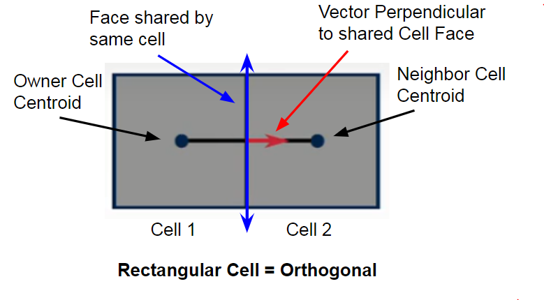
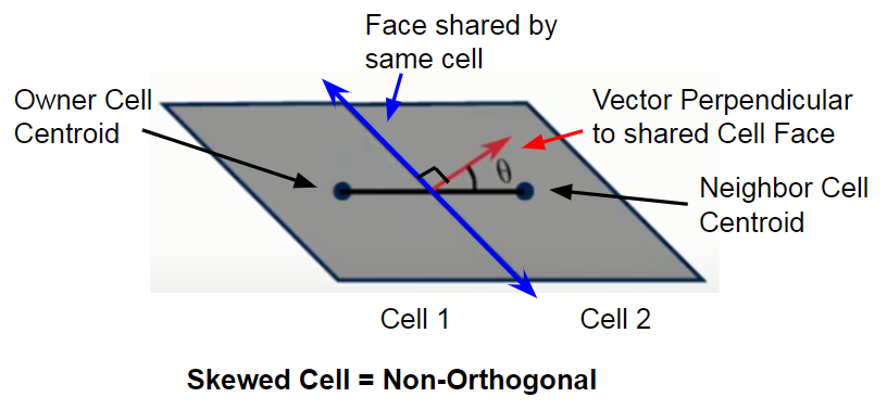
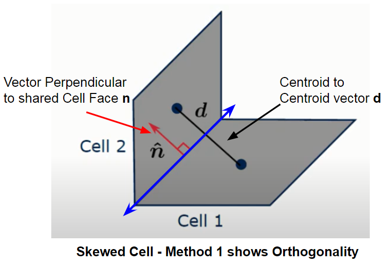
In Example 1, a vector perpendicular to the face shared by both cells creates an angle θ in relation to the vector connecting the cell centroids of the Owner (cell 1) and Neighbor (cell 2). This is the Non-Orthogonality angle. However, in example 2 we can see how this description would cause confusion.Two skewed cells in example 2 show that both the vector d connecting the centroids and the vector n perpendicular to the shared face, are parallel, which would result in an Orthogonal result. These cells however, are clearly not orthogonal to each other, which is why the code uses a second method to define Non-Orthogonality.
Example 2:
Non-orthogonality in method 2 is defined as the angle between the shared face vector n and the vector created from cell centroid 1 intersecting the midpoint of the shared face, given as vector c. This now allows for an accurate representation of Non-Orthogonality between these cells.
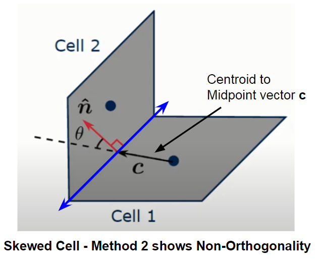
Before the simulation is run, every face on a cell is checked for Non-orthogonality by calculating vector d and vector c. This is defined as Face based Non-Orthogonality. The code then takes the largest non-orthogonal angle of all the faces in the cell and uses this as the final Non-orthogonality angle, defined as the Cell based Non-orthogonality.
2. Why is Non-Orthogonality important for CFD solvers?
In order to obtain accurate results, we need to consider the finite volume discretization of the diffusion term. I will attempt to avoid the complexities of this topic with an over- generalized, easy to understand explanation for why Non-Orthogonality is important for the solvers.
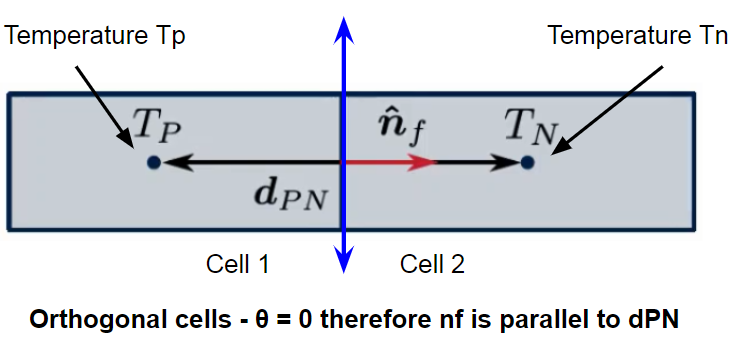
Let’s take the situation where we have two cells in our mesh with unknown values at the cell centroid shown as Tp and Tn. For this example the unknown value we want to find is Temperature, but this variable can also be calculated with velocity or pressure.Values important to complete these equation and find the temperature are the distance between the centroids and the magnitude of the vector perpendicular to the shared face nf. Since the cells are Orthogonal, nf is parallel to the vector between the centroids, dPN, making the solution very simple.
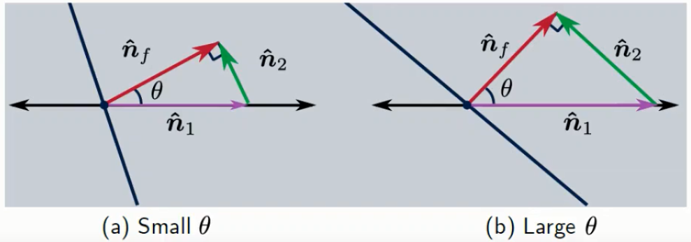
However, when the cells are Non-Orthogonal, as shown in the next picture, the shared face vector nf creates an angle θ relative to the centroid connection vector dPN. This requires the solver to break down the vector nf into two vector components. One component n1 is created so that it is parallel to the vector dPN while the other component n2 is used as the residual component in the vector decomposition.
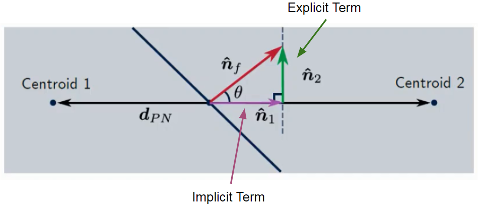
Vector n1 is defined as the Implicit term and is the Orthogonal component of the vector nf
- When n1 is large, it will increase the stability of the results and will help the convergence of the solution.
Vector n2 is defined as the Explicit term and is the Non-Orthogonal component of the vector nf
- The value of n2 is given based on the source term: the calculated values from the previous iteration. Since n2 is based on old data, it hinders the ability for the solver to move forward towards a convergent solution, and also increases instability in the results.
There are three ways that Non-orthogonal cells decompose the nf vector.
1. Minimum Correction (right triangle method)
This method creates a right triangle with vectors n1 and n2. At a low Non-Orthogonality angle θ, the magnitude of n2 is small so stability is not very affected. However, with this method, as θ increases, n2 becomes very large.
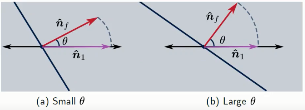
2. Orthogonal Correction (Rotation method)
This method simply projects the vector nf onto the centroid connecting line dPN where, vector n1 has the same magnitude as nf regardless of the Non-orthogonality angle θ.
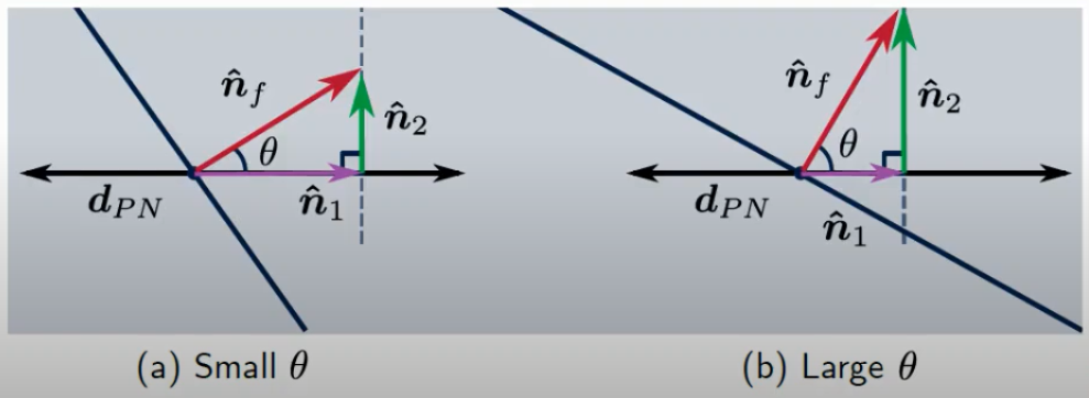
3. Over-Relaxation Method
In this method, a right triangle is created, with the right angle between nf and n2. As the angle θ increases both n1 and n2 simultaneously increase.
3. Which discretization method is the best?
The most common of these methods is the Over-relaxation method, due to the smaller amount of Non-Orthogonal corretor loops needed for a converged result as shown in the picture below. Since we now know that the value for the Explicit term n2 is taken from the previous iteration (source term), this value lags behind the solution for the Implicit term n1. Therefore, we are required to loop through iterations and update the n2 value, in order to get a converged solution for that Non-orthogonal cell.
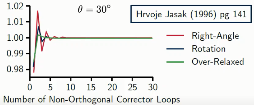
Even at higher Non-Orthogonality angles, the Over-relaxed method is able to deliver converged results while the Right angle and Rotation methods start to diverge.

Based on this information, we now know that when our mesh has some quantity of Non-Orthogonal cells, we must apply a certain number of Non-Orthogonal corrector loops in order to achieve a converged solution. From the following PPT, I was able to find a Tips and Tricks guide with the suggested number of loops based on the severity of Non-orthogonality in a mesh.
Non-orthogonality between 70 and 80
nNonOrthogonalCorrectors 4;
Non-orthogonality between 60 and 70
nNonOrthogonalCorrectors 2;
Non-orthogonality between 40 and 60
nNonOrthogonalCorrectors 1;
- What to do when Values of Non-Orthogonality over 70°
When the explicit term n2 is very large due to Non-Orthogonality, for example values over 70°, the solver must compensate for the errors of this variable and limit the value of n2 or discard it completely. The solver will then limit the explicit component in order to obtain a value smaller than the implicit component, which improves stability. This is done through the use of Under relaxation factors which are best described by the OpenFOAM user guide
Under-relaxation works by limiting the amount which a variable changes from one iteration to the next, either by modifying the solution matrix and source prior to solving for a field or by modifying the field directly. An under-relaxation factor
specifies the amount of under-relaxation, ranging from none at all for
and increasing in strength as
. The limiting case where
represents a solution which does not change at all with successive iterations. An optimum choice of
is one that is small enough to ensure stable computation but large enough to move the iterative process forward quickly; values of
As a summary:
- Non-orthogonality measures the angle between two faces of the same cell.
- Non-Orthogonality has a direct impact on mesh quality leading to potential errors in the simulation.
- The explicit term of the decomposed shared face vector is the cause of error but can be treated by updating the source term through introducing Non-Orthogonal corrector loops.
- The error causing explicit term can be further limited through imposing relaxation factors to force this source term to be smaller than the implicit term, leading to stability and convergence.
