Dear SimScalers,
in this weeks spotlight we will have a look at a CFD simulation of the Alfa Romeo P2 1930 by our PowerUser @pfernandez.
Introduction
The P2 was modified for season 1930 and won the Targa Florio that year, in the hands of Achille Varzi, who broke the average speed record for the race.^1

In this simulations, different configurations were considered:
- Without and with driver
- Static wheels and rotating wall on the tires
Geometry
Format: STEP
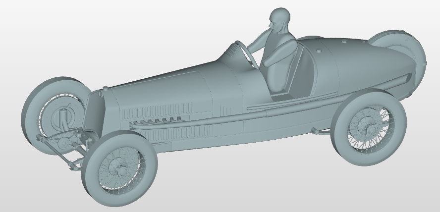
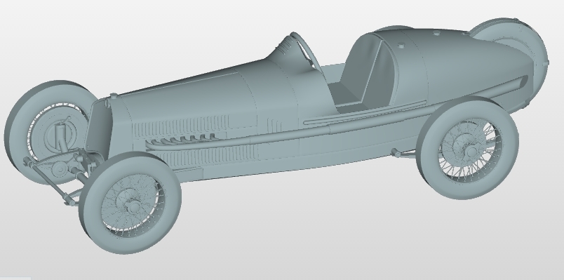
The 3D model of this italian race car is available at GrabCAD - Courtesy: Carco (GrabCAD). For the CFD simulations, a driver was also added. The mannequin used was also taken from GrabCAD - Courtesy: Emmanuel Mahay (GrabCAD).
Geometry with Driver
Geometry without Driver
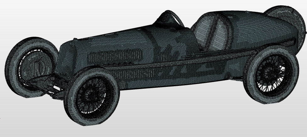
Meshing
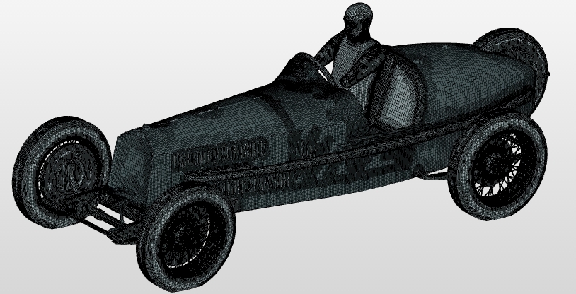
Type: Hex-dominant parametric (Snappy Hex Mesh)
Mesh with Driver
Mesh without Driver
The number of cells in the _BaseMeshBox can be chosen after setting the dimensions of the box. The size of the box can be based on different assumptions. In this case the virtual wind tunnel was defined to be about 10 times the length of the car and 5 times the width and height of the model with the car position towards the inlet and the floor intersecting the tires in order to simulate a contact patch.

This Google Sheet created by @pfernandez helped to get an estimation of the cell size and number of cells per refinement level.
Specify the material point to be within the fluid domain.
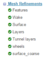
Mesh refinements
There are different kinds of refinements we can apply to our model in snappyHexMesh. Take a look at this tour by Engys for a comprehensive description of many of its features.
Features
The feature refinement identifies sharp edges on the geometry. In SimScale define the level to 0 because we just want to identify them so the meshing algorithm can take them into account. The cell size around the edges will be that of the surfaces close to it.
Wake
In order to capture the wake, we define a region with finer mesh around and behind the vehicle. For that we create a geometry primitive to define the volume we want to refine.

The refinement level was taken based on the spreadsheet calculations shared above.
Surfaces
The surface refinement for this geometry was split into three areas:
- Wheels: with a refinement level up to 7 (~2.6 mm) in order to capture the wheelspokes.
- Surface: general surface refinement up to level 6 (~5.2 mm) to capture most of the details of the vehicle.
- Surface coarse: with a refinement level up to 5 (~10.4 mm) for the large pannels of the bodywork.
Layers
In this simulation we left the default settings for layer addition on the faces of the vehicle and the tunnel floor.
The result is a mesh of ~11 million cells.
Simulation:
Type: Incompressible Fluid Flow Analysis
Turbulence model: K-omega SST
Materials: Air
Initial conditions
- Pressure: Leave the reference pressure as 0 \frac{m^2}{s^2} \rightarrow Kinematic Pressure
- Velocity: 40 \frac{m}{s} (144 \frac{km}{h}) in the x-direction.
- Turbulence properties: use cfd-online’s calculator to define the parameters for k and omega:
- k: 0.06.
- omega: 390.
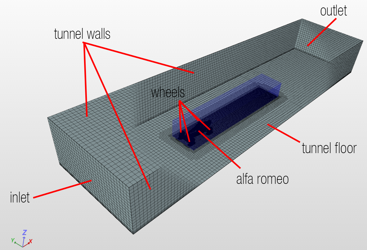
Boundary conditions
Six different types of boundary conditions were used for this simulation:
- inlet: velocity inlet of 40 \frac{m}{s} in the x-direction.
- outlet: pressure outlet with a reference kinematic pressure of 0 \frac{m^2}{s^2}.
- tunnel walls: slip wall boundary condition.
- tunnel floor: moving wall boundary condition of 40 \frac{m^2}{s^2} in the x-direction.
- alfa romeo: no-slip wall boundary condition.
- wheels: rotating wall boundary condition.
- use the CAD software to determine the axis of rotation of each wheel.
- use the wheel radius to determine the angular speed (52.359 \frac{rad}{s}) of the wheel.
Numerics
The residuals control were modified and the absolute tolerance was set to:
- 0.001 for pressure.
- 0.0001 for velocity, turbulent kinetic energy, and omega.
Simulation control
The end time was set to 3000 iterations which should be enough to reach an asymptotic value in terms of drag.
Result control
In this section SimScale can calculate the force and moment coefficients, amongst other results. To obtain the drag and lift coefficients we have to define the drag and lift directions, the freestream velocity, and the reference area.
Results & Conclusion:
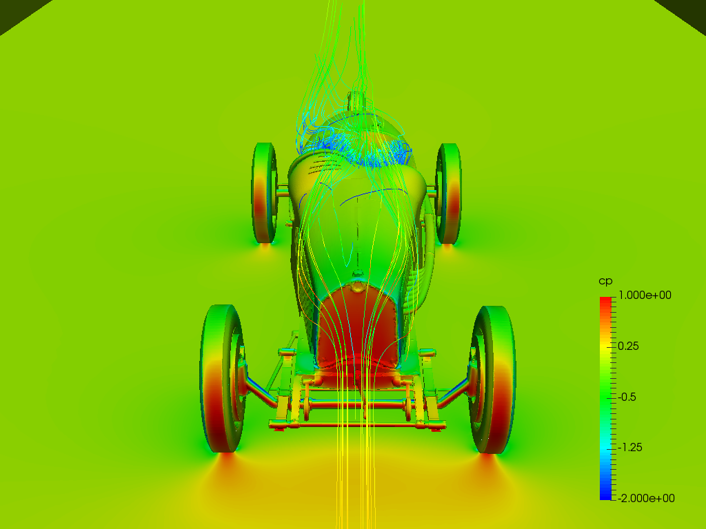
Drag
The following is an accumulated drag plot. The functionality was introduced in OpenFOAM 2.2.0 (see this controlDict as an example), and can tell us which areas of the car build up drag.
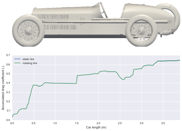
It is readily apparent that the blunt front bodywork of this racecar is responsible for nearly half the drag while the streamlined rear-end of the car adds very little.
Downforce
This early models have no aerodynamic devices so she should not generate any significant amount of downforce as the very low coefficient shows in the following plot.
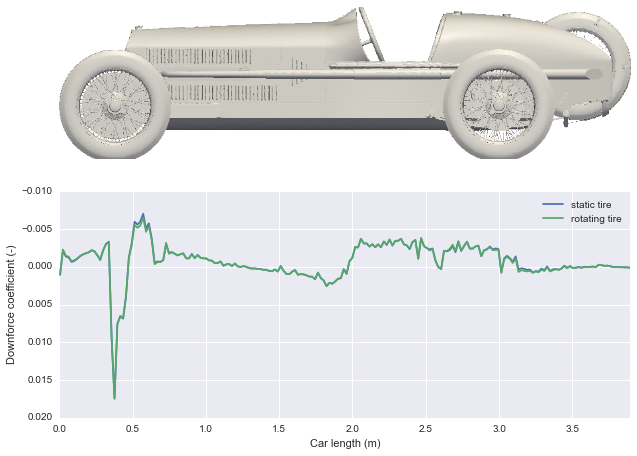
The inclined front along with the pressure build-up generate some downforce at the front wheel. The rest of the car is rather neutral but for the cabin which contributes some sustained lift.
Comparison
There seems to be little difference between a static wheel simulation and imposing a rotating wall boundary condition on the tires; but though little, there is.
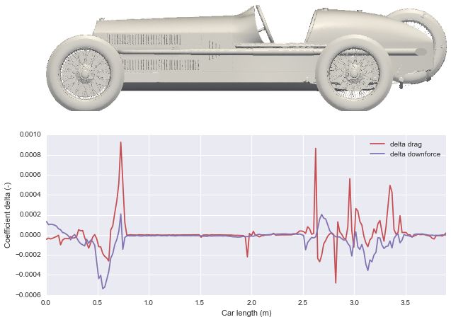
The results show static minus rotating.
Following the red line (delta drag), we can see that a rotating wheel build less drag at the back of the tire while the magenta line (delta downforce) suggests that a rotating wheel generate more lift at the front and more downforce at the back.
Driver
Now, what if we include the driver?
As the Alfa Romeo P2 is an open two-seater, the influence of the driver cannot be neglected. These are the results.
         +----------+--------+
         | Baseline | Driver |
+--------+----------+--------+
| Cd     |   0.651  |  0.634 |
+--------+----------+--------+
| Cd x A |   0.680  |  0.701 |
+--------+----------+--------+
If we only look at the drag coefficient we will stumble ourselves upon a surprising result; the drag coefficient without driver is larger? Everybody would expect otherwise.
Drag = 0.5 * rho * Cd * A * U**2
As we can see from the definition of drag, when we look at the Cd alone, we are not taking the reference area into account; and with a driver, the latter increases. So, we add the concept of drag area Cd * A which will allow us to compare results from different sources in a more equitable manner.
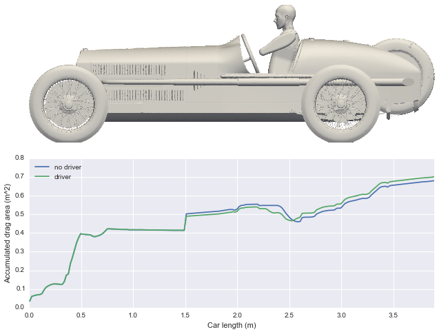
The plot shows that the effect of the driver is appreciable from the start of the cabin interior at 1.5 m as with the driver more pressure builds-up at the firewall.
Resources:
SimScale project:
To look at the simulation setup, please have a look at the project from @pfernandez :
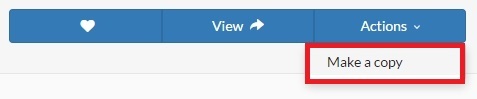
To copy this project into your workspace, simply follow the instruction given in the picture below.
\underline{\textbf{Visit our SimWiki by clicking on the picture}}