Hello everyone
I have a special topic that I wish to fully understand with your help. I have done some research however I have not found any conclusive results or articles that accurately describe the condition.The original thread that sparked this investigation is given here:
Starting on Pg 2 with the main description on Pg 4
The topic is:
The Center of Pressure (CoP) is used to help define the sum of all aerodynamic forces and moments about a singular point for a given system (in our case the entire race car). The common theory is that this point can give us an accurate description of the forces acting on the car when based from a certain origin point, usually the Center of Gravity (CoG). With this information, we can calculate the distance of the CoP to the CoG, which results in an understanding of the expected stability of the car.
According to the link and discussion above, this description of the CoP is an incomplete picture of the actual forces acting on the car. This is best said through quotes from the thread.
“The distributed air pressure forces of aerodynamics DO NOT have a "centre of pressure".
The resultant of the pressure forces is best described with a "force screw" (aka a "wrench"). This "dual vector" quantity acts along a "line of action", and NOT at any specific point, or "centre".”
To my understanding, the Aerodynamic forces are acting along a “line of action” (LoA), which is similar to a roll center, and is constantly changing based on the dynamic motion of the car.
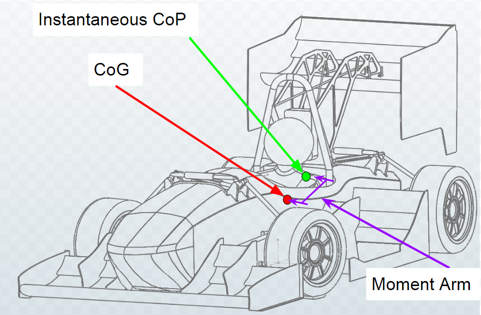
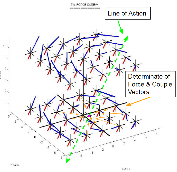
The original CoP theory is shown in the picture below, the Instantaneous CoP would be measured using the Forces and Moments result control in Simscale with the origin point at the CoG position. The value of the CoP is the result of a moment calculated from the CoG origin point, which will tell us the distance and force acting upon the CoG due to the summation of all aerodynamic devices. While this is useful in telling us overall stability, it does not give us information on the forces at the locations that really matter, which is directly at the contact patches of the tires.
Now going back to the topic of resultant pressure forces being described as a force screw. The force screw theory is described best by quoting the thread
“Consider a rectangular coordinate system with its origin fixed to some point on our car (could be the CG, but doesn’t really matter). X is forward, Y to the left, and Z upward. The car has been through the wind tunnel and we get the following "aero forces and moments", measured at the origin, for some wind speed and car orientation. (I’ll use "couples", labelled with Ts, because in the long run it makes more sense.)
Forces … Couples…
================================
Fx(0) = -300N, … Tx(0) = +600Nm.
Fy(0) = +400N, … Ty(0) = +800Nm.
Fz(0) = -1,200N, … Tz(0) = +2,400Nm.
We vectorially sum the forces to get a resultant force vector Fr(0) that points mostly downward, but also slightly backward and to the left. The magnitude of this resultant force is 1,300N (exactly!). Likewise, we sum the couples and get a resultant couple vector Tr(0) of 2,600Nm, which points mainly upward and slightly forward and to the left (using "RH screw rule").
We now draw the "arrow pairs", or vector duals Fr( P) + Tr( P), at Z=0 and Z=10. Then on an X-Y grid from -6 to 6 in steps of 3. Forces are red, couples blue, with their tails on the crosshairs, which represent the various points P. The couple vector at the origin Tr(0) is barely visible, hiding behind the Z-axis.
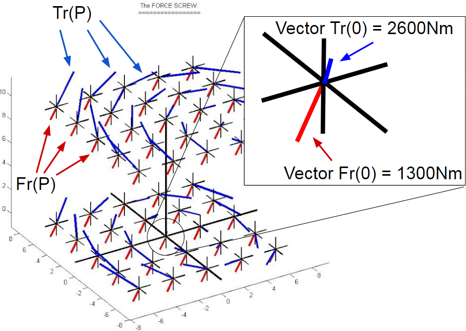
Fr(0) + Tr(0) is one way of specifying the "dual vector quantity" that fully describes the aero forces. So we draw some kind of 3-D picture of this with the two resultant vectors shown as arrows, with lengths proportional to some scale, and their tails at the origin.
But we also know that we can "calculate forces and moments" at any point. The origin was arbitrarily chosen, and is not special in any way. So it is time for some research. We start calculating new Frs and Trs at a whole lot of other points P.
The force Frs are simply moved to P unchanged (see note below). But new couple Trs must be calculated. The equations required are similar to Moop’s above, but with opposite signs (going in opposite direction?), and we have to include the original couples.
========================
Tx ( P )= Tx(0) + (-FzPy + FyPz)
Ty ( P )= Ty(0) + (+FzPx - FxPz)
Tz( P ) = Tz(0) + (+FxPy - FyPx)
=========================
Example 1. Point P(x,y,z) = (1,0,0)
Tx( P) = 6 + (120 + 40) = +6Nm.
Ty( P) = 8 + (-121 + 30) = -4Nm.
Tz( P) = 24 + (30 - 41) = +20Nm.
Example 2. Point P(x,y,z) = (10,10,10)
Tx( P) = 6 + (120 + 40) = +166Nm.
Ty( P) = 8 + (-120 - 30) = -142Nm.
Tz( P) = 24 + (-30 - 40) = -46Nm.
Technical notes. In the above, we are adding equal and opposite copies Fr( P) + -Fr( P), of the original resultant force Fr(0), at each point P. We can do this because together they sum to zero, so we are adding nothing. Fr( P) becomes the "moved" Fr(0), while the original Fr(0) + -Fr( P) becomes a new couple dTr( P) to be added to Tr(0).
Also forces are "sliding vectors" (they can slide anywhere along their LoA) and couples are "free vectors" (can go anywhere), but we put both Fr( P) and Tr( P) at P, to show that these are the "forces and moments calculated at P".
Importantly, we only need one of these "vector duals" to give a complete specification of the force system. However, we calculate lots of them to get a better view of the big picture.
This video accurately describes this process through solving determinants and cross products.

Basically I understand this as - when we select our forces and moments about a point (as said above this can be the CoG but not necessary), the resultant force and moment given about this point “P” is not along the line of action. The origin in this Force screw Fr(0) and Tr(0) picture above is also not along the line of action. To find this line of action, more is described below:
The maelstrom of swirling couple vectors clearly show a "helicoidal field" with a calm central axis. This axis is parallel to all the force vectors, and passes a short distance in front of and to the right of the origin. The further away from this axis, the more furiously the couple vectors swirl, like a tornado with wind speeds that increase without limit away from the core.
Looking closer, we see that this particular force screw has a left-hand thread. This was actually quite obvious from the beginning, because the force and couple vectors at the origin were pointing in approximately opposite directions.
At the central axis the couple vector is at its minimum magnitude, and is collinear with the force vector. Away from the axis the couple vectors always have this same component in the direction of the axis, but they gain increasingly large circumferential components at increasing radii. The circumferential component’s magnitude is simply |Fr| x radius.
All the above suggests that one way to specify any particular force screw is by giving four numbers to locate its central axis, together with two numbers for its force and couple magnitudes (with suitable definition of which is the +ve direction, etc.). So six numbers in all, with the two magnitudes being invariant to the chosen reference frame. Or we can use Plucker’s coordinates, but that is another story…
Interestingly, we see that any force system, no matter how complicated (eg. composed of a squillion little air pressure forces), can always be reduced to nothing more than the application of a screwdriver. Just a push and a twist along some axis. Or a wrench = "~n. a forceful twist or pull".
But, perhaps even more interestingly, if we had to build a structure to resist this "force system", then the most sensible place to put it is in "the eye of the storm". Here the forces (well, really only the couples) are at their smallest. If we put the structure far off to the side of the axis, then there are huge "bending moments" that must be resisted. This reason alone should be enough to encourage engineers to "always find the central axis".
Finally, there is a direct one-step method of finding the location of the screw axis, when given the force and couple vectors at a single point. The direction of the axis is parallel to the resultant force vector Fr, and the axis' radial distance away from the point is found by considering the circumferential couple component, as briefly described four paragraphs up.
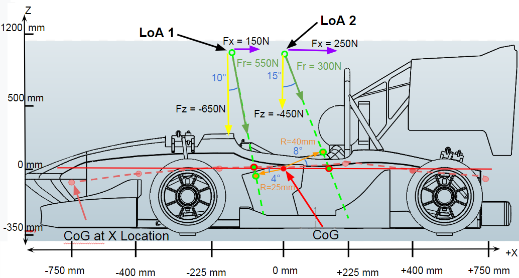
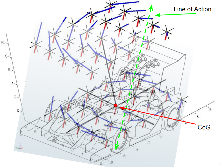
Relating this to our FSAE car, If we select the origin point for the forces and moments calculation, the Force Screw would look something like the picture below. The selection of the CoG is irrelevant as the Line of action can be calculated from any point selected. The way to find the line of action is described above as multiplying the force component (Fr)by the Radius.
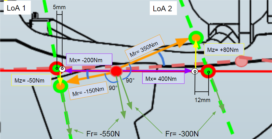
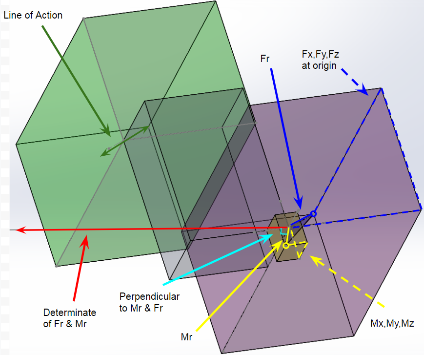
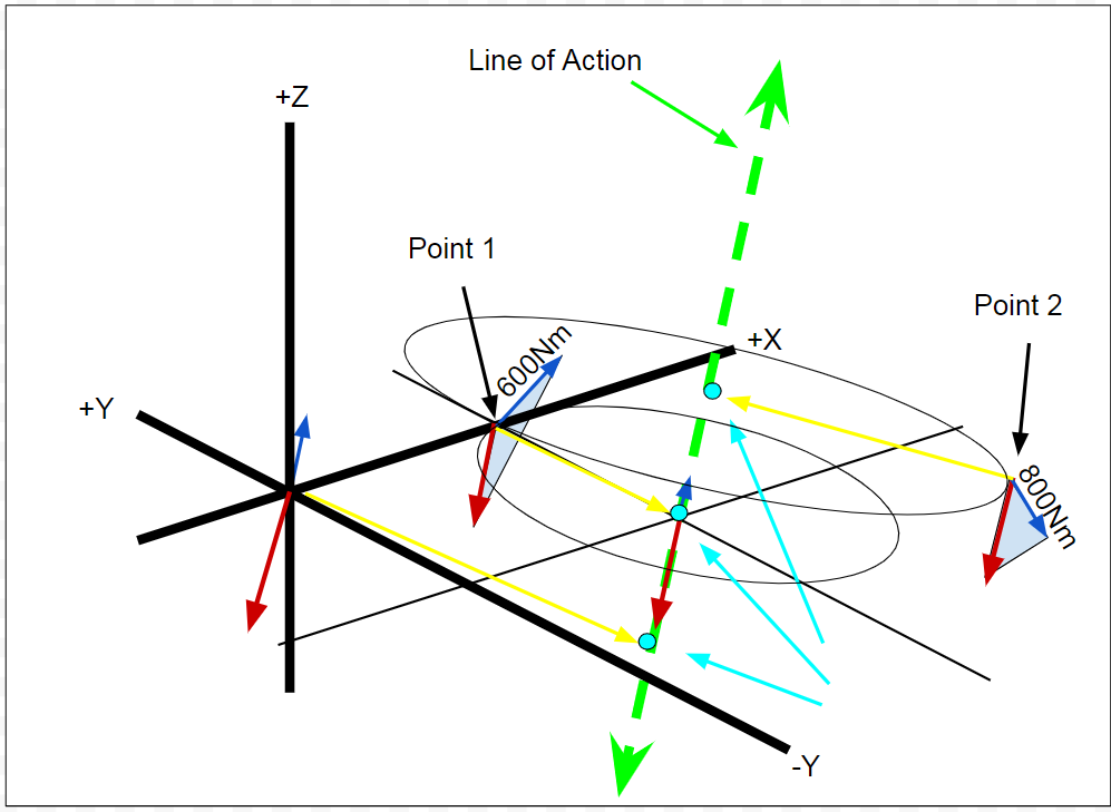
To continue with my attempt at understanding how this works, The following picture shows how the Force and Couple Vectors all have a determinate Vector that point directly towards the line of action for every point P selected in this Force Screw. I believe this is what he means by saying
“Away from the axis the couple vectors always have this same component in the direction of the axis, but they gain increasingly large circumferential components at increasing radii.”
Each Couple vector Tr( P) at some point P, always have one component making up this vector pointing in the direction of the axis.
This can be much easier described by zooming in on the origin, adding hypothetical points 1&2, and the line of action shown below. All determinate vectors, calculated from the Red Force and Blue Couple Vectors point towards the line of action shown in yellow, the determinate vector. Notice that the larger Couple vector of Point 2 also has a larger radius or distance to the axis. This is because the magnitude of the determinate vector is equal to the distance from the axis.
Another thing to note is that based on the Point selected to find the line of action, the determinate vector from that point will intersect the line of action axis at a different Z coordinate shown in light blue. This is ok for now because as the thread describes the aerodynamic forces acting along this line of action and therefore all points along the axis are valid.
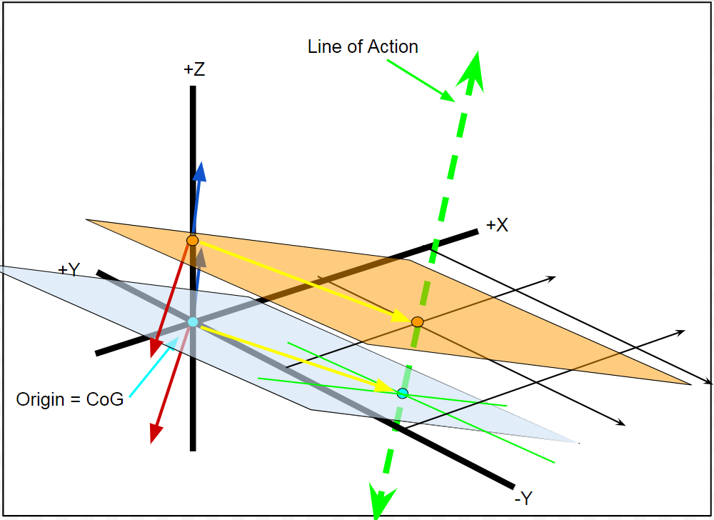
Based on this information we have now found the Line of Action to describe how the aerodynamic forces are acting on the car. This will give us the X and Y coordinates for this line based on the reference frame or plane intersecting the origin. If we base these X,Y coordinates off of a plane passing through the CoG, then we can also find the height coordinate and we will have a theoretical and instantaneous “CoP” for that singular reference plane. However we must be careful how we convey this information as a singular Z coordinate because it is all subjective of the reference plane.
To show this, the next picture depicts the original Force and Couple vectors located at the CoG and the determinate vector pointing towards the line of action. The vector lies along the blue plane with the light blue dots showing where the plane intersects the CoG and the line of action. When taking the measurement for a Z coordinate from this position, it can be seen that the point intersecting the line of action is below the Global X,Y,Z coordinate system plane at (0,0,0).
The orange dot shows where the line of action intersects the global X,Y,Z plane. It also shows the determinate vector and orange point along the Z axis intersection. Also, it can be seen that the line of action is angled towards the Z axis and at some point in space will eventually intersect it. This means that based the Point used along the Z axis to determine the line of action location will not only change the Z value, but also the distances away from the axis in X and Y. This is further displayed through the distance between the Blue dots being smaller then the distance between the Orange. This fact further supports the original theory that there is no center of pressure, only a line of action around which all forces act.
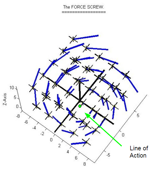
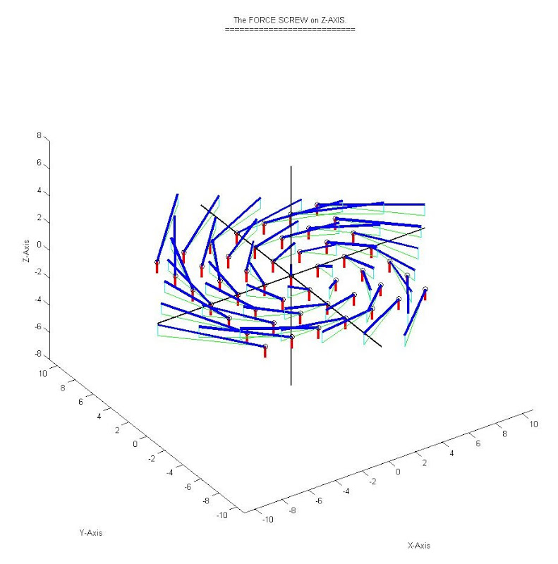
To help reinforce the whole topic, the thread also shows this Force screw from the top of the line of action shown in the next picture. Since we are looking from above the line of action is a dot and parallel to all Red Force Vectors. It is now easier to see how the couple vectors are swirling around a central axis.
Yet another good example is the last picture in the thread which shows the Force screw but from an easier perspective where the Force and Couple Vectors are collinear on the Z axis and at the exact global center. Since the Blue couple vector is pointing in the positive Z direction, all other Couple vectors have a vertical component. The added light blue line is the vertical component of these couple vectors while the green lines are the circumferential component.
I hope someone on the Simscale platform has come across this theory before and is able to help confirm its validity and possibly shed some more light on the correct workings. I have only this one thread as a reference so any help would be much appreciated!