Beckham's rocket kick clocked at 97.9 mph - crossbar impact Part 1: Simulation Tutorial ⚽

AnnaFless · June 24, 2016, 9:05am

Have you ever thought how the crossbar vibrates when a high speed football hits it? How the stresses in the bar propagates?

In 1997, David Beckham while playing from Manchester United side took a historic rocket shot that was recorded at 97.9 mph (~157.6 kph). The ball hits the lower portion of the crossbar and went inside the goal to score against Chelsea¹.

What if this tremendous kick hits directly the crossbar rather then hitting it only on the lower portion? How it will create the stresses and vibrations inside the crossbar?

Let’s have a look via dynamic analysis!

Project Link : https://www.simscale.com/workbench?publiclink=8311230a-1849-4acf-9213-dafd115bb7fc

Click on this link to directly import the project with the geometry into your workspace.

Geometry is courtesy of Ashish Kumar from GrabCAD. Later the goal post was added using Onshape.

Then follow the steps below for setting up the simulation.

Meshing

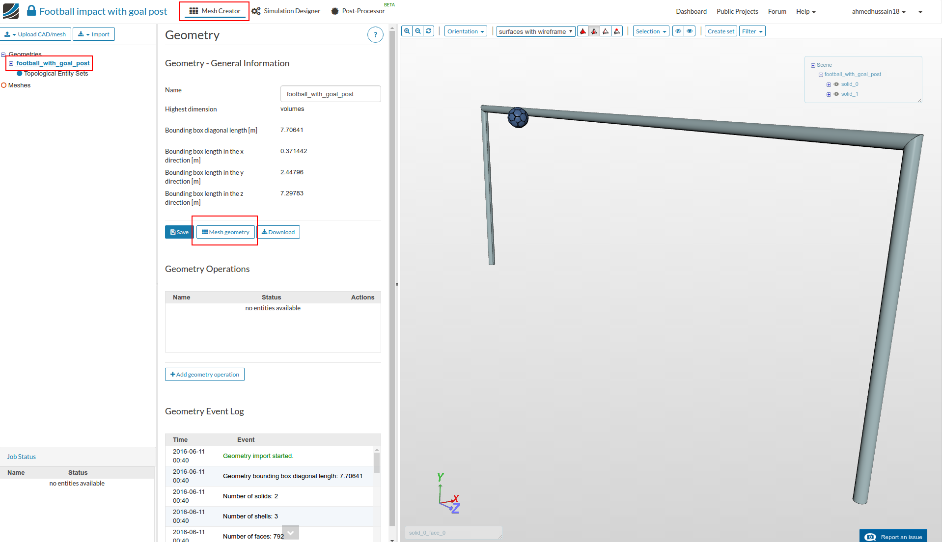
In the ‘Mesh Creator’ tab, click on the geometry ‘football_with_goal_post’
Then, click on ‘Mesh geometry’ button in the options panel.

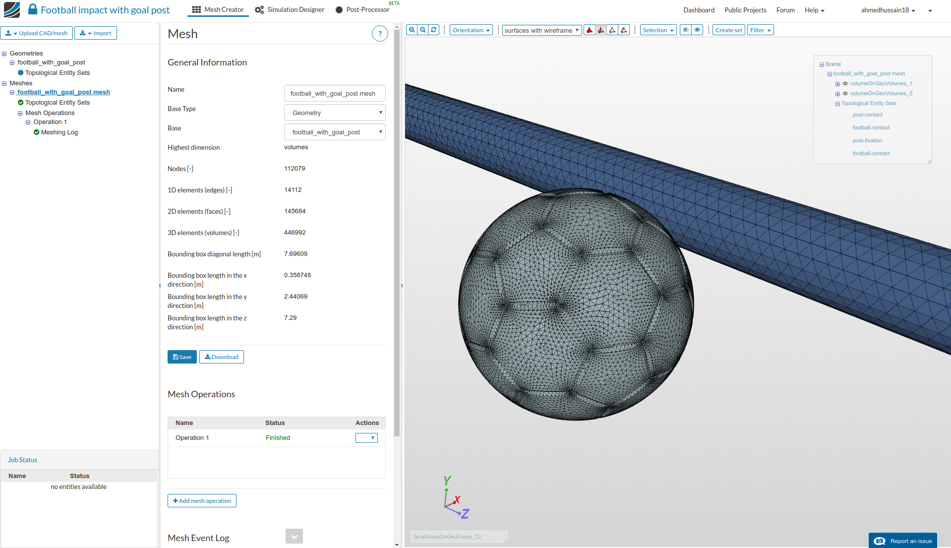
A new mesh operation will be created. Select the first option ‘Tetrahedral automatic’. Change ‘Fineness’ to 1 - Very Coarse and ‘Number of computing cores’ to 8. Click ‘Start’ to start the meshing operation.

With in some minutes your mesh will be ready.

Simulation Setup

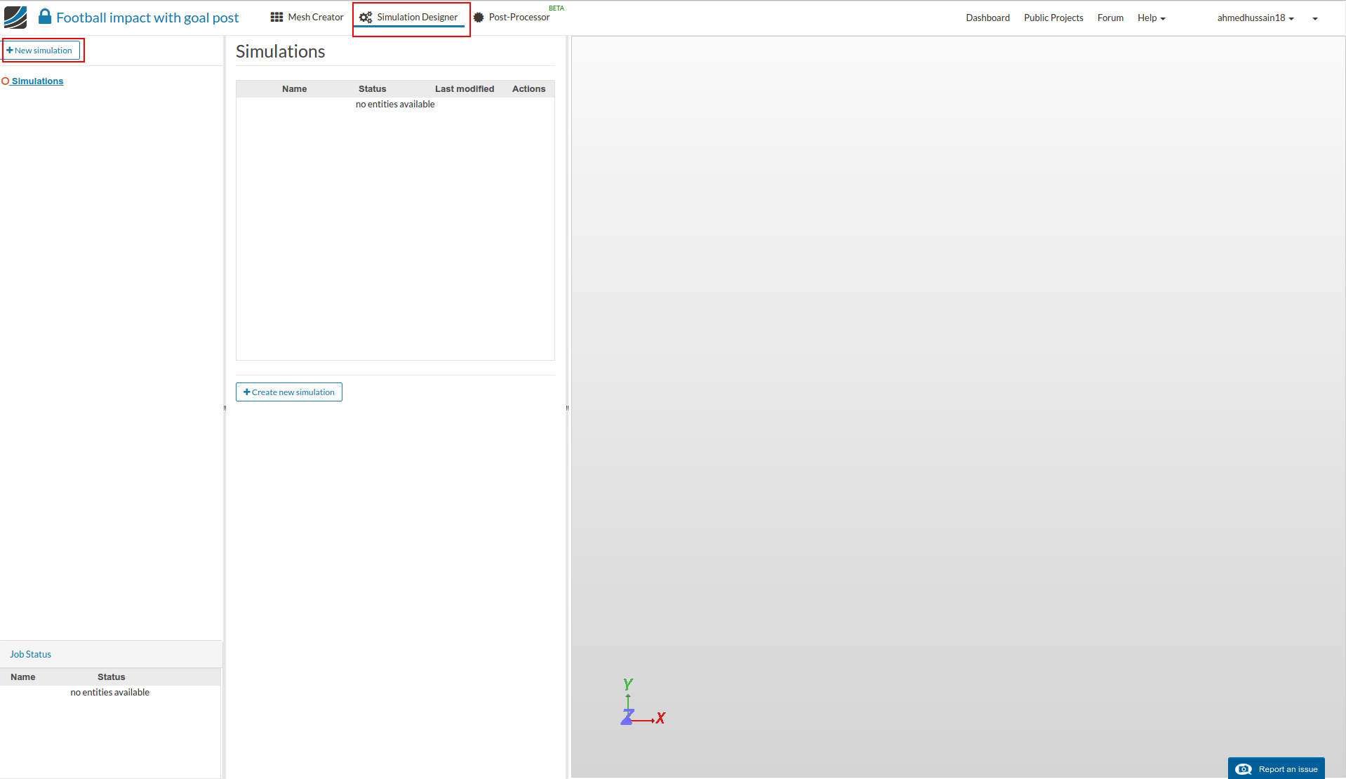
Now to setup the simulation, switch to the ‘Simulation Designer’ tab.

Click on ‘Create new simulation’ in the options panel, give it a relevant name (optional) and click ‘Create’.

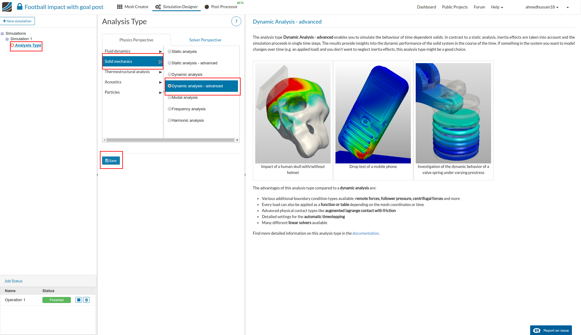
Select the ‘Analysis Type’ options and then select ‘Dynamic analysis - advanced’ under ‘Solid mechanics’ and click on ‘Save’.

After saving, the simulation tree will be generated. We will setup the essential entries required for this simulation.

Domain

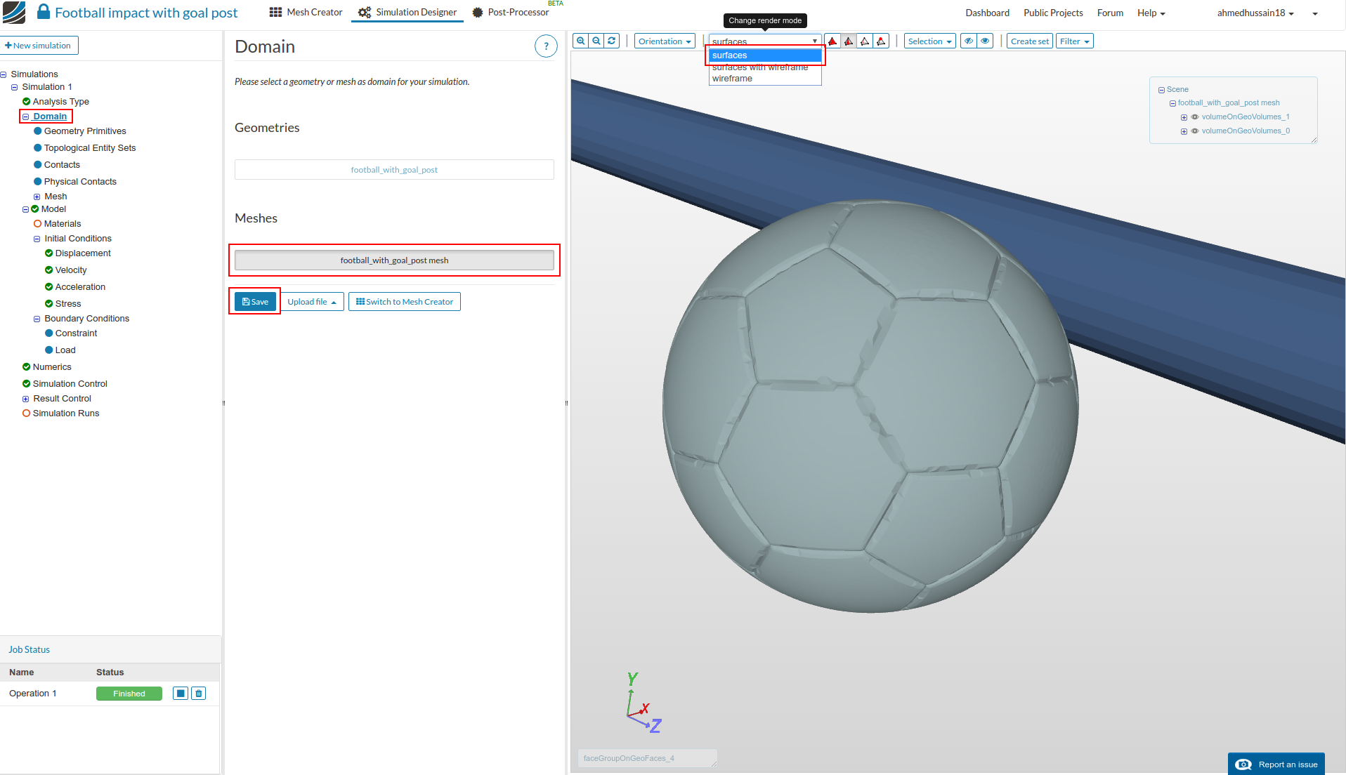
First is ‘Domain’, where we select the created ‘Mesh’. Click on ‘Domain’ and select the available mesh and then on ‘Save’. The selected mesh will automatically load in the viewer. Furthermore, change render mode to ‘Surfaces’ on viewer top to interact with the mesh more easily.

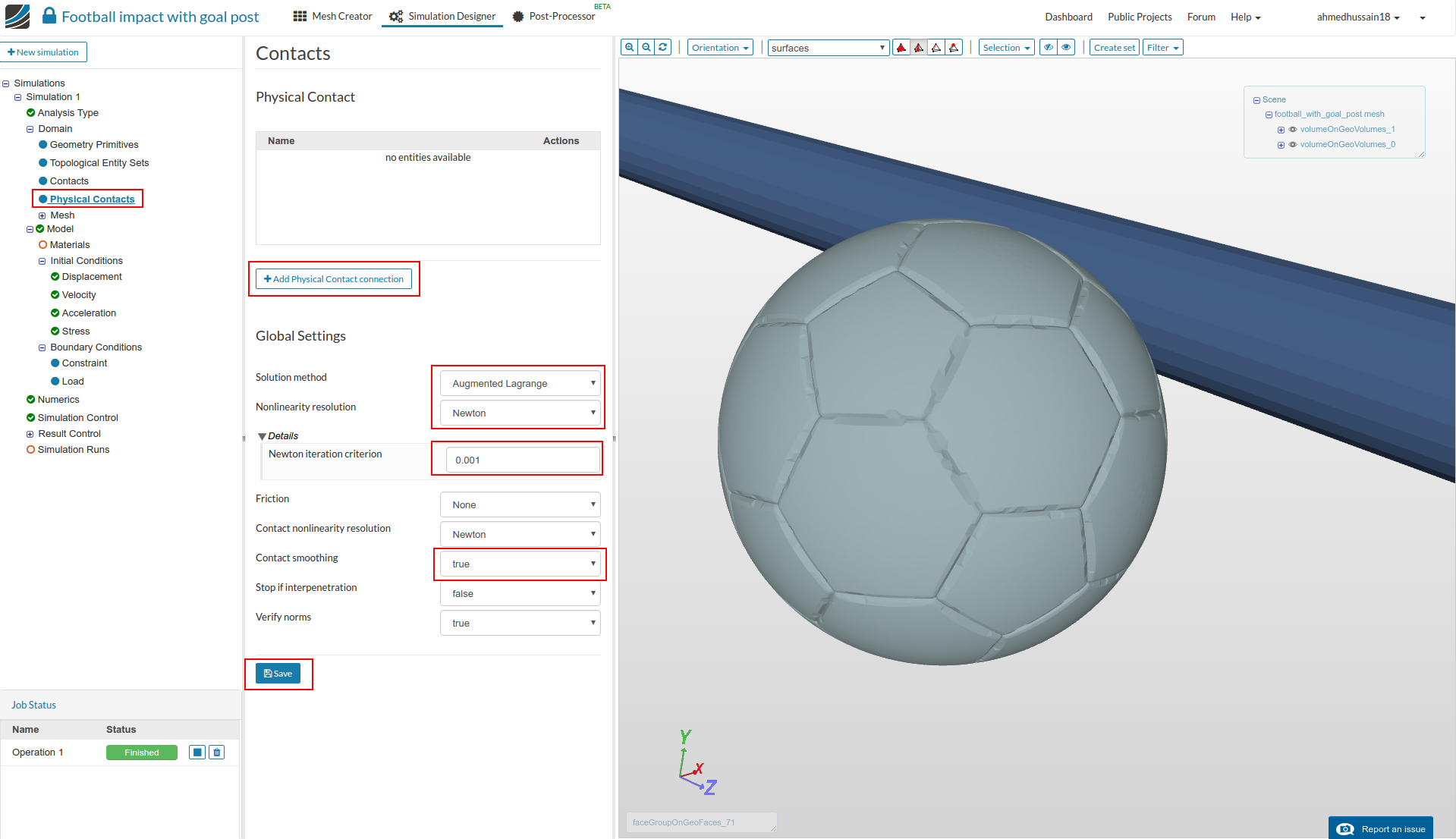
Once you saved the ‘Domain’, an inner domain tree will expand which will have contact options. Click ‘Physical Contacts’, change ‘Solution method’ to Augmented Lagrange, ‘Nonlinearity resolution’ to Newton and change the ‘Newton iteration criterion’ under ‘Details’ to 0.001. Set ‘Contact smoothing’ to true and click ‘Save’. Next click ‘Add Physical Contact connection’ to create a new physical contact.

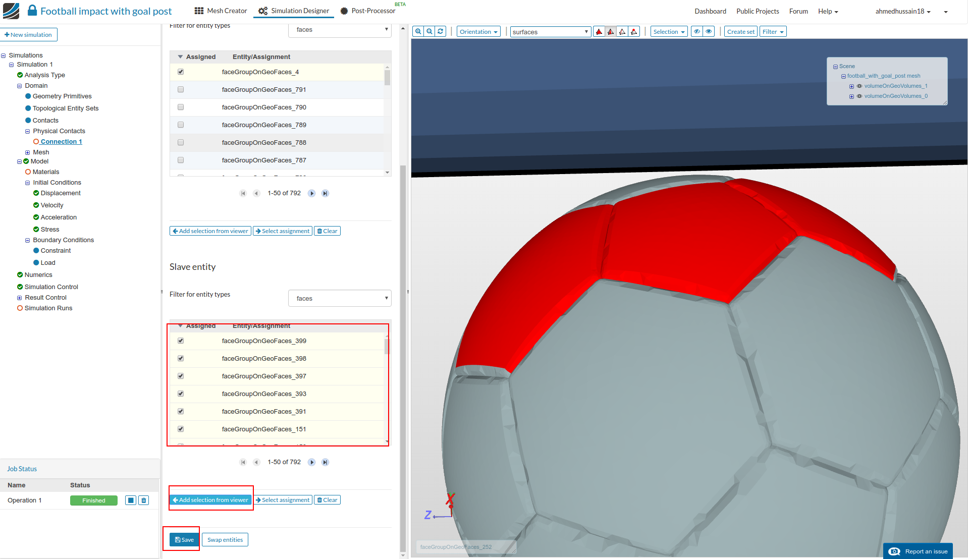
A new physical connection with a name of ‘Connection 1’ will be created. Change ‘Type’ to ‘Frictionless augmented lagrange contact’, select the upper crossbar face from viewer and then click on ‘Add selection to viewer’ under ‘Master entity’ in order to make selected face as master.

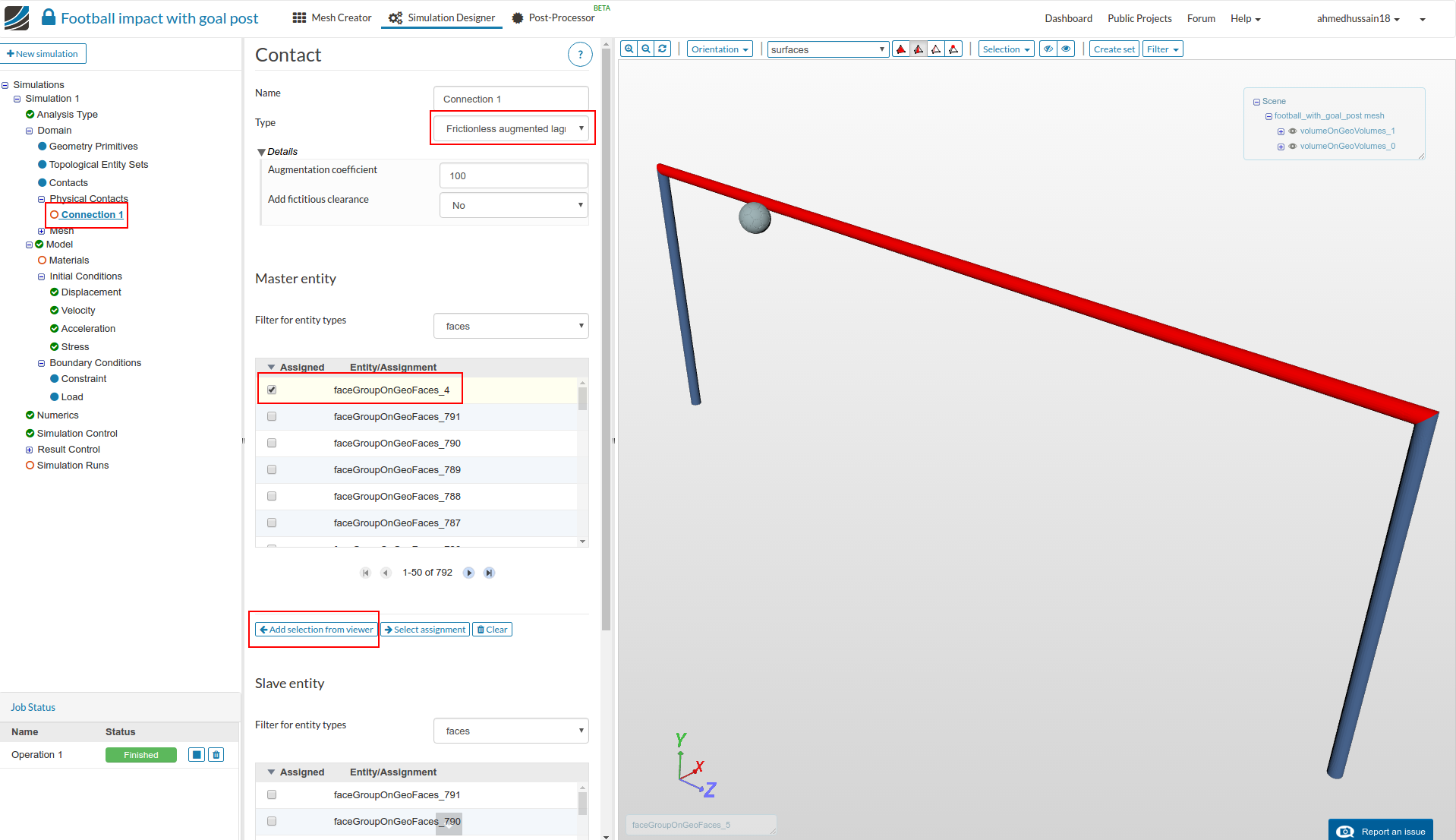
Then scroll down, zoom the mesh and select the following faces as shown in the figure below. Next, click on ‘Add selection to viewer’ under ‘Slave entity’ in order to make selected faces as slave. Click ‘Save’ to finalize contact definition.

Model

Under model comes the ‘Materials’, ‘Initial conditions’ and the ‘Boundary conditions’. We will go through them one by one.

Materials

Click on ‘Materials’ and then on ‘Add Solid material’ in the options panel.

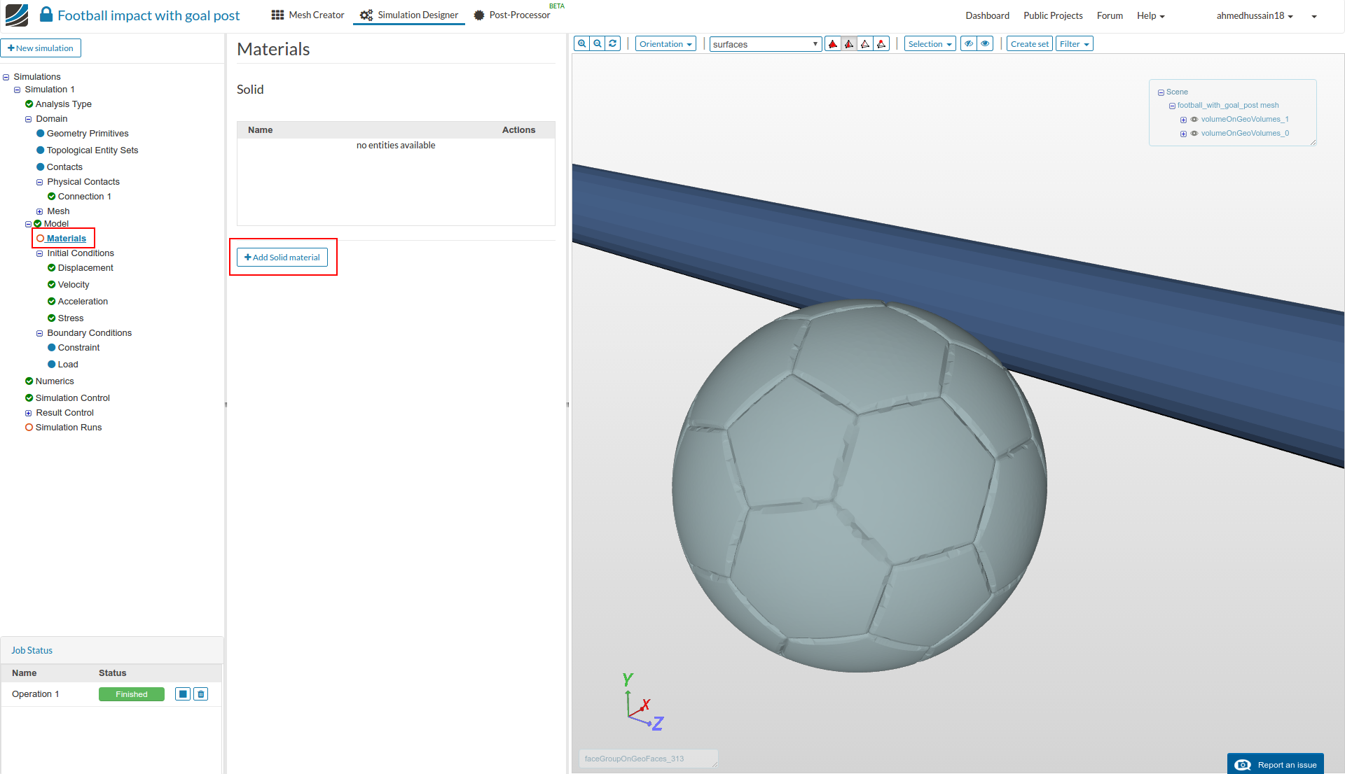
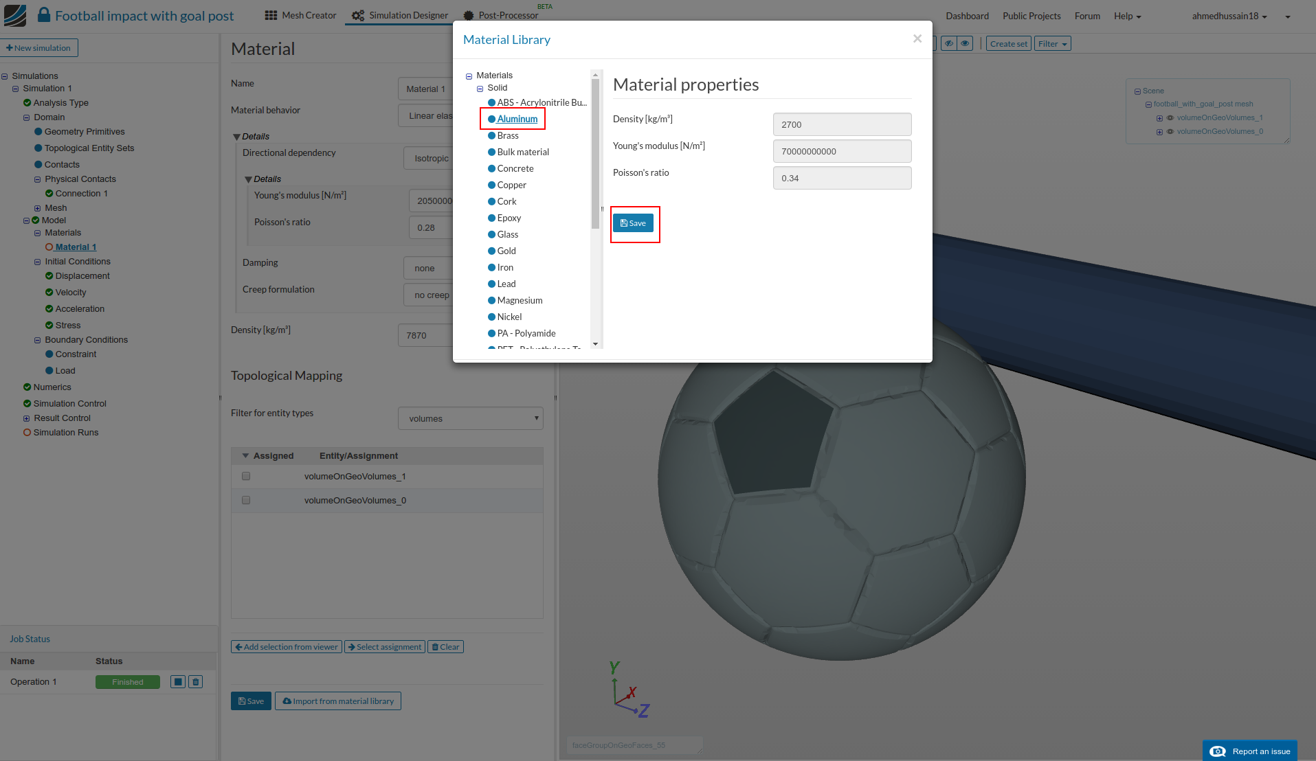
A new material will be created. Scroll down to the bottom and click on ‘Import from material library’

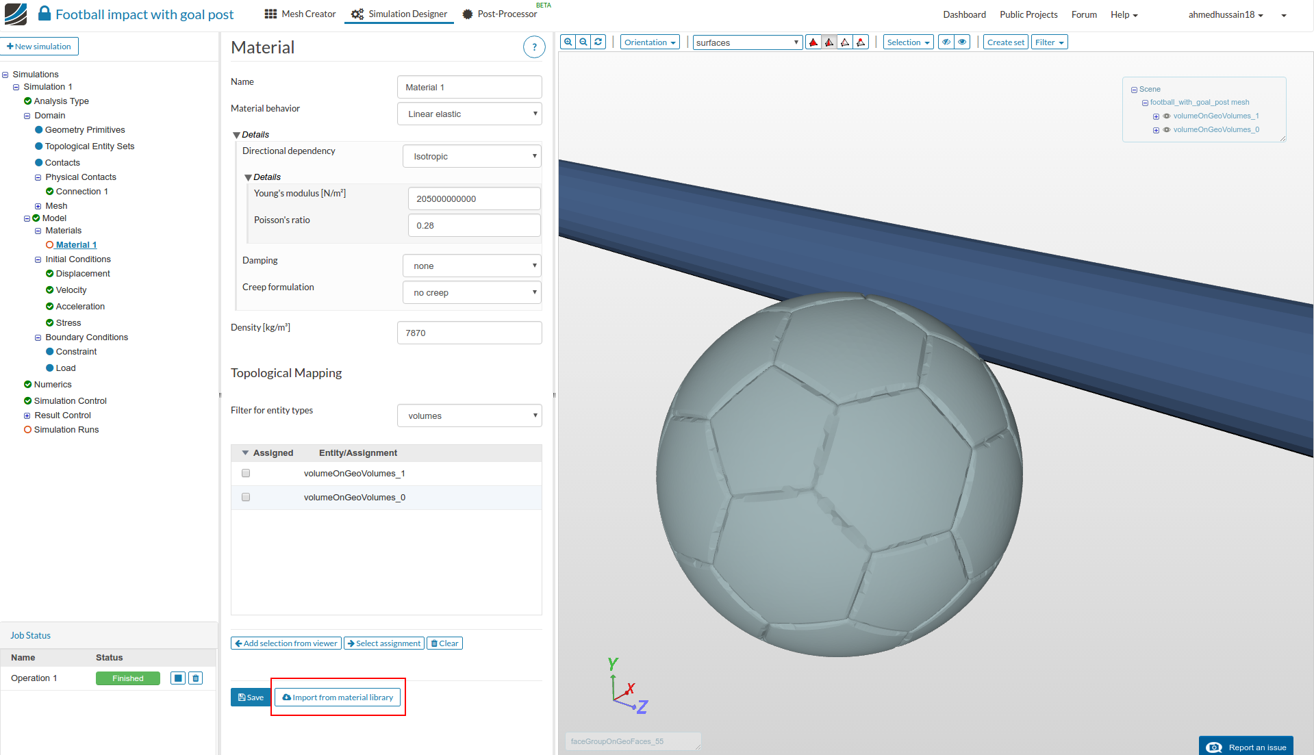
Select ‘Aluminum’ and click on ‘Save’

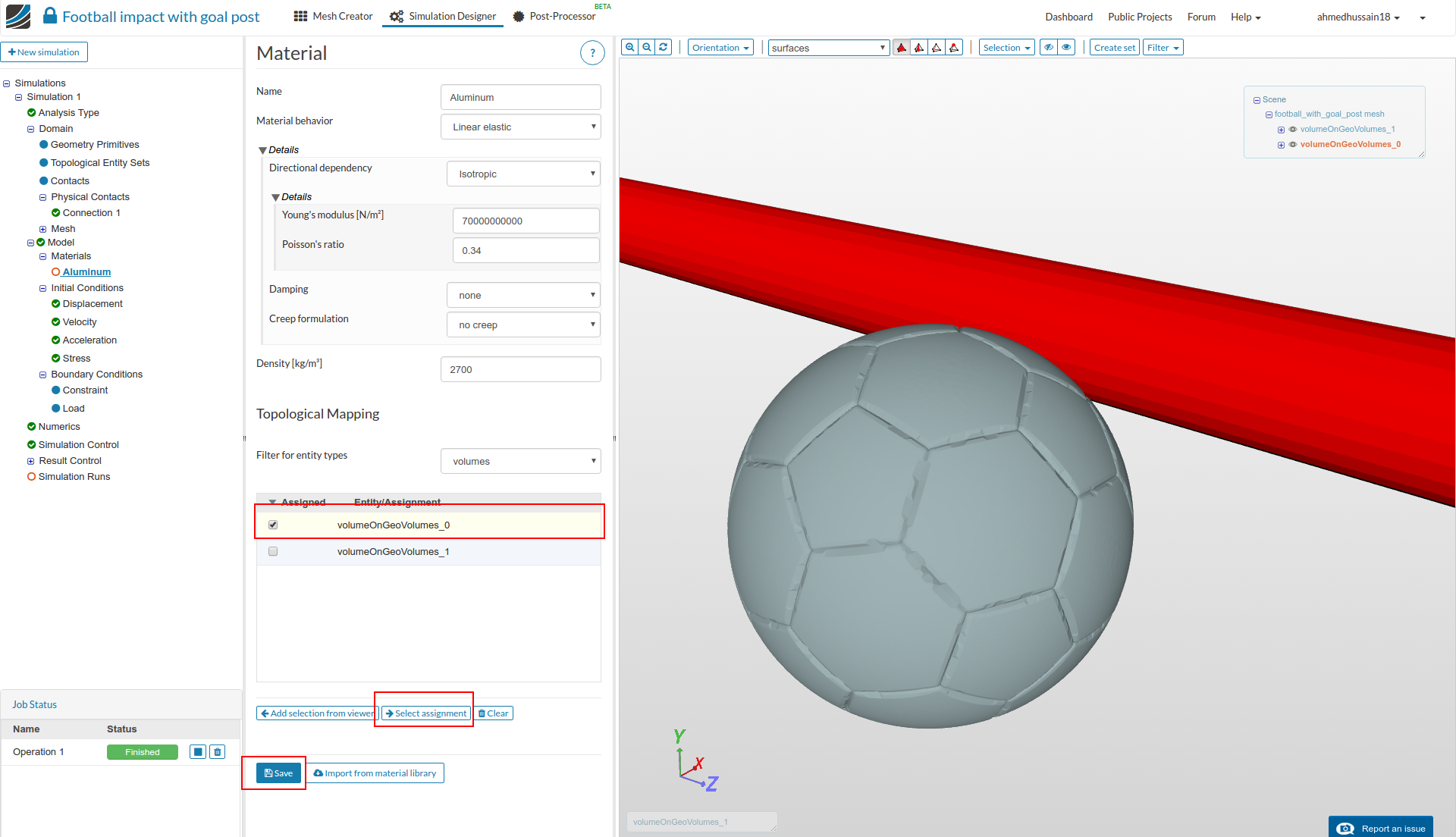
From the ‘Topological Mapping’ list select ‘volumeOnGeoVolumes_0’, click ‘Select assignment’ button in order to make sure that right volume is assigned and then click ‘Save’ to assign aluminum to the crossbar.

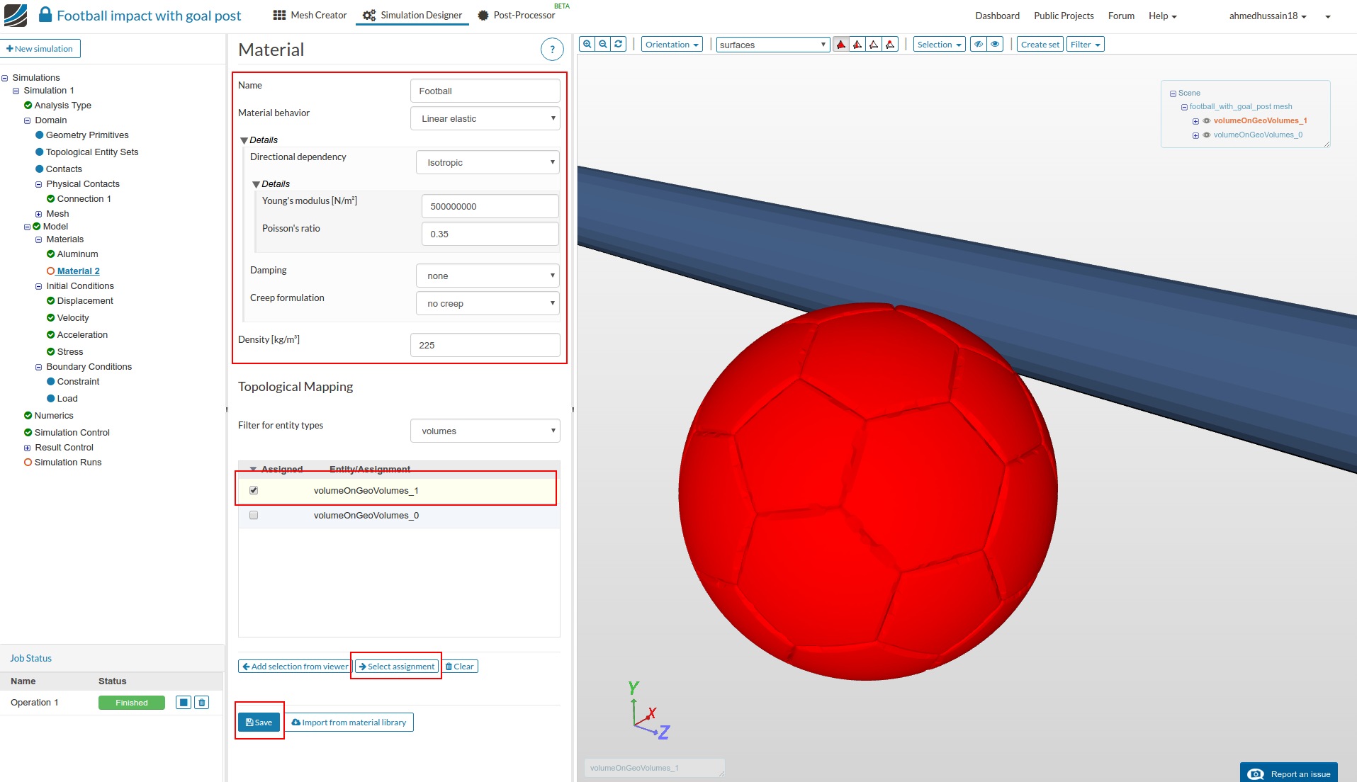
In order to assign material to the football volume, create new material by performing the same procedure and then change the material properties as show in figure below. Rename the material if required. Select ‘volumeOnGeoVolumes_1’ under ‘Topological Mapping’, click ‘Select assignment’ button in order to make sure that right volume is assigned and then click ‘Save’ to assign material to the football.

Initial Conditions

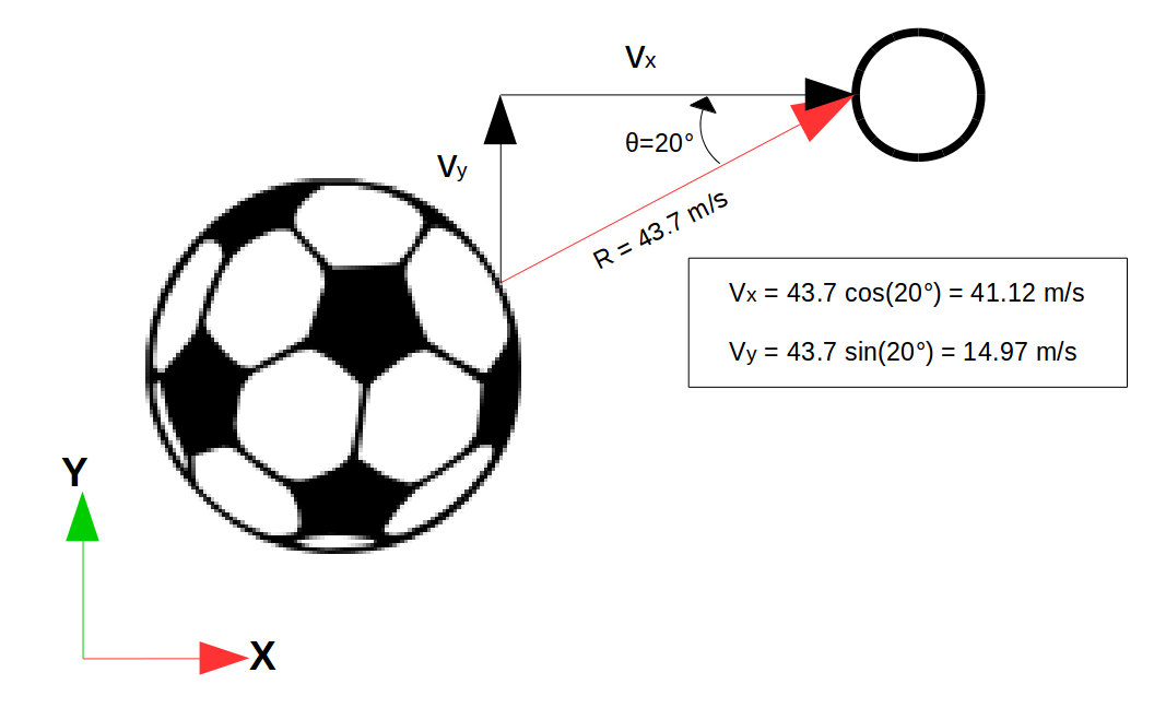
Before we assign the initial velocity to the ball, let’s see how the velocity values are calculated in order to get the resultant velocity equivalent to ~43.7 m/s (97.9 mph). The football is going to hit the crossbar at an angle of 20^o with this resultant speed. Please see the figure below for the calculations.

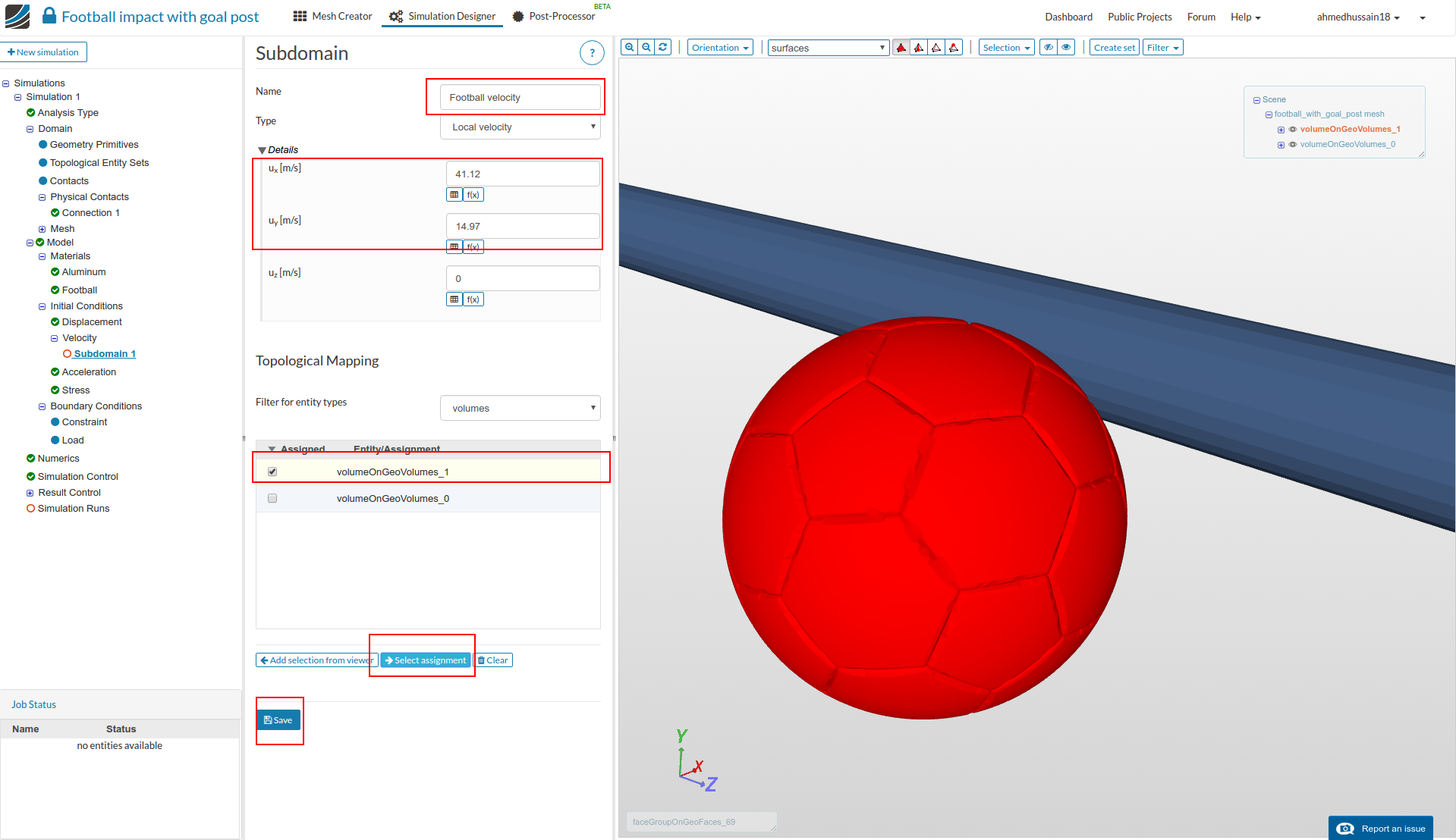
Click ‘Initial Conditions’, change ‘Type’ to Subdomain-based. Click ‘Save’. A ‘Subdomain’ section will open below. Click ‘Add subdomain’ to add initial velocity for a specific domain.

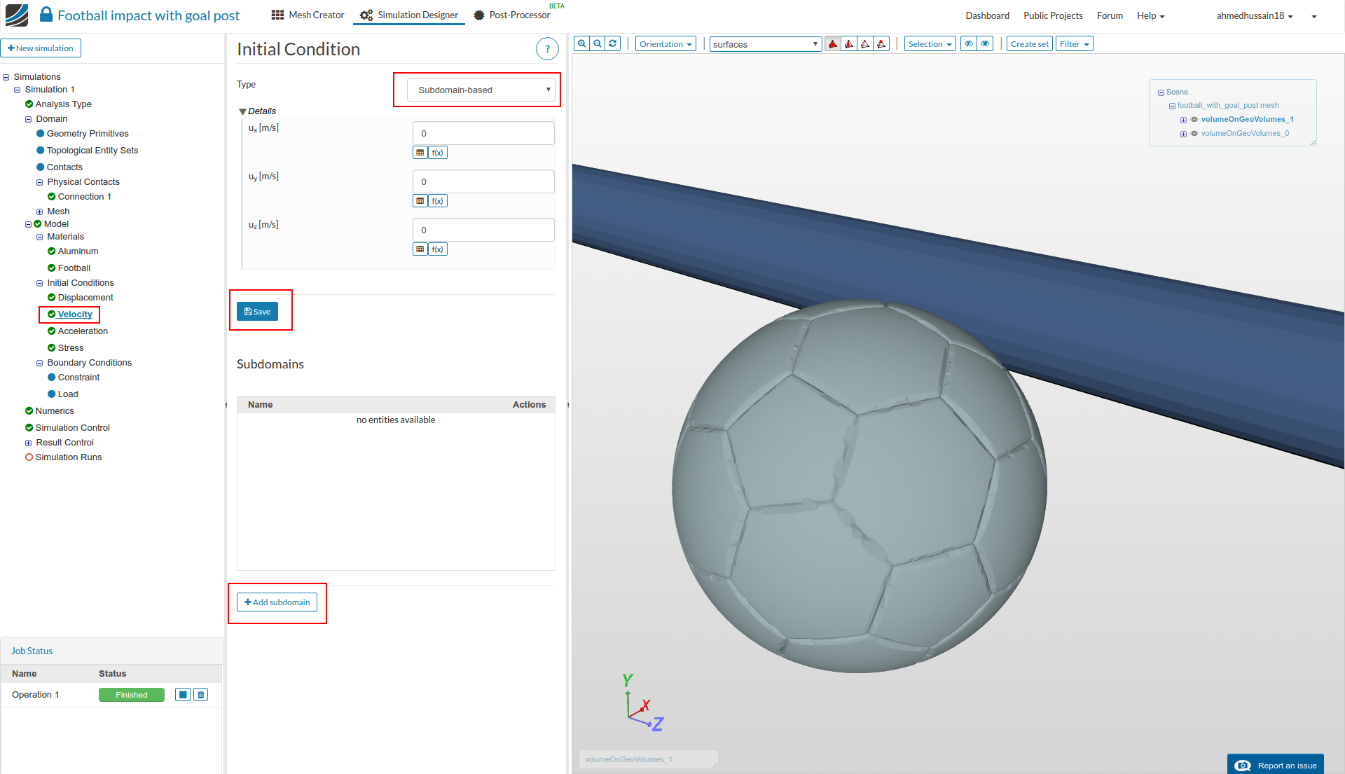
Rename the ‘Subdomain’ (optional). Change the values of ‘u_x’ and ‘u_y’ as shown in figure. Select ‘volumeOnGeoVolumes_1’ under ‘Topological Mapping’, click ‘Select assignment’ button in order to make sure that right volume is assigned and then click ‘Save’ to give the defined initial velocity to football.

Boundary Conditions

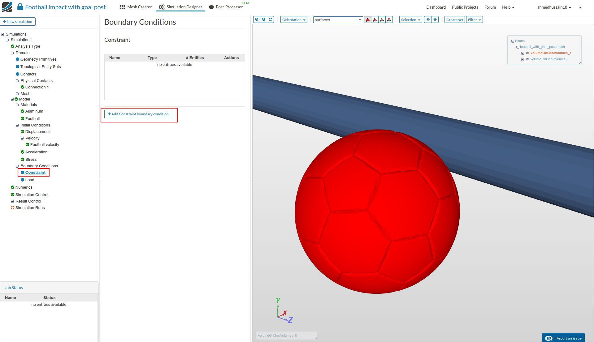
Now we have to fix the goal post. Select ‘Constraint’ from tree and then click ‘Add Constraint boundary condition’ to add the boundary condition.

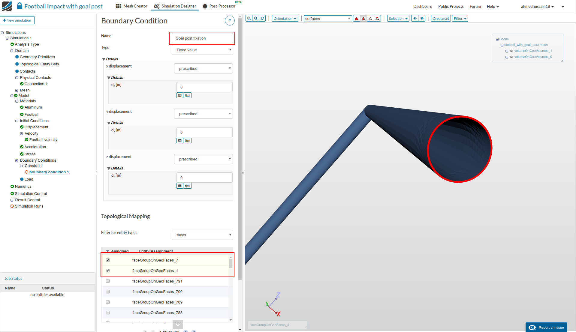
Rename the ‘Constraint’ (optional). Zoom out the mesh in viewer and select both ground surfaces of the goal post. Click ‘Add selection to viewer’ to add the selected faces in ‘Topological Mapping’. Make sure that you are in mode before you select the faces. Scroll down and click ‘Save’ to save the constraint.

Numerics

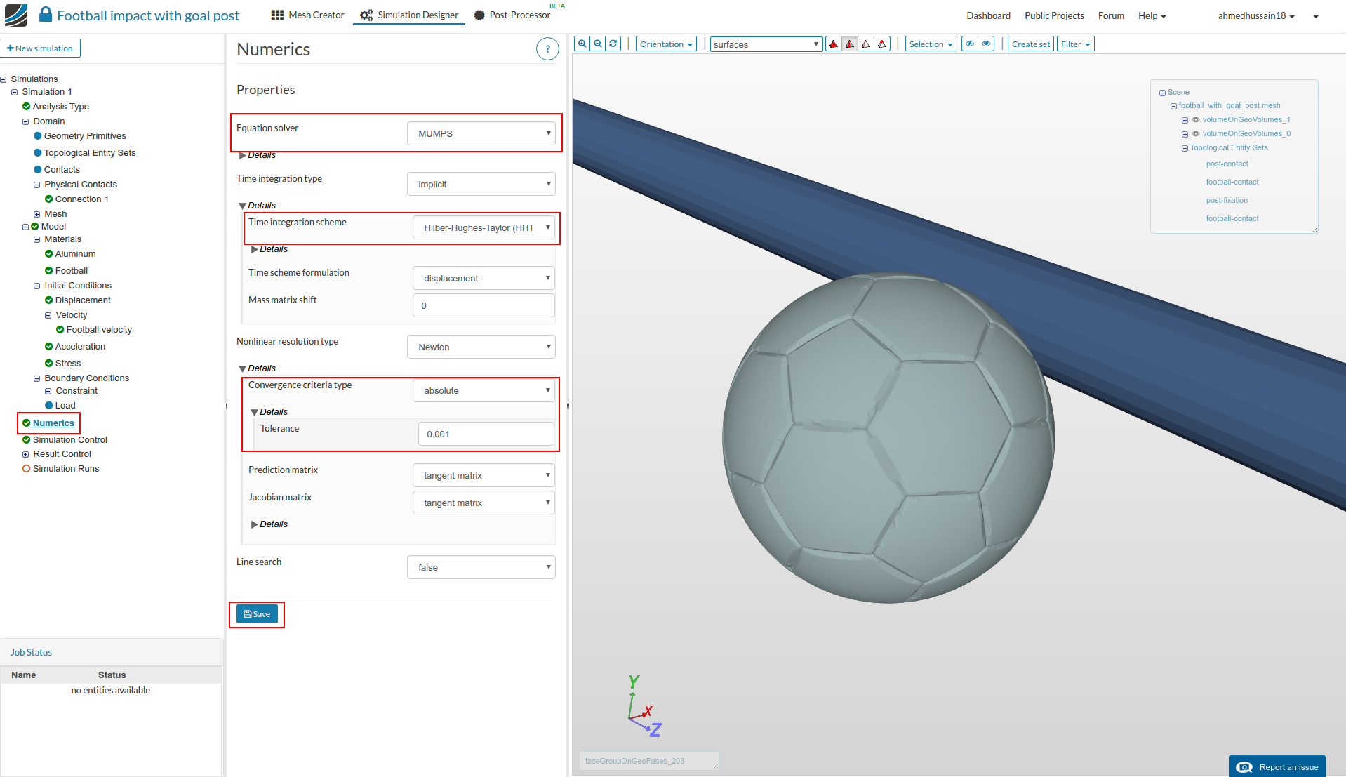
Click ‘Numerics’ in tree. Change ‘Equation solver’ to MUMPS, ‘Time integration scheme’ to Hilber-Hughes-Taylor (HHT), ‘Convergence criteria type’ to absolute and change ‘Tolerance’ to 0.001. Click ‘Save’.

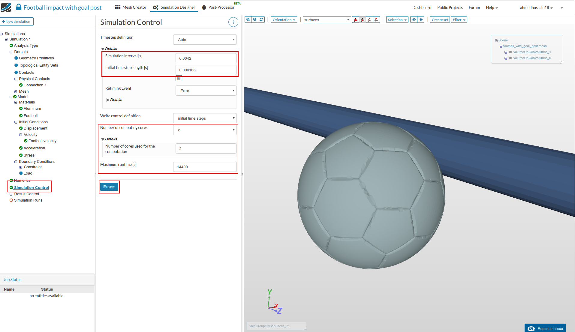
Simulation Control

Click on ‘Simulation Control’ in the tree. Change ‘Simulation interval [s]’ to 0.0042, ‘Initial time step length [s]’ to 0.000168, ‘Number of computing cores’ to 8, ‘Number of cores used for the computation’ to 2 and ‘Maximum runtime [s]’ to 14400. Then cllick ‘Save’.

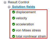
Result Control

Expand ‘Result Control’ under tree and delete ‘cauchy stress’ ‘Solution fields’ since it’s not require and thus some simulation time will be saved afterwards.

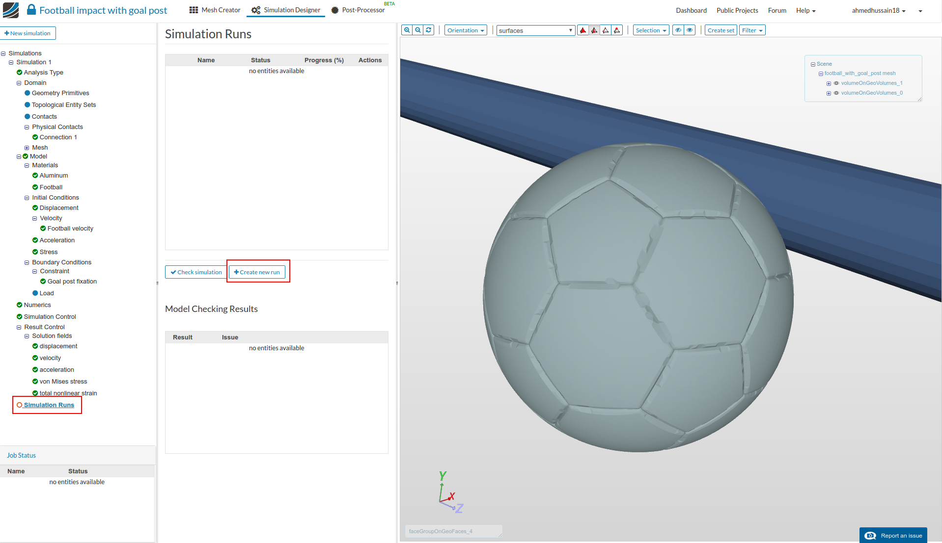
Simulation Run

Click ‘Simluation Runs’ in the tree and select ‘Create new run’. Ignore the warning that pops up by clicking ‘OK’. Rename the run (optional) and then click ‘OK’ to create a new simulation run.

Next click ‘Start’ to start the created simulation run.

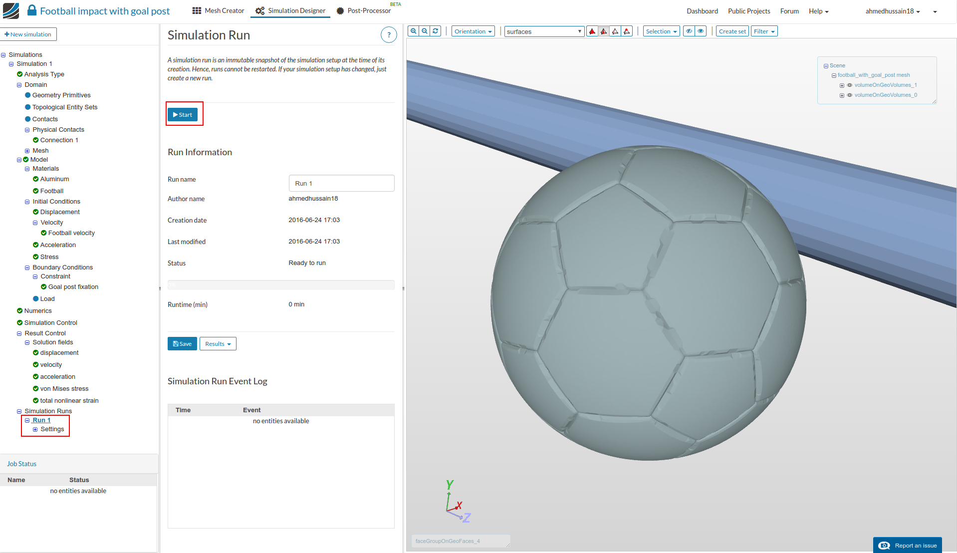
The simulation run will take approx. 60 mins. Once it is done the status will change to ‘Finished’.

For post-processing, please see HERE

References

[1] The 5 fastest shots ever recorded in Football