Ok, you are starting to convince me 
In the meantime I tried a laminar flow assumption on the NON layered mesh with air viscosity 0 (I was trying to stop rotation) but that only got the Cd by CFD to be only 320% bigger than XFLR5.
I will try the 0-time look at NON layered mesh with potential flow initializing and report back.
2D is next
BUT for sure my eyes are opened and are seeing for sure why XFLR5 type programs should not be relied on for real life 3D situations about drag…
Sorry Daren but I do not see anywhere to set up a potential flow initialization. Where to find?
I looked in ‘Initial Conditions’, ‘Velocity Inlet’ of ‘Boundary Conditions’ and just about every less obvious place  .
.
Also, would you suggest Laminar as turbulence model?
What do you think of making the walls on the geometry as slip walls?
I have not found a quick way to check cores hours for a mesh and simulation, are they just listed at the end of the Meshing Log (ie Finished meshing in = 29.93 s) and Solver Log (ie ExecutionTime = 578.18 s)?
Hi Dale,
you can find this via your Dashboard when you go to the top right drop-down menu clicking “Manage Account”. There you can see every project with the amount of core hours used.
Is that what you wanted to see?
Jousef
I have looked at that in the past but have not been able to see what I did, right after I do it.
Also, is was sorted weird as a default.
Then when I sort by start time, at this current the last operation shows as ‘2018-08-03 9:41:37AM’ while my current time is ‘2018-08-03 7:04:02PM’ . It seems way too dated for my use.
My Dashboard under ‘Latest jobs’ says I last did a job at ‘Start: 8/3/2018, 12:39:07 PM’ which is likely correct, but there I can not see core hours.
I would like an instant way of seeing core hours preferably in the WB for meshing and simulations.
Dale
This option is found under simulation control, initialise with potential flow = true. A note on this option, it takes longer for the solution to initialise so expect a long wait before the simulation starts
Laminar basically presumes no turbulence, and unless you are very sure this is the case, it is rather unlikely to be true everywhere in the domain. K-omega SST has traditionally been the most accurate, but the K-epsilon is useful if you are having some convergence issues.
This would mean that boundary layers on the surface are neglected, this is unlikely to produce accurate results. Slip walls are primarily used on the bounding box surfaces, but they do have other uses.
Cheers,
Darren
When you answered 2nd and 3rd questions, did you remember that we are not trying to be accurate here but we are trying to duplicate what XFLR5 does by using irrotational inviscid flow? I would think anything that makes CFD simulation ‘forget’ about boundary would help with an apples to apples comparison.
3rd point, yes, I believe xfoil, the underlying code uses some kind of wall treatment, I might be wrong but I do remember ticking a box in xflr5 for boundary layers, but that was a long time ago.
2nd point, I am not sure if it is entirely applicable, turning of turbulence wouldn’t make the flow irrotational, nor do I believe it should affect the potential flow calculation.
Also, I am not sure we could get an apples to apples simulation, hopefully, we could get close. Not sure what the apples to apples simulation would achieve? We want similar results sure, but not necessarily using similar techniques (and full circle to the 2D thing  )
)
BTW, have you seen this project?
I am trying to make one last ditch effort to get an apple to apple in 3D. Yes I saw that project but it does not take into account wing tip effects nor planform taper.
What this is turning into for me is not a question of how accurate CFD is but to determine how different XFLR5 3D results are when CFD is used with ‘same’ governing laws, so to say (just can’t think of a better way to say that right now  ).
).
If I can get CFD to give nearly the same results as XFLR5 in the above situation, then would that not validate both programs somehow?
In any case Ali’s project certainly means I have no reason to do a similar exercise on my airfoil.
But if we cant then which is correct? and if we can, but we have removed everything CFD, are we comparing it to CFD?
On the contrary, Ali’s project proves that results are comparable, as long as the mesh is sufficient and all boundary conditions are correctly defined. Run yours as 2D, compare to experimental of xfoil, and they don’t match, we know they can, and that the correction is something we can do. Get it right in 2D and up the complexity.
Just my thoughts good luck!
Then I get to have more fun  finding out why not the same.
So by Ali, we see that CFD sufficiently predicts a ‘standard’ airfoil shape to wind tunnel results but does not compare not CFD results to xfoil results. And then, I have seen lots of tests showing that xfoil vs wind tunnel results are good. So this means your 2D test is not needed doesn’t it  ?
?
Darren @131890
There is a ‘Viscous’ checkbox which I do have checked but I did find this quote about XFLR5 and viscous calculations (from Guidelines for QFLR5 v0.03 1/58 October 2009) :
'5.11 Viscous and inviscid calculations
-
In VLM and panel methods, an inviscid analysis/polar may be defined, in which case there is no need to define a polar mesh for the foils. The viscous characteristics will be set to zero.
-
The LLT is necessarily viscous.’
And also this quote from the same document:
As is generally the case when transposing 2D results to 3D analysis, the estimation of viscous drag is probably too low and may lead to arguably optimistic results.
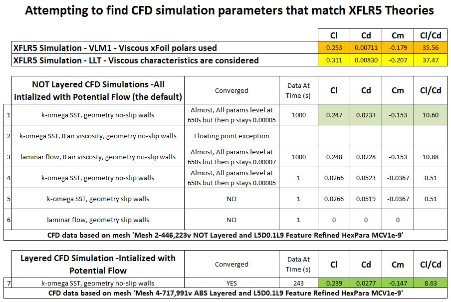
In any case, I have run an LLT simulation in XFLR5 and added its results to the chart below:
So, we were not able to come up with parameters that match XFLR5’s theories, your best guess was line item 4 I believe.
I think it is time to conclude that I should only use CFD from now on for 3D aerodynamic analysis of total drag. I wish I could verify the the actual total drag of this wing was close to CFD but I believe it will be, even though CFD predicts that the total drag is nearly 4 times what XFLR5 predicts.
Do you think that my conclusion is supported by the results of this topic?
Thanks,
Dale
That quote to me justifies the findings and conclusions you have stated. If we are going to be strict and base our conclusion on evidence from the comparison I would probably state the conclusion as:
The findings demonstrate that lift predicted is somewhat comparable between xflr5 and CFD, with the CFD prediction showing a slightly lower lift value with comparable viscosity settings and xflr5 showing higher, and as described and supported by the quote:
optimistic results.
This conclusion is evident in drag also, where the drag present in the CFD simulation is much higher than that predicted by xflr5, without any data on the experimental results, the difference could be a range of things including the above mention of optimistic viscous results, CFD turbulence modelling, mesh refinement (until a mesh independence study proves otherwise) or uncomparable boundary conditions between CFD and xflr5.
end
I think that is the limit of what we can draw I think your statement on drag accuracy is fair, but we cannot say from the evidence we currently have, in this topic/simulation/review of documentation that CFD is better than xflr, but more a suggestion that it is true, and this would be in my opinion enough to act upon
Awesome project and a great contribution to the forum for future reading.
All the best,
Darren
Excellent expanded summary!!
But now I have to figure out what that is
I can give you a brief description and its relevance:
When creating a domain for a problem (meshing) we split the fluid volume (in CFD) into smaller cells, the solution is created by solving the numerical problem in each cell. In real life this is an infinite problem, however we split it into a finite one (CFD is the finite volume method) however the closer to the infinite problem we are, the more accurate the solution will be, at the expence of computational requirement. A mesh independence study basically runs the same setup but with different size meshes, the coarsest mesh is expected to have worse result than a fine one, and the simulation wich has the least cells but a finer grid (sorry, or mesh) will not produce significantly better results is the mesh independent result.
This can be performed starting with a really coarse mesh, and increasing the number of cells by 1.5 in each direction and running again, when you have a few meshes (say between 3 and 5) you can plot the results (for your quantity of interest, in this case, lift, drag and lift over drag would be ggod quantities) vs mesh size (volumes) and determine the cheapest mesh when the results steady out (you would expect the results to be flat lined between the last two meeshes at least if the independence study is sufficient) and then we would use that grid for further studies.
Another technique is to run two meshes, determine the difference between them in paraview, and refine those areas. This is only quicker if you know how and once again would need some experience and time invested into paraview. I would consider the first method as the best practice.
Best,
Darren
So, would the easiest way to get the 1.5 times increase in cells be by multiplying the number of cells in the background bounding box x,y,z directions by cuberoot(1.5)?
Sorry, to be clearer multiply the number of cells in each direction by 1.5 this would increase mesh size by 1.5^3 but any less and it would be hard to detect change, your right, this would increase mesh size rapidly as this compounds with each mesh.
No problem I guessed that, did I read it wrong, or did you fix it
Darren, @1318980
So I have been working on the independence study but I need some advice.
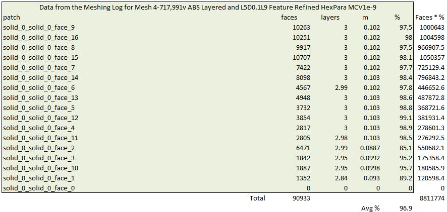
Here are my results so far, with the base data for the plots in the lower table (published results so far are the green row):
I have stopped because I think that the average % of total layer thickness achieved in the top chart is skewing my results. As you might realize, I had a very hard time throughout this topic to be able to obtain even the 97% inflation value for the mesh I have published so far. Unfortunately, when I either increase or decrease the # of volumes away from the 97% mesh, the resultant meshes are not layered as well. I am not sure I have the stamina to tweak % inflated value for all the meshes that I need for the Independence study so that they match the 97% I achieved in the published mesh.
Can you make any conclusions from the above interim independence study?
Dale
PS here is how I calculated % Inflated (weighted):
Hi Dale,
The %inflation business might actually make sense to decrease as cell sizes get smaller, the reason being, if the cells at the wall are no thicker than the defined thickness (in inches in your layer inflation) then there is no need to inflate a layer. The Y+ values for the 82% inflation should be checked, if they are still in a good range, let’s not worry.
Presuming all are converged, I would say not yet Mesh converged. if you find the local refinements are too much, you could reduce them (this will skew current results so if doing this you could make a second line called local refinement reduction) and do the same process.
Interesting that cd is reducing almost linearly.
Let’s go 1 or 2 more refinements maybe and re-evaluate? Check Y+ first though just in case.
Best,
Darren