XFLR5 vs CFD

DARN ‘p’
I see that a lot stuck at 0.0001…

Yep, its a pressure based solver so it is normally last to converge. But it doesn’t mean to say that is not converged if the results are steady and continuity good, we can say its converged.

1 Like

Yep, I’ve seen stable values as low as 100s so I assumed that they were good.

Good to know that it is OK to assume that… :slight_smile:

1 Like

I have fired off some simulation on the project I just shared with you, one looks ok the others look stuck also. I am logging off but will update you as soon as I am back on. Again, apologies.

Are you kidding, thank-you? I know how you spent your Monday evening :upside_down_face:

Well things really started going well after you left.

I got rid of everything but the Geometry in the project and I created 4 versions on my new Mesh 1 that has been tweaked with your 7 parameter suggestions:

  1. Change the ‘Max face aspect ratio for layers’ from 0.5 to 2
  2. Change the ‘Max ratio of layer thickness to medial length’ from 0.3 to 0.9
  3. Change the ‘Min face weight’ from 0.02 to 0.002
  4. Change the ‘Min volume ratio between neighbouring cells’ from 0.01 to 0.001
  5. Set the Inflation parameter for 2 layers instead of 3 while maintaining the same overall sum of all layers thickness using the same expansion ratio of 1.1.
  6. This changed ‘Thickness of the Final Layer’ from 0.03821 to 0.06
  7. Decrease the ‘Minimum overall layer thickness’ from 0.02 to 0.0002

I adjusted the Background Mesh Box dimensions slightly.
I added a Mid-Volume Cartesian box to refine an area outside the wing to Level 2 (to help with the isovolume errors that were found).
I used the same Whole Wing Region box to refine the wing to Level 5 as before.
I then used a further 'All Surfaces refinement ’ to Level 8 instead of the Feature Refinement I used initially (this got rid of the refinements at each wing rib.

I then ran simulations on all 4 versions of Mesh 1 and a further Full Resolution Simulation on ‘Mesh 1-1,239,387v 32x16x16’

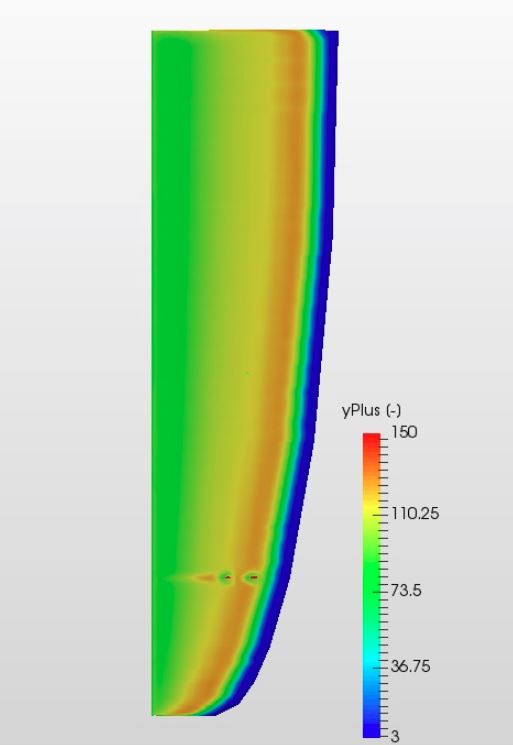
I looked at yPlus range on simulation ‘0aoa Mesh 1-1,239,387v 32x16x16’ and it looks pretty good I think (would like comment on this please, seems a little low on leading edge):

So then I just put the results in this new chart:

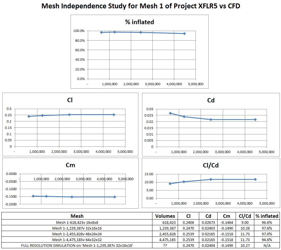
Darren, which mesh would you say to use for the definitive CFD results, the converged values or Full Resolution values?

Also, could you do your Paraview isovolume error check on the results?

I will put this data into a final XFLR5 vs CFD comparison chart once we are happy.

Anything else I should do except have a beer now :smile: :beers:

Thanks
Dale

P.S. Now after all that trouble, is there a way to make images that show where the boundary layer precisely separates at this 0aoa and 135mph case (not just particle tracing, maybe like a separation line)?

3 Likes

Hi @DaleKramer, sorry for such a late reply. In short, lovely results!

From these results, meshes of around 2.5 million do not significantly differ from that of 4.5 million, and there for the mesh independent results can be obtained from either but the cheapest would be the 2.5 million cell mesh.

On the topic of full res vs wall function, I looked at the results and saw that there was no significant difference between the two (correct?) and therefor doesn’t matter, for simplicity, stick with wall function. To be thorough, you could run a full res simulation with a mesh which has a y plus of around 1 all over, in theory, this should also be identical in results since it would be proving that the modeling of the boundary layer is a correct assumption but don’t think there is any point making extra work for ourselves.

Sure, I’ll download the results now.

Hmmm, not sure, can you maybe upload an image of what you mean from google maybe? Then I could say for sure. Does the BL separate at this 0AoA?

Best,
Darren

1 Like

Well, I was just querying because the Full Res is not the same as converged, it is the same as the Not Full Res simulation of the same mesh that the Full Res was made from (ie 1,239.387v) and I think it is a significant difference.

I was thinking a line on the surface of the geometry that shows a line of S points from this image:
separation1

That is what I want to know (and see in 3D), I am sure it does behind the trailing edge and maybe a little before the TE, but how much :slight_smile:

Maybe not a line but just a surface color for attached (green) and detached (red).

And then show some nice little particle traces in the air around it :smile:

Dale

Darren @1318980

What do you think about that blue leading edge in my yPlus range image?

Dale

Sorry, I re-read this several times, I think my brain has shut off. To clarify, the same mesh run in full res and wall model are significantly different? which simulation/runs can I look at, maybe I looked at the wrong ones.

Oh yes, I think doable, never done before but doable. So I think by doing a dot product on the surface tangents with the near-field velocity, those that face the ‘wrong way’ we could highlight as -1 and those the correct way as 1 then visualise with a surface colour map between -1 and 1. This needs paraview, I think we should test on one with definite separation where visually we can see the recirculation. Any chance you could run one at say 15 degrees AoA? or do we need more for this foil?

Well, this ties in with the full res simulation. If the results are significantly different then the Y+ in the blue is an issue I would say, but if not then it doesn’t matter.

1 Like

AHA moment… so you are saying that BECAUSE the full res results are same as not full res on the same mesh, that the layering is GOOD.

I thought that the full res would give the best converged results, sorta like a mesh with infinite cells could do somehow, but full res was not used all the time due to excess core time to do it.

I think I understand now, a dangerous thing :smile:

I think at even maybe 12 degrees would show separation sorta between LE and TE, 15 would show close to LE.

I will make a geometry for that as I really don’t like the standard way of changing air inlet vector (but that is another topic :smile: for you to convince me it is OK to change inlet vector without undue wall influence (especially high aoa’s)).

This is fun :wink:

Dale

Haha! well as long as you use an inlet-outlet condition all around the wing its fine, I could link you an example?

Best,
Darren

But what if the air that gets to the wing has already been influenced by some air that was already bounced off a ‘wind tunnel’ wall in front of the wing? (maybe I should see your example but the ones I have seen made me question the method)

Here is my NACA0012 project, it’s my playground for trying weird things so excuse the mess. The best example is validationMK2, to get an idea of setup (ignore the failed runs :slight_smile: )

But essentially the walls above, bellow, upwind and downwind are set to inlet-outlets, where they don’t ‘know’ about what lies outside them (such as surrounds or wind tunnels) they ‘know’ that air is travelling in a direction that is going into the domain, if flow exits the domain, then it acts as if it just moves out of it, to us that is zero gradient. So there will be no deflection from any wall external to it, nor will the walls themselves make the flow behave any differently to if they were orientated with the flow.

1 Like

Maybe that wall setup should be called an open door instead… :smile:

It is so nice to able to do things here that can’t be done in the real world :smile:

I will duplicate your wall and inlet setup and run a 12aoa simulation :slight_smile:

Thanks,
Dale

Haha, yes, a true ‘controlled environment’ I would describe it as :joy:

I just noticed also you were getting errors saying that the instance ran out of memory. This is because you are saving too many timesteps. Since we are only interested in the converged results, if you set it to run to 1000s then the time write intervale can also be 1000s saving only the final results, this saves download time, and allows the most significant data to be saved. When I view your project, it says you saved every 1s, and ran for over 300s and only saved 38 steps before running out of space, so I don’t know what data is present, however, I would guess its the first 38 steps. Does that make sense?

1 Like

Yes it makes sense I thought I was still just using default values for simulation control, I thought I would figure it out later, I guess now is later :slight_smile:

I was caught by the hidden ‘Details’ dropdown on the write value until now…

I will correct.

How is the ‘Adjustable Runtime’ write control any different from ‘Timestep’?

RE: NACA0012

  1. Why are there 2 symmetry ‘walls’? Does this simulate infinite span?
  2. How do you make those symmetry ‘walls’ act like inlet/outlets for some sideflow in air inlet vector?
  3. And the big question… why cant I input my air velocity vector as magnitude and angle about each axis? It is dark ages to me to have to break my vector down into x,y,z components on a calculator, or am I missing something?

Thanks,
Dale

This to me makes more sense when thinking about a transient simulation time steps would be the number of steps between the written times, whereas the adjustable runtime is the interval between written steps in seconds, one is a number the other is a quantity of time. for steady state with a 1s interval, 1000s = 1000 timesteps so both are the same.

Yep exactly :slight_smile:

ooo, bit tricky that one. I think the best solution would be to make a periodic boundary condition between the two for my case, for your case (a non 2D shape) we couldn’t do that, full geometry would be needed removing the symmetric assumption.

The only ease there would be that we don’t have to calculate, we would then require 4 inputs, not 3. But I suppose it makes sense to offer this as an option.

Best,
Darren

So is this why my runs were hanging yesterday, writing results every second?

I must have unknowingly changed it thinking it would do as I expected, not hang the run :slight_smile: