Recording
Aerospace Workshop II feat. EUROAVIA (Session 3) ― Vibration Analysis of a Jet Engine
Exercise
Have you ever thought that what exactly will happen to the jet engine if one of the fan blade breaks out? It will rather produce vibration due to overall change in center of gravity of a jet engine. But how much it will vibrate? In this exercise we will be looking in to the vibration of the jet engine due to blade loss.
The cutout of the jet engine geometry used in this exercise is shown in the figure below. Only the outer cowling (with strator and struts) and pylon are taken for this analysis, whereas the internal whole jet engine and wing will be ignored since we are only interested in the impact of its vibration on to the cowling via strator and struts.
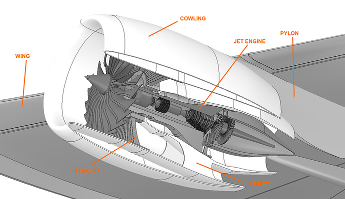
- The base model for whole assembly except the internals of jet engine is provided by Aisak from GrabCAD .
- The base model for the internals of jet engine is provided by Goutam Das from GrabCAD .
This exercise focuses on the vibration study of the jet engine cowling due to missing single or multiple fan blades. First, a frequency analysis will be performed in order to get the natural frequencies of the the model. Next, harmonic analysis will be performed on a specific frequency range of interest with the missing blade vibration load in order to see at which frequency the vibration will be highest. Harmonic analysis produces a sinusoidal load through which one can detect the peak displacement value at a specific frequency. The model with missing single and multiple blades are shown in the figure below.
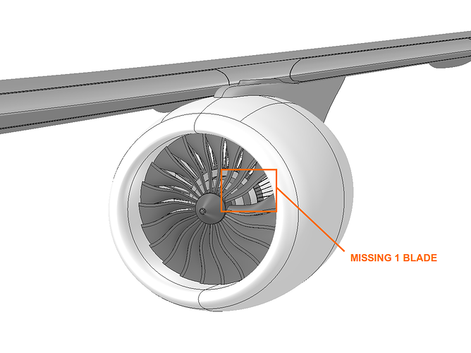
Jet engine assembly with 1 missing blade.
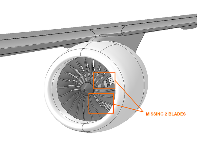
Jet engine assembly with 2 missing blades.
The different combinations for performing the simulations are:
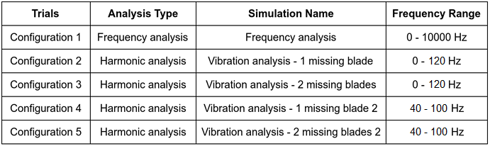
Please note that separate simulation needs to be set up for each configuration
Step-by-Step
Import the project by clicking the link below. (Crtl + Click to open in a new tab)
Click to Import the Homework Project
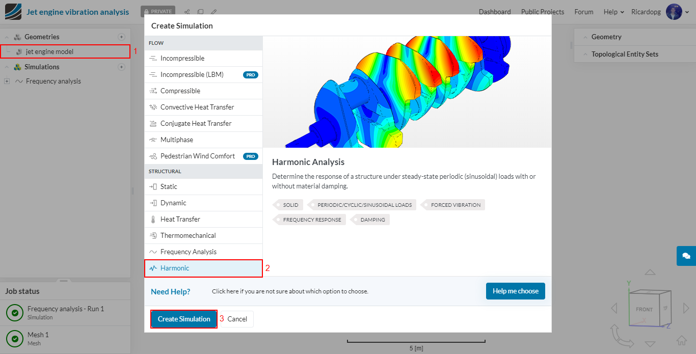
We will start off by clicking on the geometry jet engine model and then on Create Simulation.
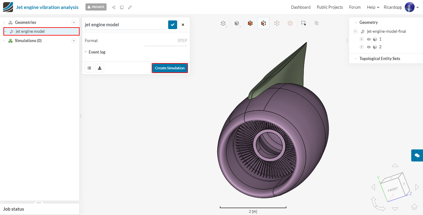
For the first simulation, we will choose a Frequency Analysis.

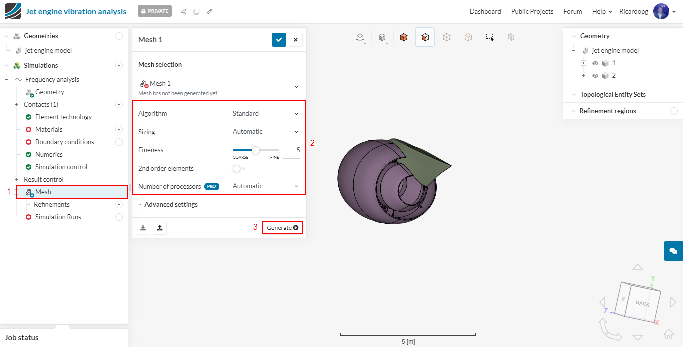
Meshing
In the simulation tree, navigate to Mesh. The Algorithm will be Standard. Furthermore, change the Fineness to 5. Afterwards, click on Generate to start the meshing operation. The number of processors is automatically chosen by SimScale to optimize the usage of core hours.
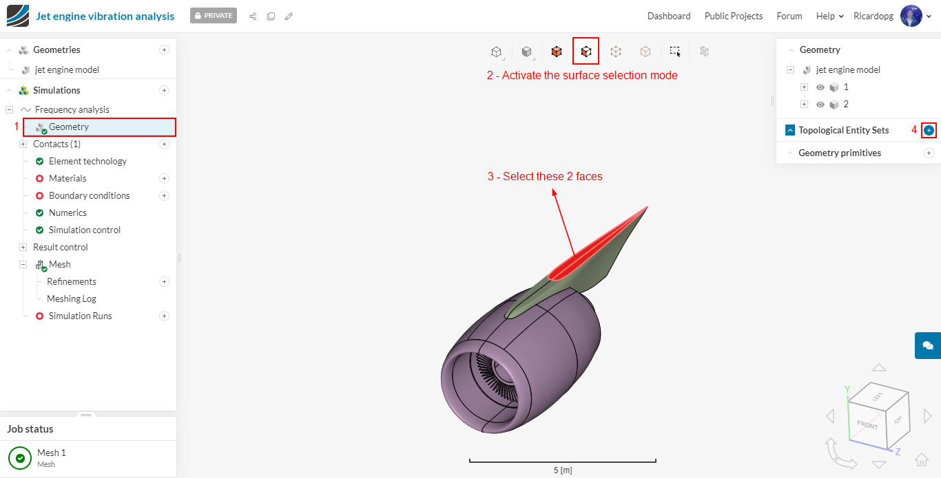
Now it’s time to create topological entity sets. These will help us to assign boundary conditions later on.
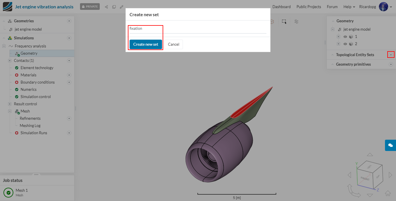
To create a new set, follow these steps:
- Make sure the Geometry is selected in the simulation tree;
- Select a surface or surfaces that will constitute the new set;
- In the right-hand side panel, click on the + icon next to Topological Entity Sets;
- Name your set as you seem fit.
The first topological entity set will be named fixation. It consists of the fixed supports:
And then name this set as fixation:
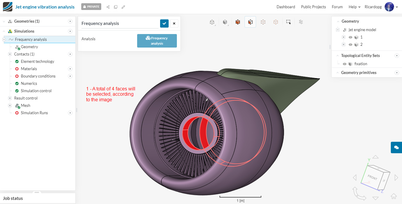
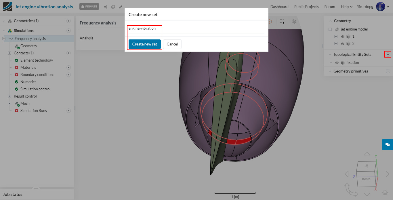
The second and last topological entity set will be named engine-vibration. The 4 inner round surfaces of the cowling will be selected:
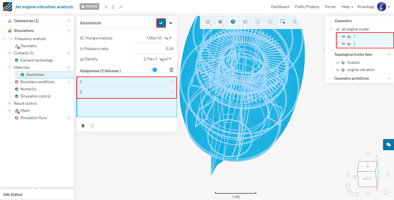
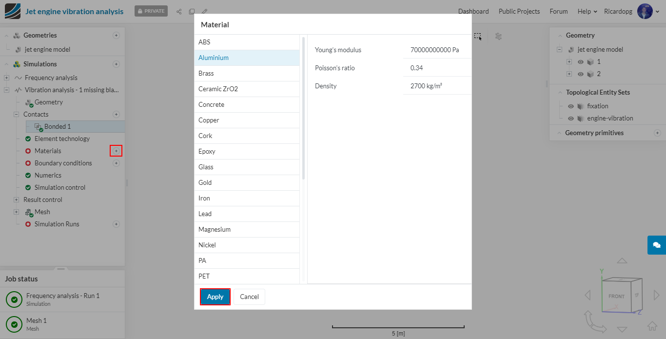
In the simulation tree, navigate to Materials. From the list, select Aluminium and hit Apply.
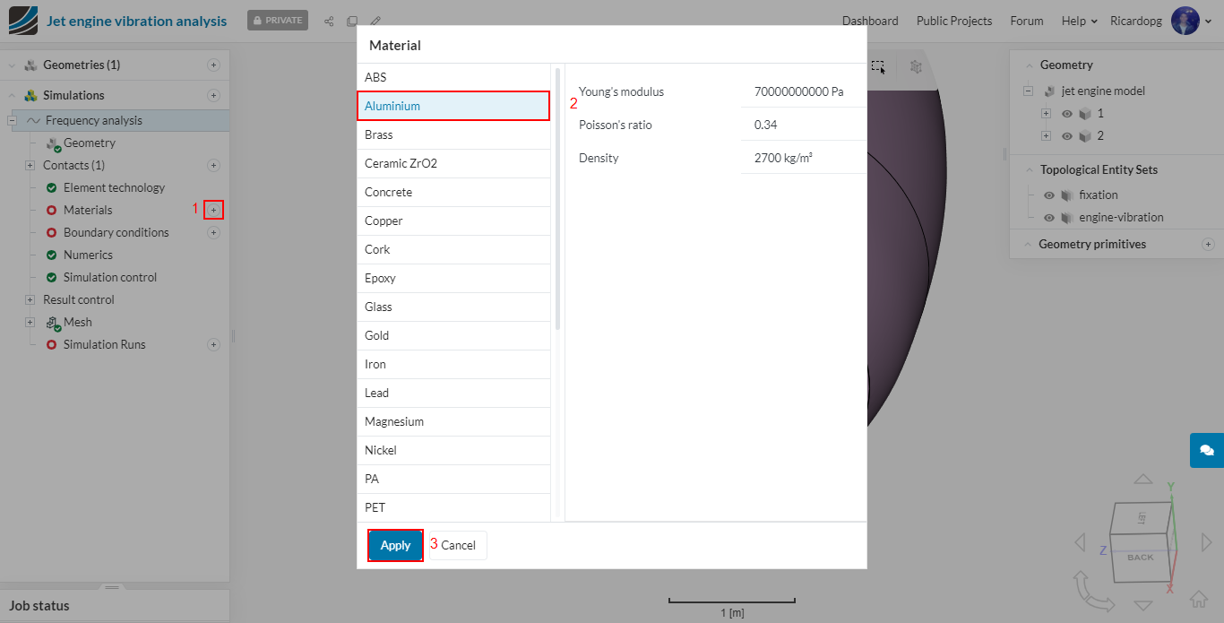
Assign it to the two volumes (1 and 2), then click on the blue mark to save.
Boundary conditions
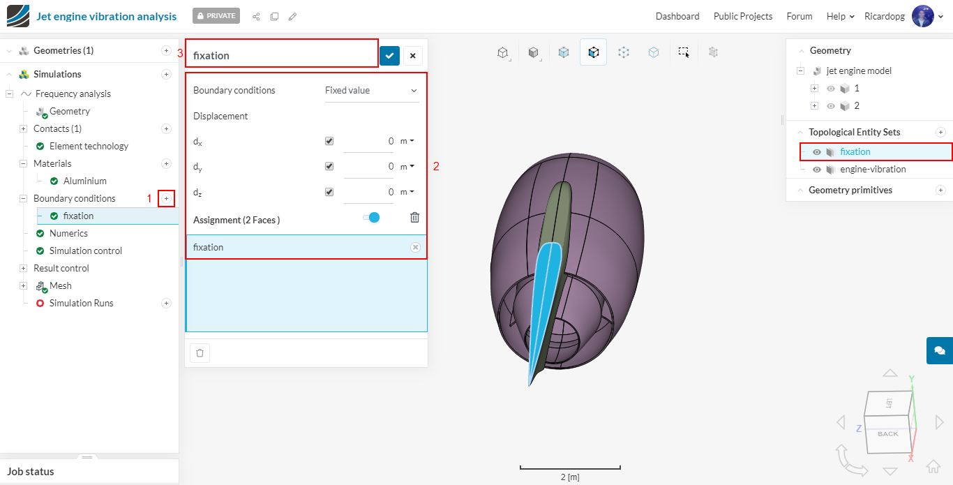
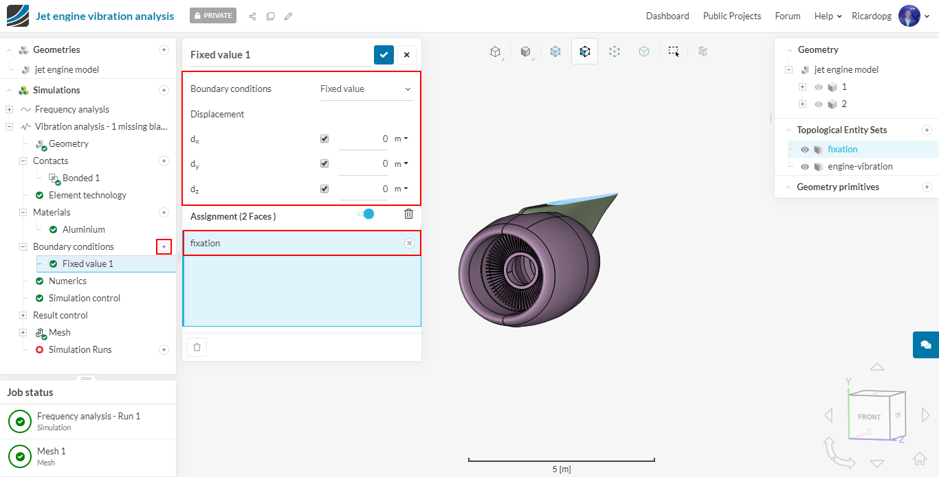
For the frequency analysis, the only boundary condition needed is the fixation of the wing. Click on the + sign next to Boundary conditions. From the drop down menu, choose Fixed value. The displacement in all directions will be 0. Assign it to the fixation topological entity set. You can rename this boundary condition fixation:
In Simulation control, make sure that Eigenfrequency Scope is set to First modes and that 20 modes will be analyzed:

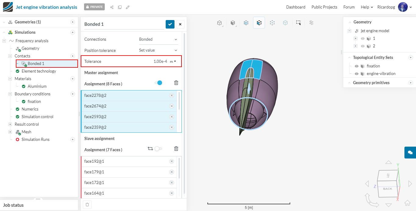
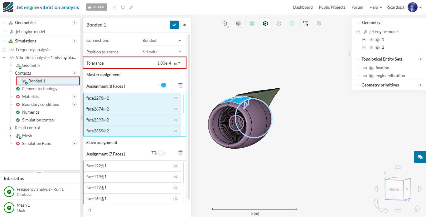
Before starting the simulation, expand Contacts in the simulation tree. Click on Bonded 1 and lower the Tolerance to 1e-4.
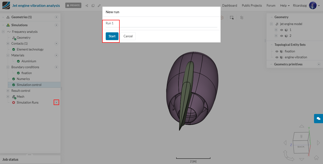
Now we can start our simulation. Go to Simulation Runs and click Start.
After the simulation finishes running, navigate to Plots to inspect the Eigenmode versus Eigenfrequency (Hz) plot:
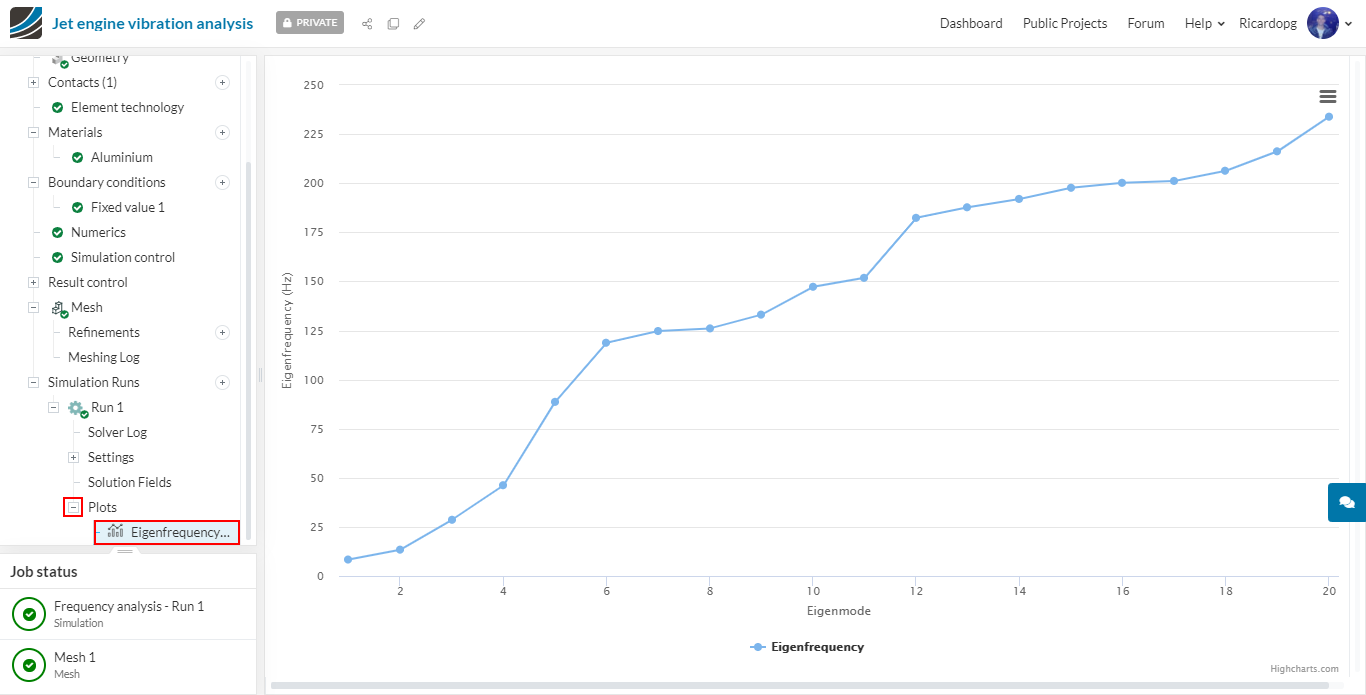
Jet engines usually run between 3000 and 6000 RPM (50 to 100 Hz). A total of 5 modes have eigenfrequencies under 100 Hz. 5 modes have their frequencies between 100 and 150 Hz.
Create further configurations
Configuration 2
Based on the frequency analysis result, we’re going to perform a series of harmonic analysis. Configuration 2 will simulate one missing blade. To start, create a new simulation, this time a Harmonic analysis:
To make the simulations easily distinguishable, rename this simulation Vibration analysis - 1 missing blade.
In Contacts, set Tolerance to 1e-4:
Materials will be Aluminium, just like the previous simulation. Assign it to volumes 1 and 2:
Now, in Boundary conditions, the first one will be a Fixed value, with 0 displacement in all directions. It will be assigned to the fixation topological entity set:
The applied force load due to the missing blades is estimated considering the following formulaton:
F=m*Δx*4π^2*f^2
Where:
- m is the mass of a missing blade. Considering a blade made of titanium (density equivalent to 4500 kg/m³), the mass of a blade will be roughly 7.65 kg.
- Δx is the distance of the dislocated center of mass, which is found out to be 5e-3 m;
To apply this condition, we will create a Force boundary condition. Rename the newly created BC to Jet engine load - Fy. Then follow the steps below:
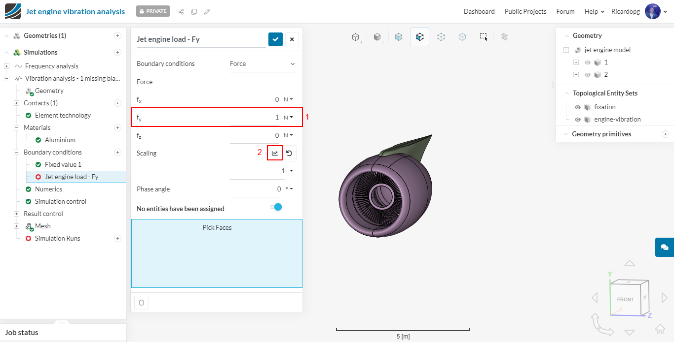
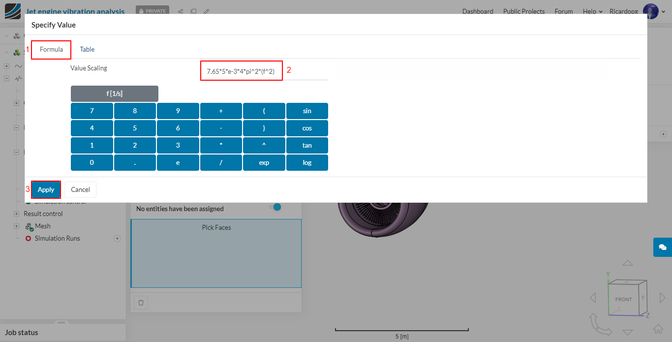
And input the following formula: 7.65*5*e-3*4*pi^2*(f^2)
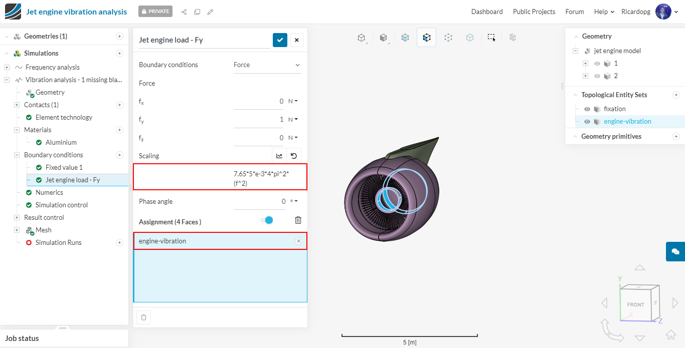
Lastly, assign this boundary condition to the engine-vibration topological entity set:
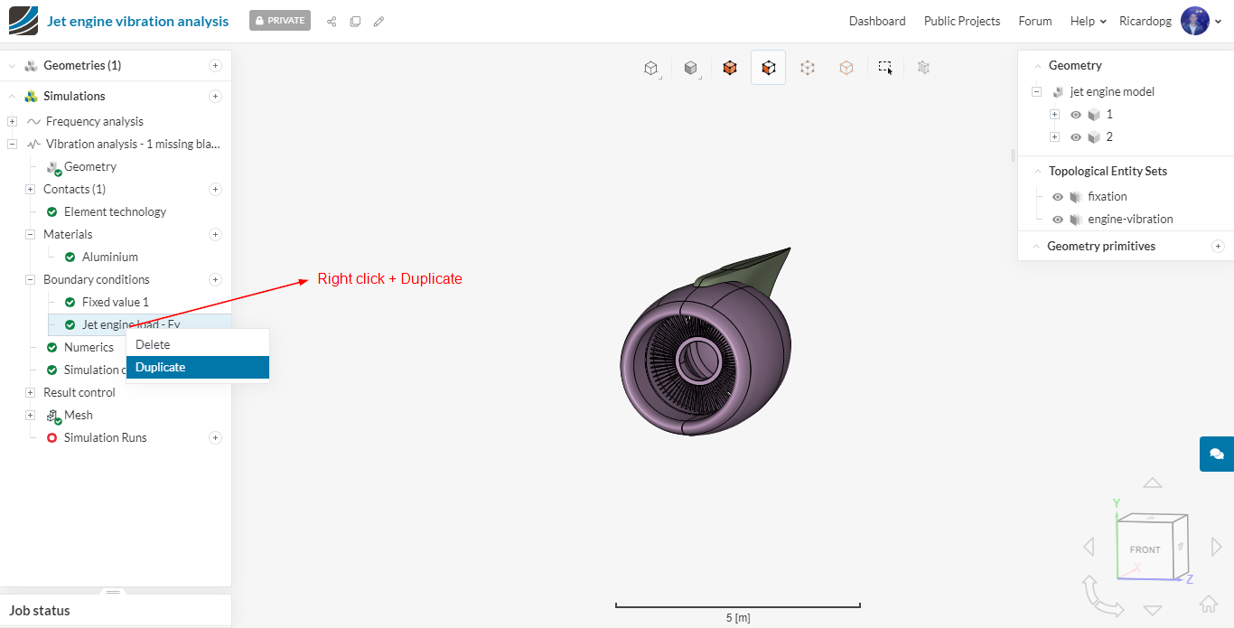
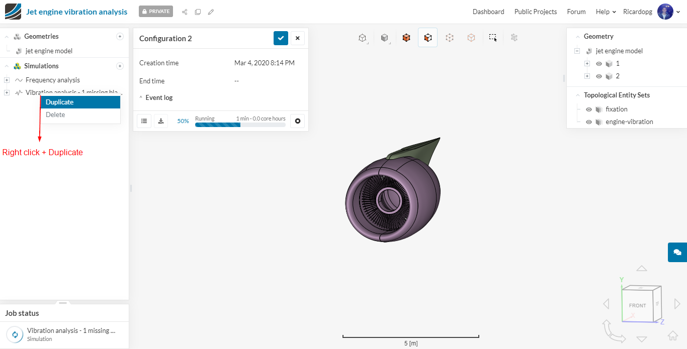
We will now make a similar boundary condition, but this time for the z direction. To do so, right click on the Jet engine load - Fy boundary condition and Duplicate it:
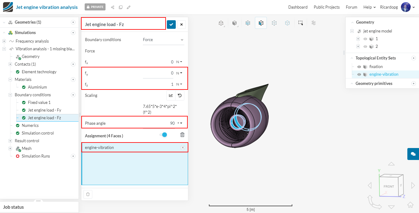
Rename this boundary condition Jet engine load - Fz. Change fy to 0 and fz to z. Also give a value of 90 to Phase angle:
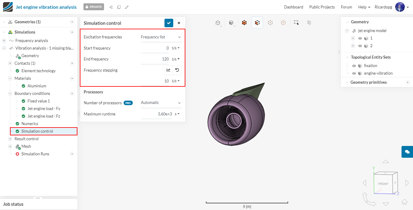
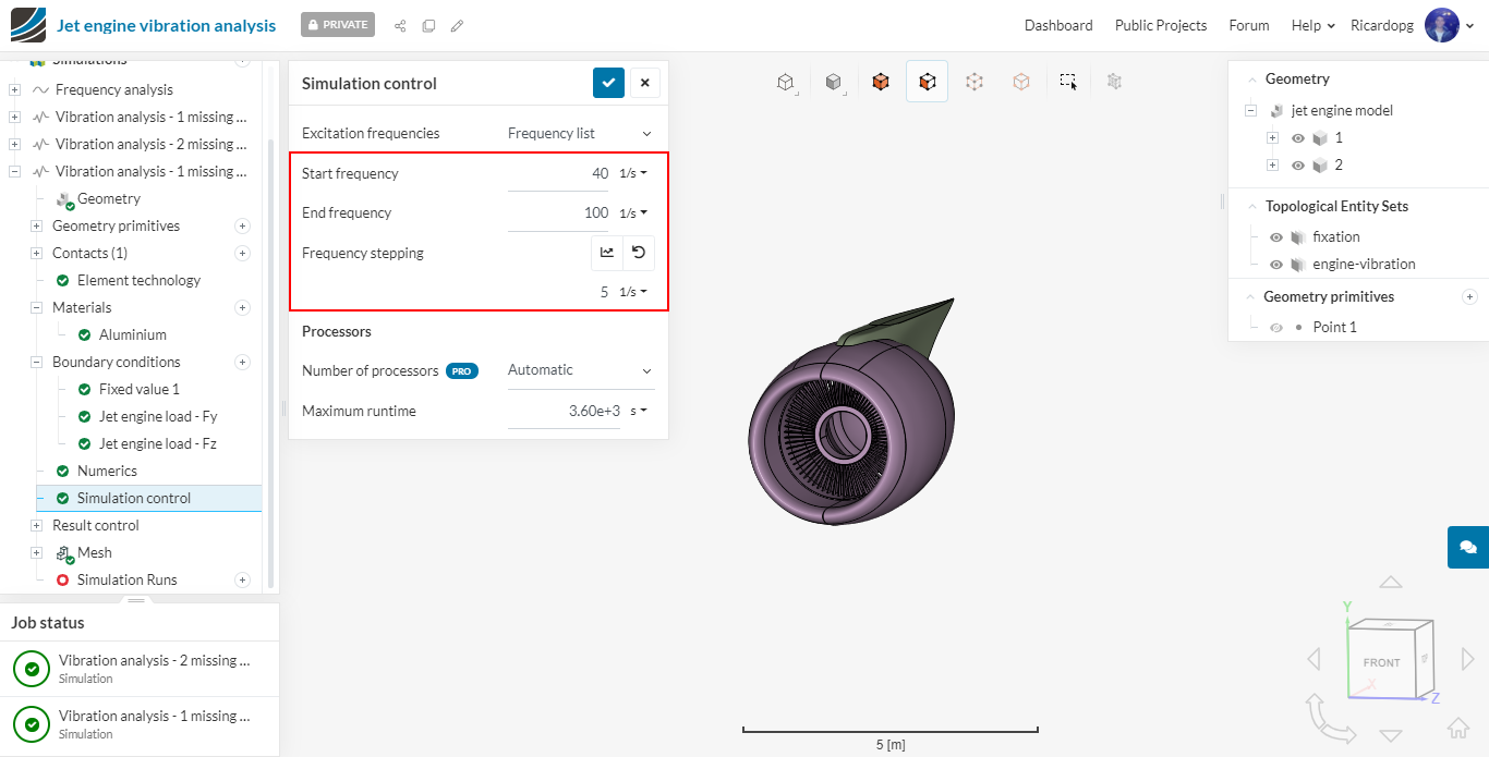
In Simulation control, change Excitation frequencies to Frequency list. Keeping in mind that engines usually run between 50 and 100 Hz, we will go from 0 to 120 Hz with steps of 10 Hz:
Expand Result control in the simulation tree. To save some computing time, we will delete some controls that are not of our interest. Please delete cauchy and von Mises stresses, aswell as total strain.
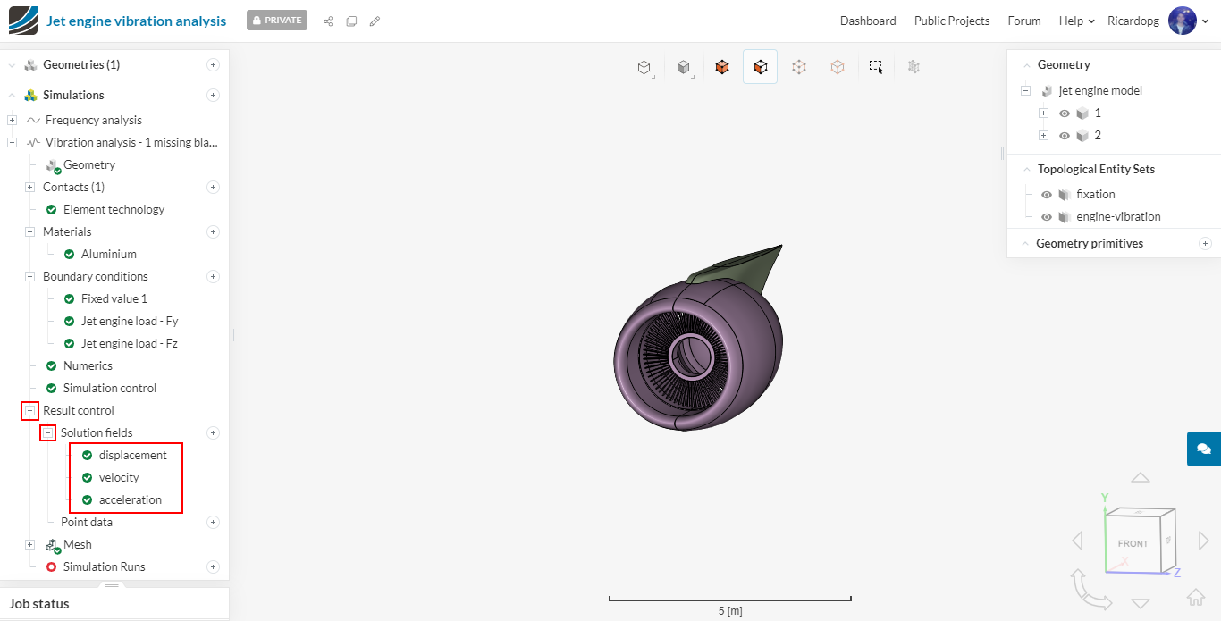
Next, we will create extra result controls under Point data. Rename the first one to Dx. It will be a Displacement control in the X direction. Change Complex number to Magnitude and phase:
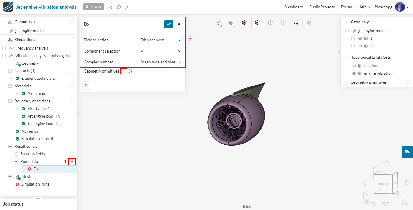
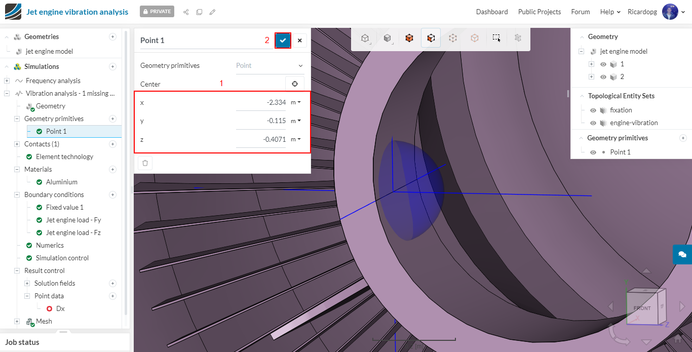
After clicking on the + button next to Geometry primitives, we will create one point where the displacement will be assessed. Give the following coordinates (x, y, z) for your point: -2.333779, -0.115045, -0.407097.
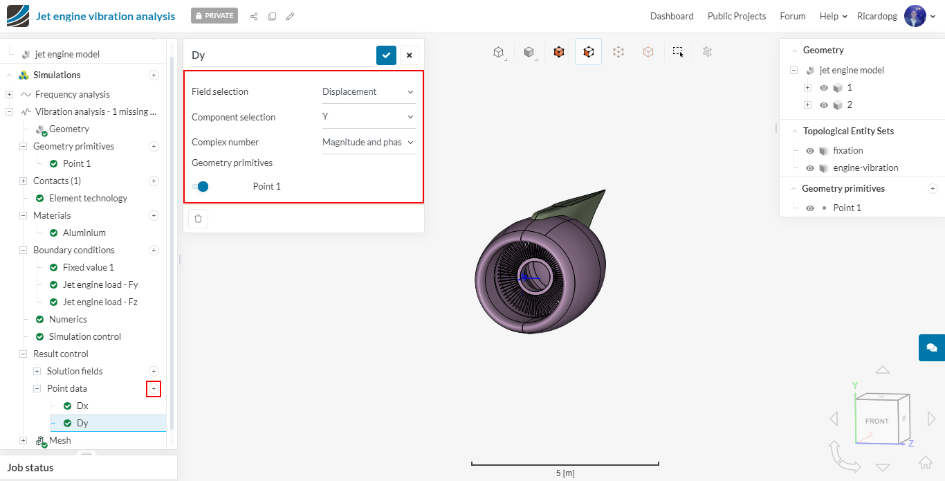
Similarly, create two extra controls for the Y and Z directions. The same point can be used.

That’s it for configuration 2. You can proceed to running the simulation.
Configuration 3
The first step is to duplicate the vibration analysis that was just set up. Rename is to ** Vibration analysis - 2 missing blades**
In Boundary conditions, change both load formulas to 15.3*8.42*e-3*4*pi^2*f^2.
You can proceed to creating a new Simulation Run for configuration 3.
Configuration 4
For configuration 4, duplicate the simulation named Vibration analysis - 1 missing blade.
Based on the results from ‘Configuration 2’, it is evident that the peak of displacement is between 40 to 100 Hz. Therefore, we will now redefine our frequency range and rerun the case in order to get the exact frequency where the peak displacement is taking place.
Go to Simulation Control and change Start frequency to 40 Hz, End frequency to 100 Hz and Frequency stepping to 5.
After changing these values, please create a simulation run for configuration 4.
Configuration 5
Duplicate the simulation named Vibration analysis - 2 missing blades. Change the start and end frequency values, aswell as frequency stepping to those from configuration 4. Then please run the last simulation.
Post-processing
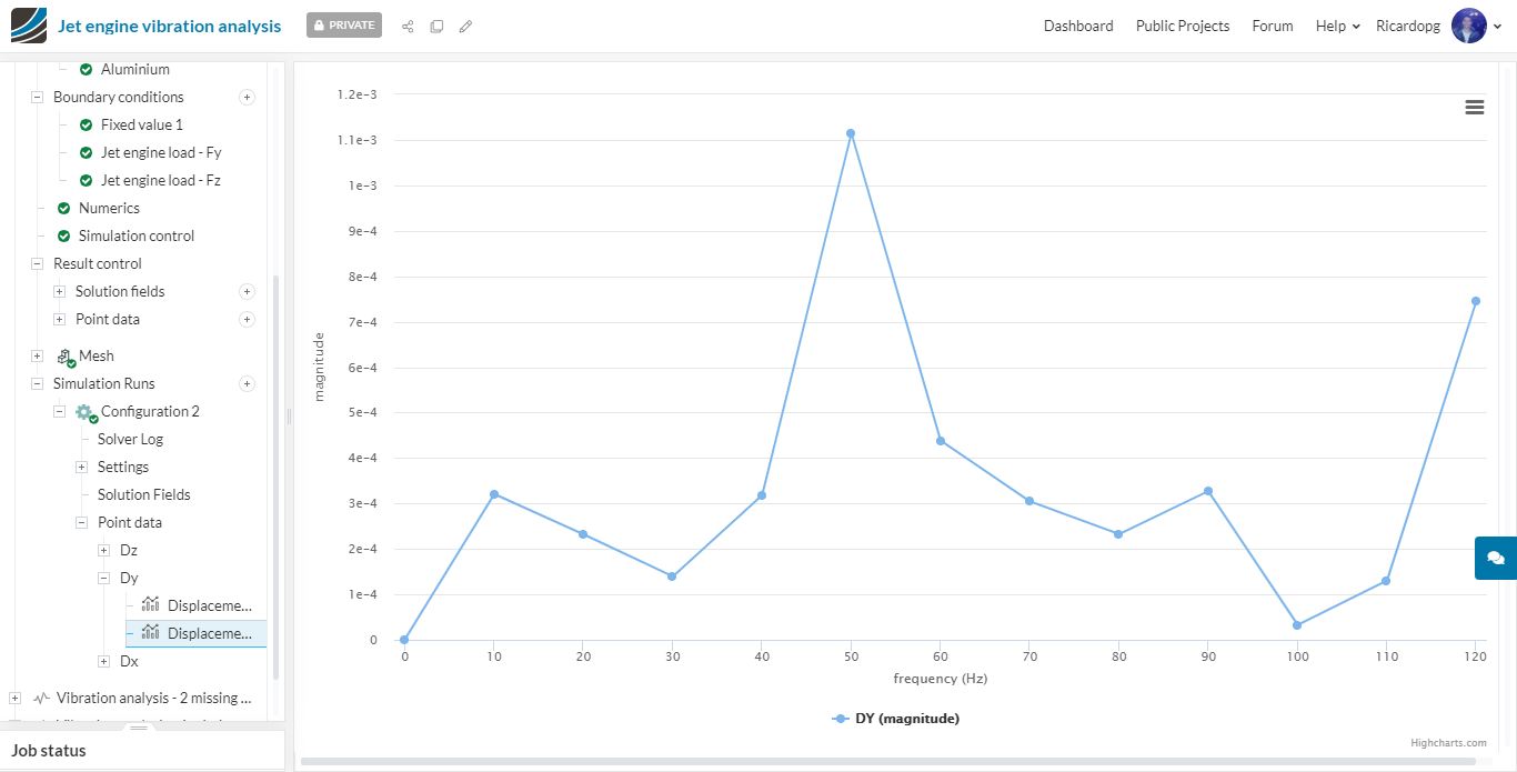
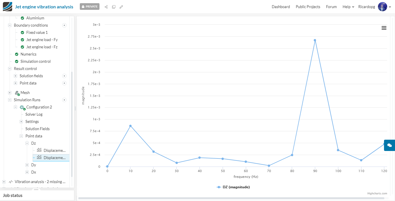
The vibration was studied for the missing blade vibration load within the frequency range of 0 to 120 Hz (0 to 7200 rpm). The most important result in this case is the displacement plot in y and z direction. Below are the displacement plots of Configuration 2 and Configuration 3:
Configuration 2 - Dy:
Configuration 2- Dz:
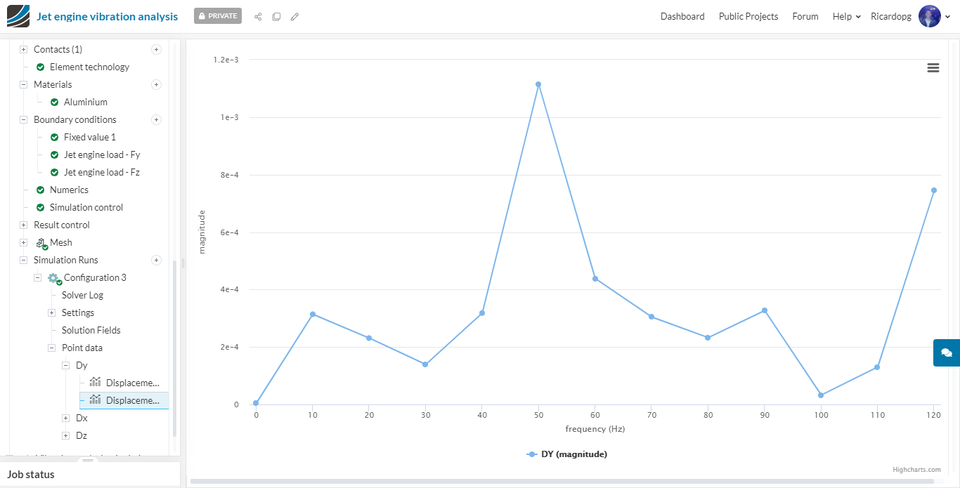
Configuration 3 - Dy:
Configuration 3 - Dz:
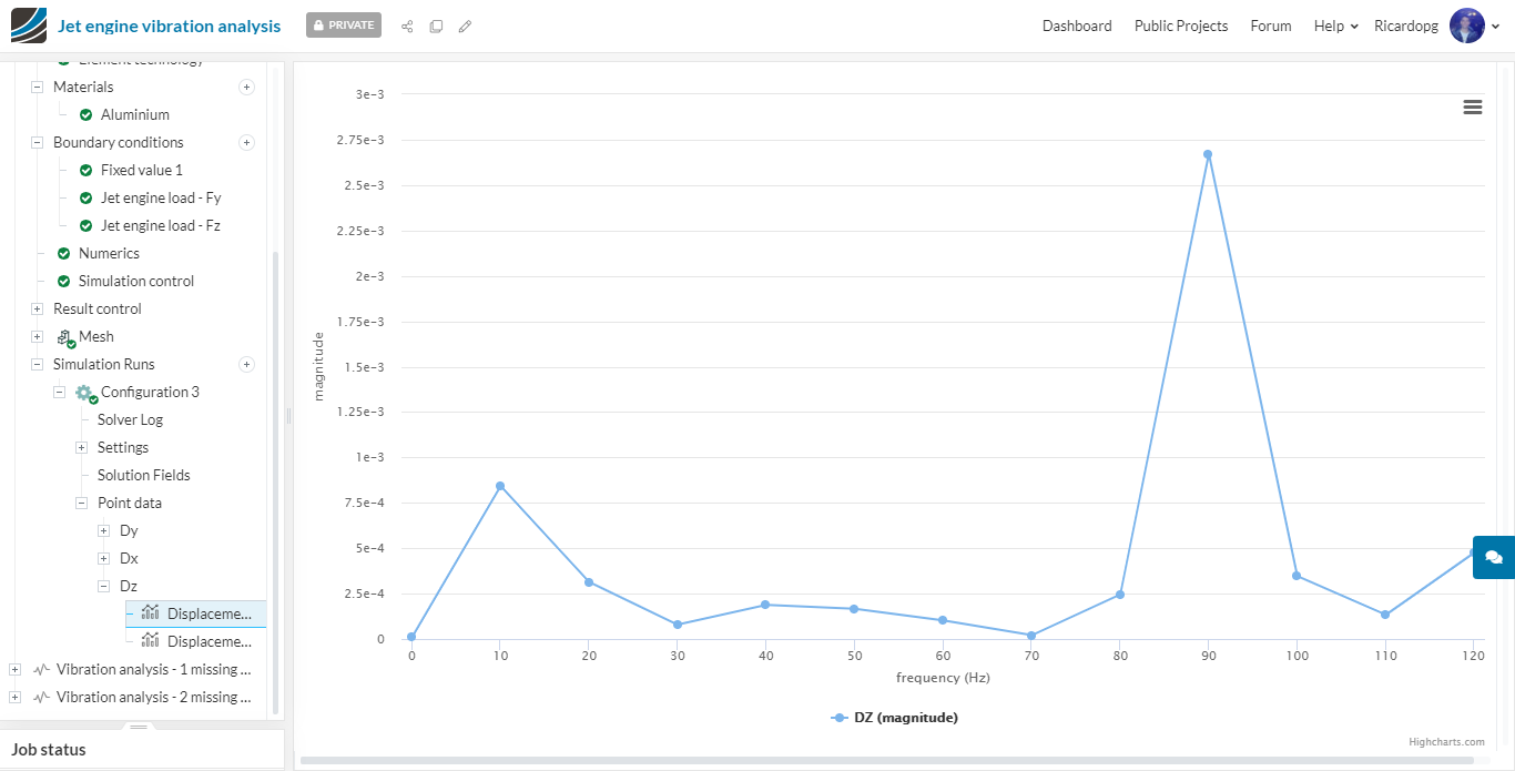
Despite the extra blade that was missing, the displacements observed in configurations 2 and 3 are almost the same.
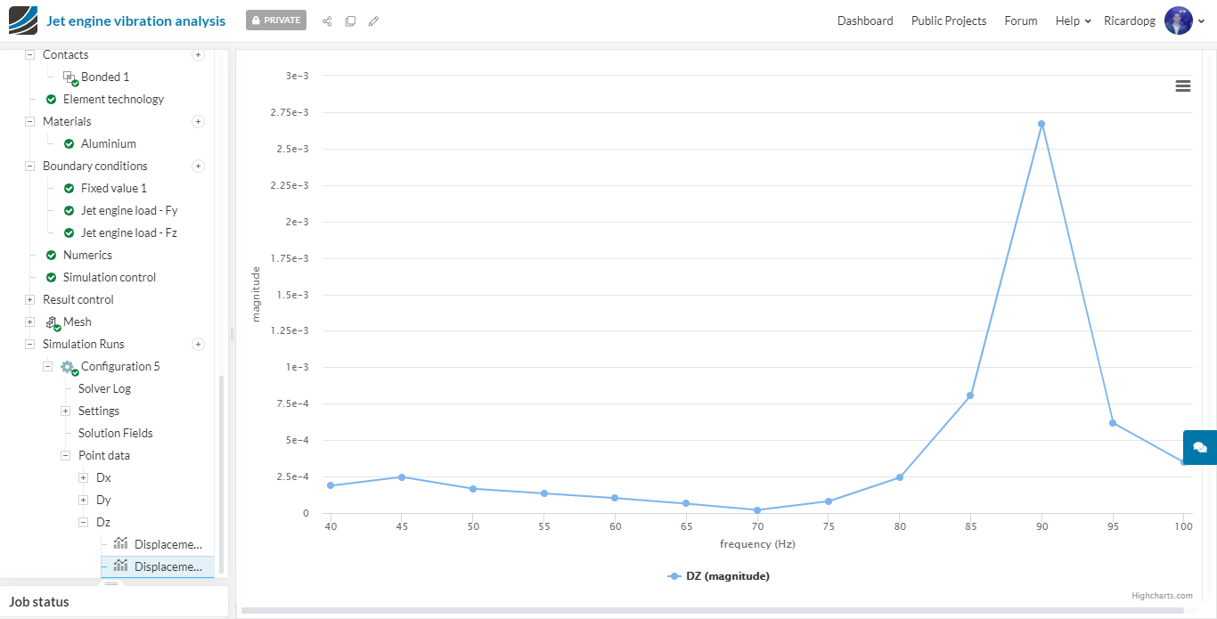
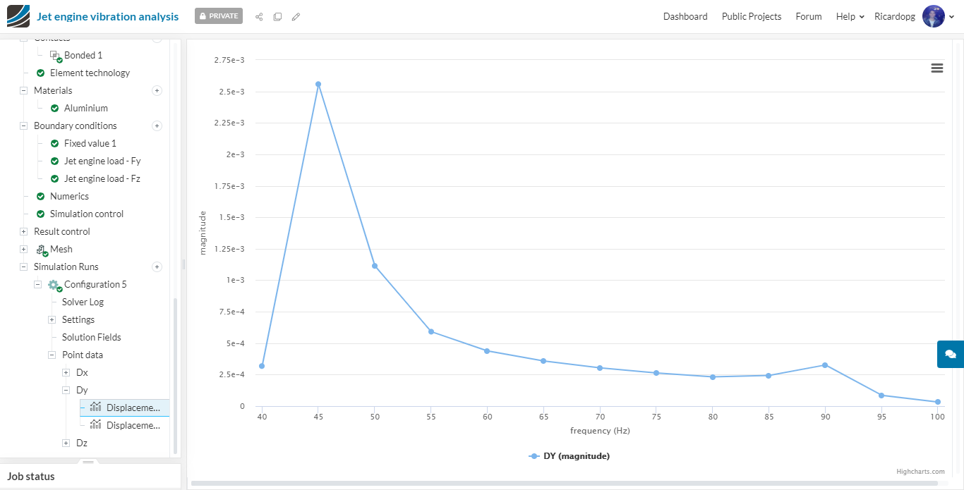
Now taking a closer look at Configurations 4 and 5, in case engine blades are missing, the maximum vibration in the cowling will occur at the frequencies of 45 and 90 Hz:
Configuration 5 - Dy
Configuration 5 - Dz