Recording
Aerospace Workshop II feat. EUROAVIA (Session 2) ― Structural Analysis of a Jet Engine Bracket
Exercise
The part we are simulating in this project is an aircraft engine bearing bracket. The function of this bracket is to support the weight of the cowling during engine service whereas it plays no active role during the operation of the engine.
Three of the models are used in this homework provided by GrabCAD users who were the winners of the GrabCAD ‘Airplane Bearing Bracket Challenge ’. The models are shown in the figure below with order of first, second and third as model_1, model_2 and model_3.
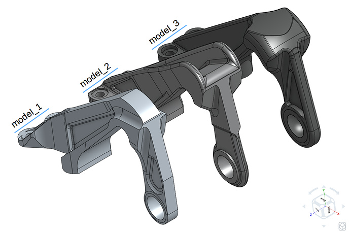
- 1st position: model_1 provided by Igor Nikolaychuk from GrabCAD . | Strength/Weight: ~99.76 kN/kg
- 2nd position: model_2 provided by Allar Õunsaar from GrabCAD . | Strength/Weight: ~96.40 kN/kg
- 3rd position: model_3 provided by Krisztián Haász from GrabCAD . | Strength/Weight: ~86.97 kN/kg
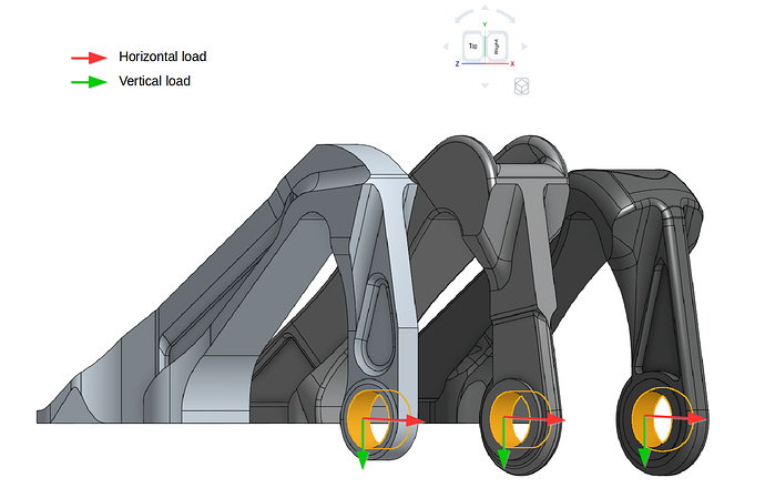
This exercise focuses on the the testing of these three models based on the similar horizontal and vertical load provided in the GrabCAD challenge . In addition to this, the models were further tested considering the nonlinear plastic material and also increasing both loads. The applied constraint and loading boundary conditions are shown below. Please note that separate simulations were created for both loading types.
The different combinations for performing the simulations are:
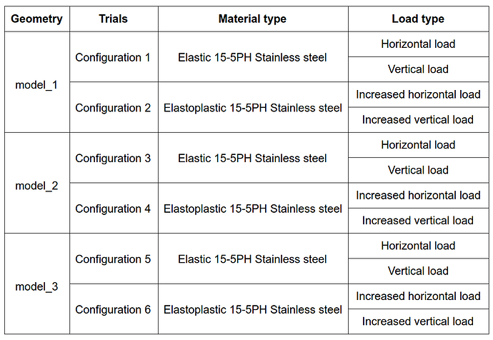
Please note that separate simulation needs to be set up for each configuration
Step-by-Step
Import the project by clicking the link below. (Crtl + Click to open in a new tab)
This step-by-step will focus on the set up of the first model. Configurations 3, 4, 5 and 6 follow the same procedure shown here.
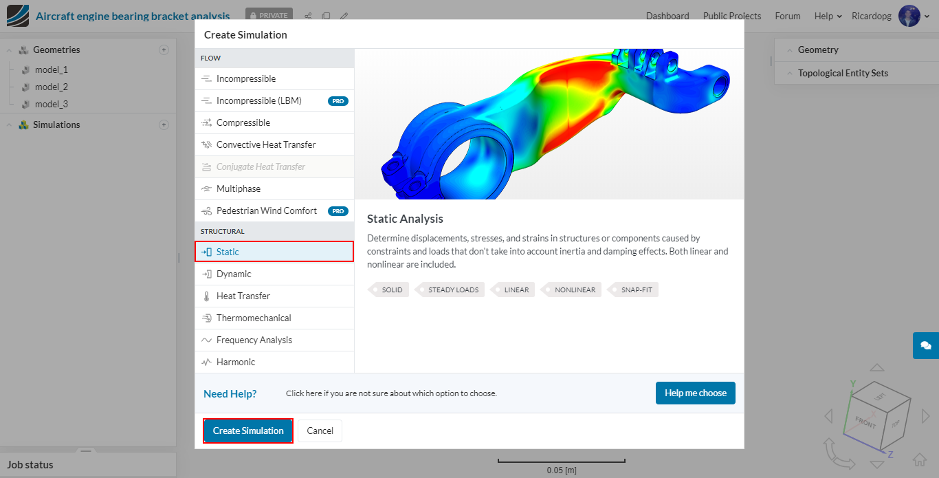
In the left-hand side panel, select model_1 and then click on Create a SImulation.

We will carry out a Static analysis.
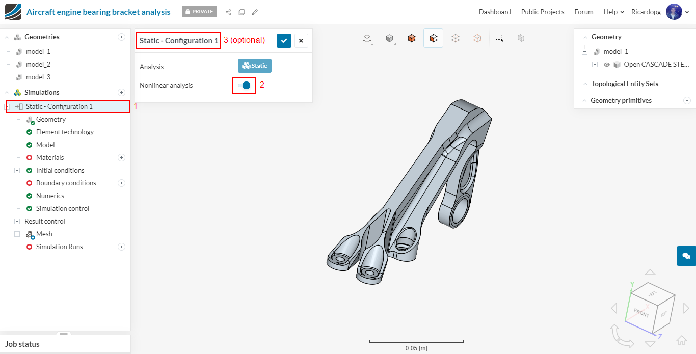
After creating the simulation, please enable Nonlinear analysis. To avoid confusion with the other set ups, you can rename this simulation to Static - Configuration 1.
Meshing
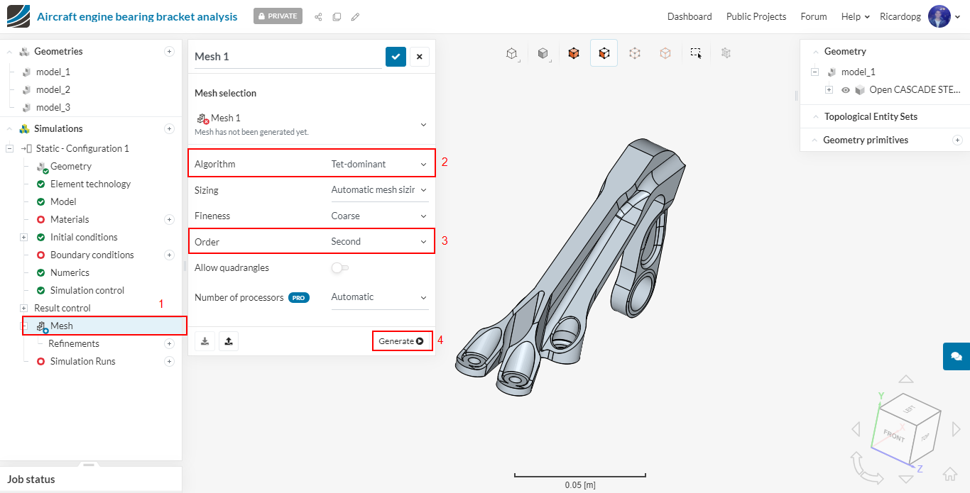
In the simulation tree (left-hand side panel), navigate to Mesh. Change the Algorithm to Tet-dominant. Make sure the Order of elements is Second. Fineness remains as Coarse.
After making these changes, go ahead and click on the Generate button to start the meshing operation. The number of processors used is automatically optimized by SimScale.
Settings for the meshing operation are the same for the other models.
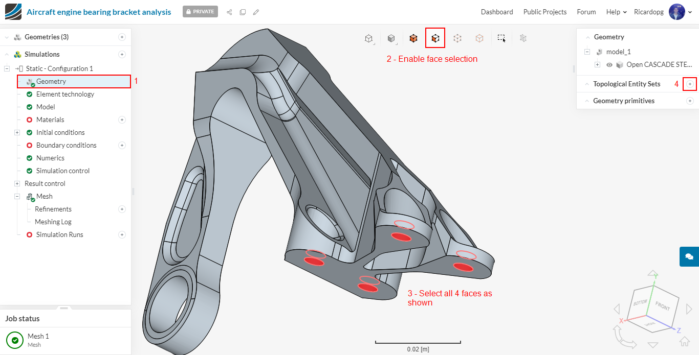
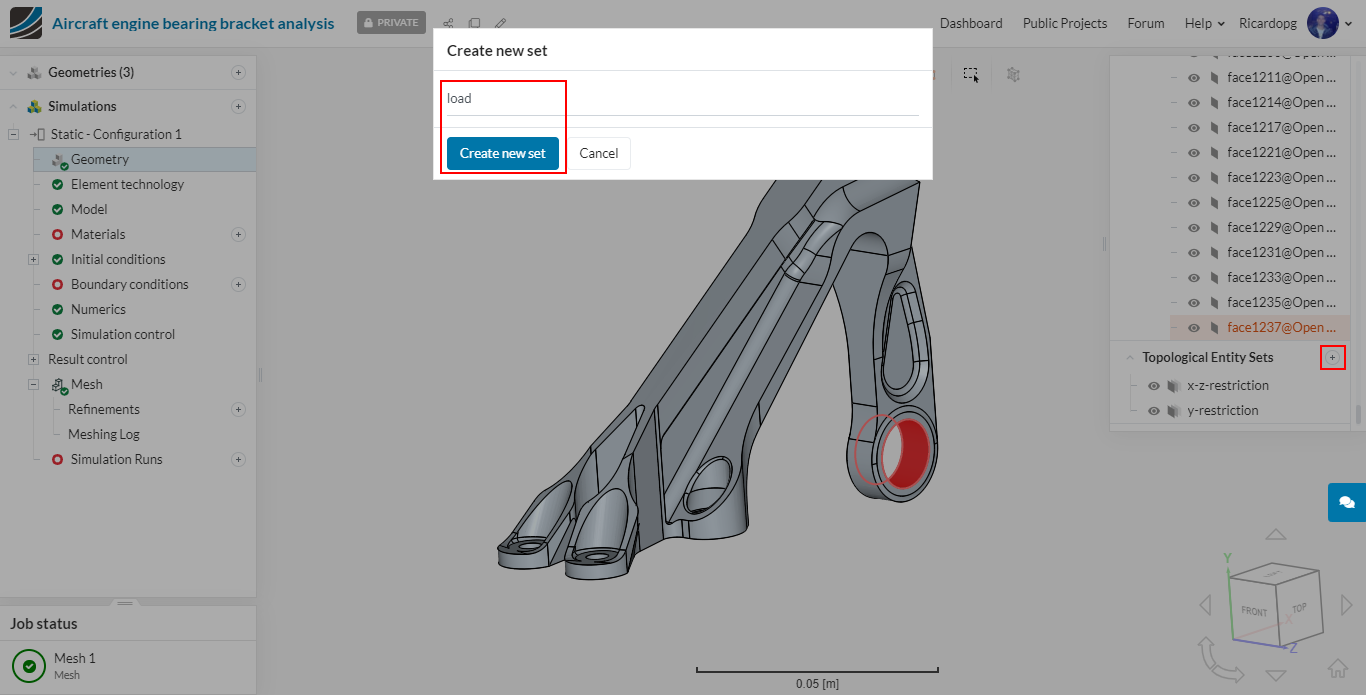
Topological Entity Sets
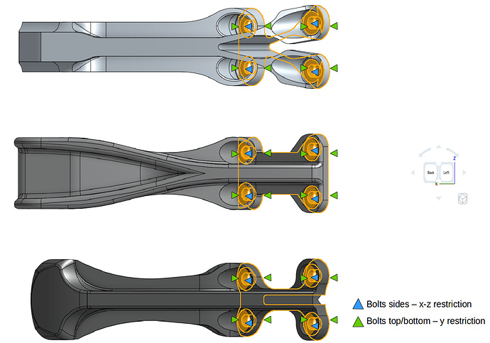
The figures below explain all the boundary and loading conditions from the parts. The Topological Entity Sets that will be created are based on these loading conditions.
We will create total of 3 topological entity sets as shown below:
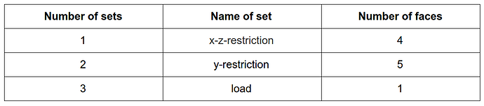
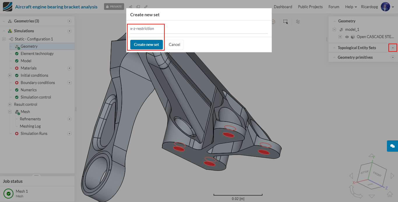
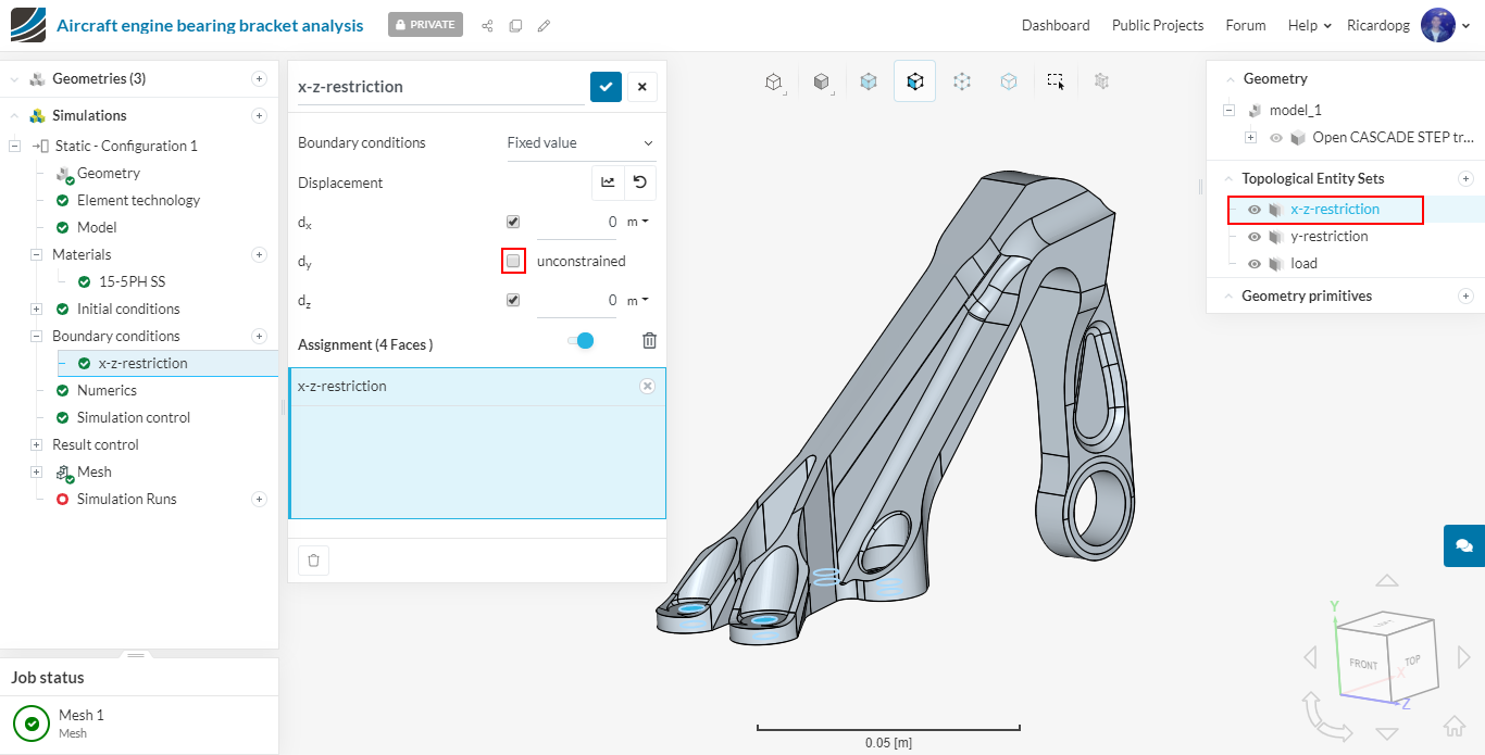
To create the x-z-restriction topological entity set, follow the steps below:
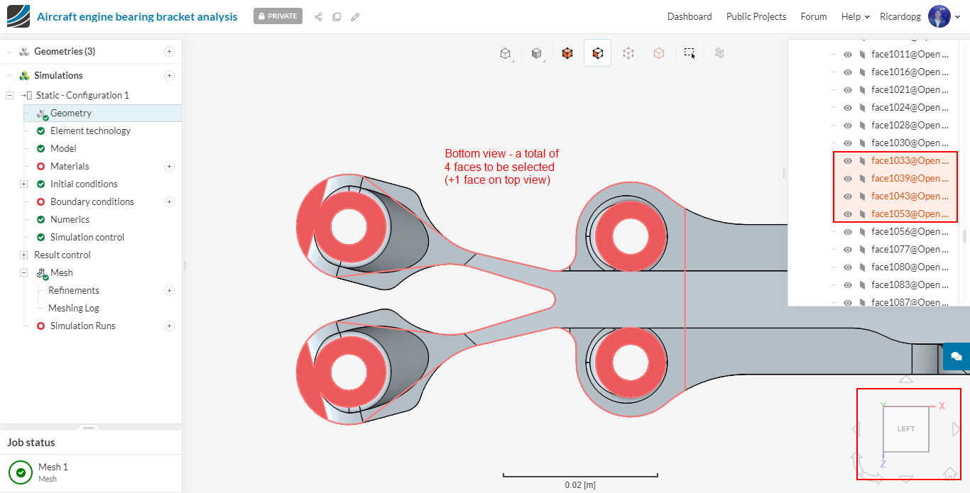
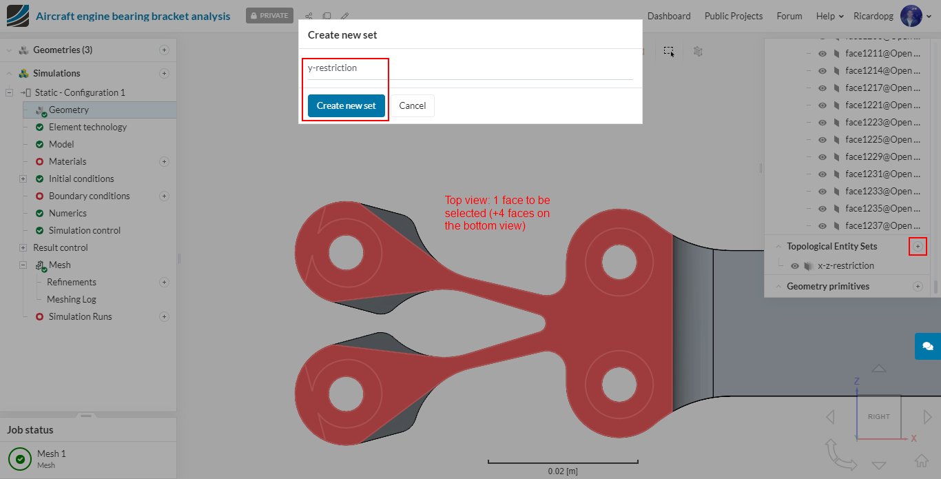
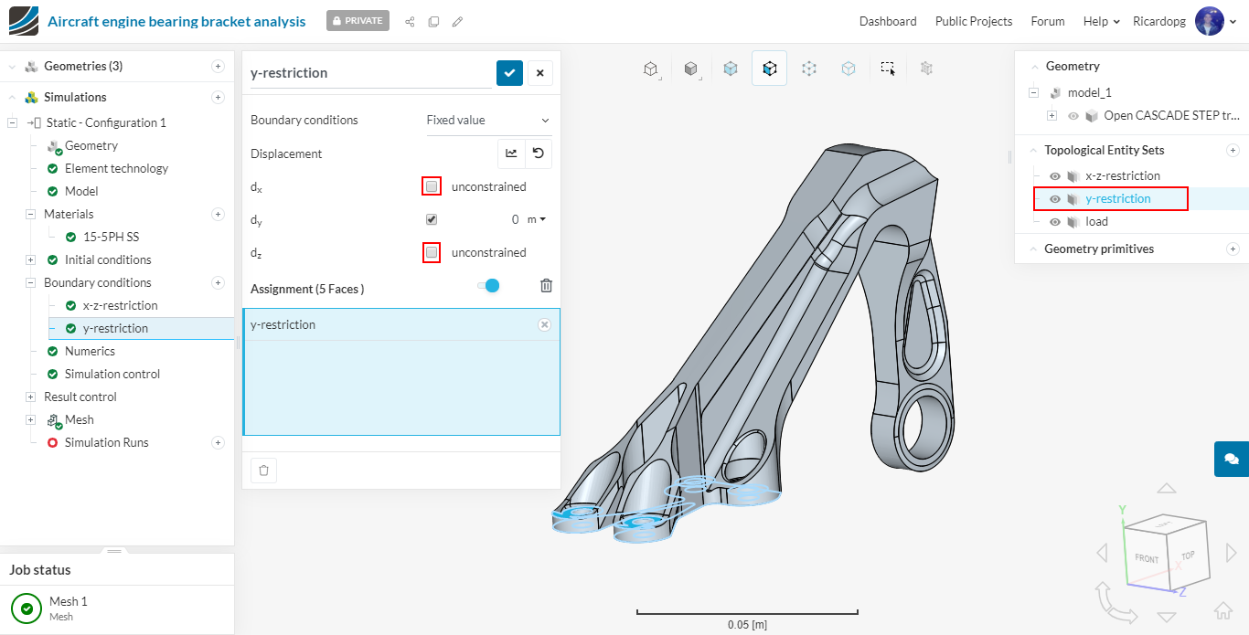
To create a y-restriction topological entity set, select the upper and lower face of the geometry on bolt fixation as shown in the figure below.
To create a load topological entity set, do as follows:
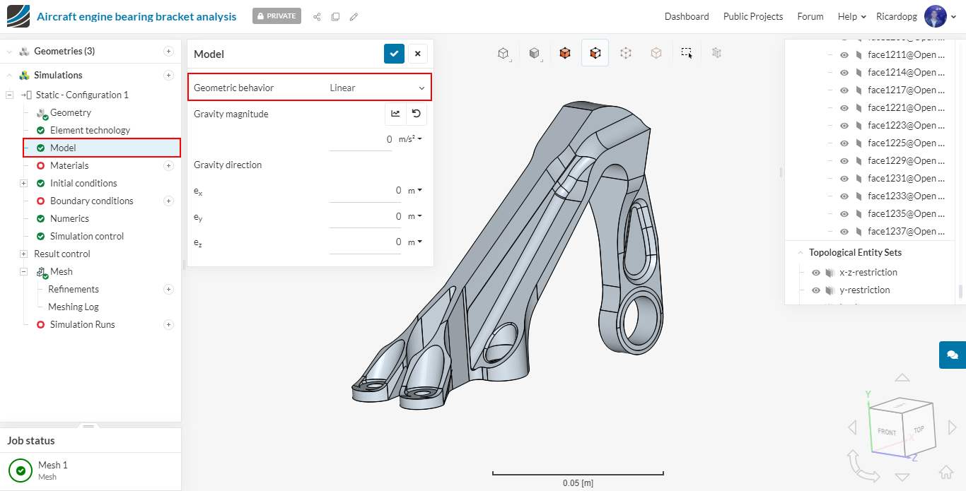
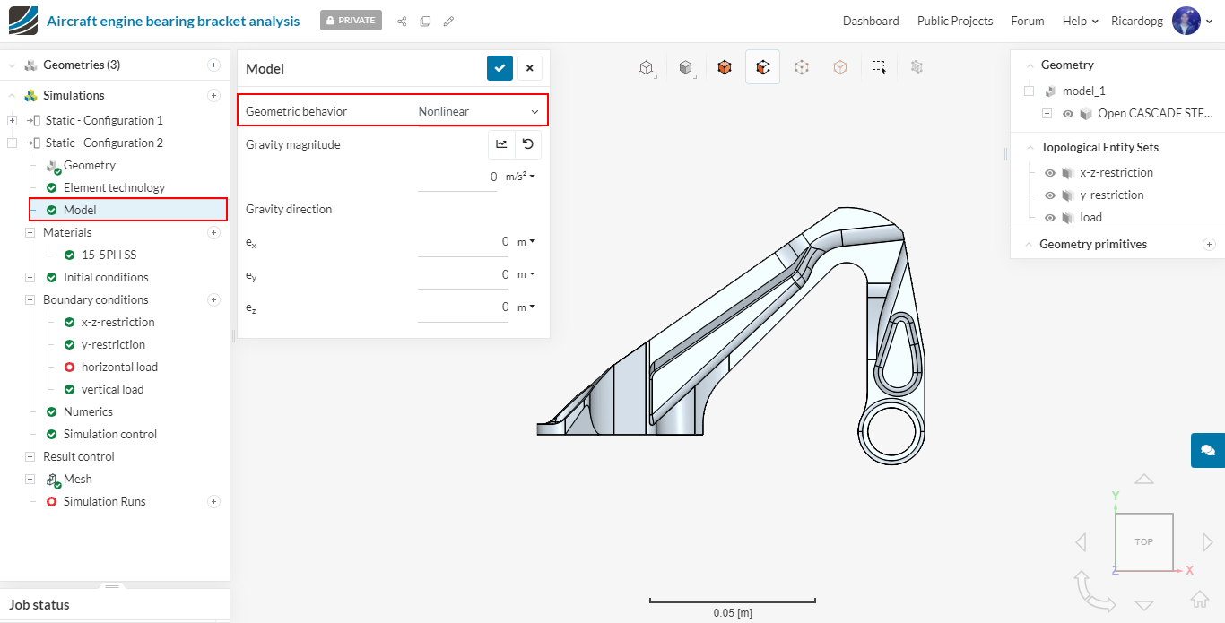
Now, in the simulation tree, please navigate to Model. Due to small load conditions, turn off the geometric nonlinearity by setting Geometric behavior to Linear.
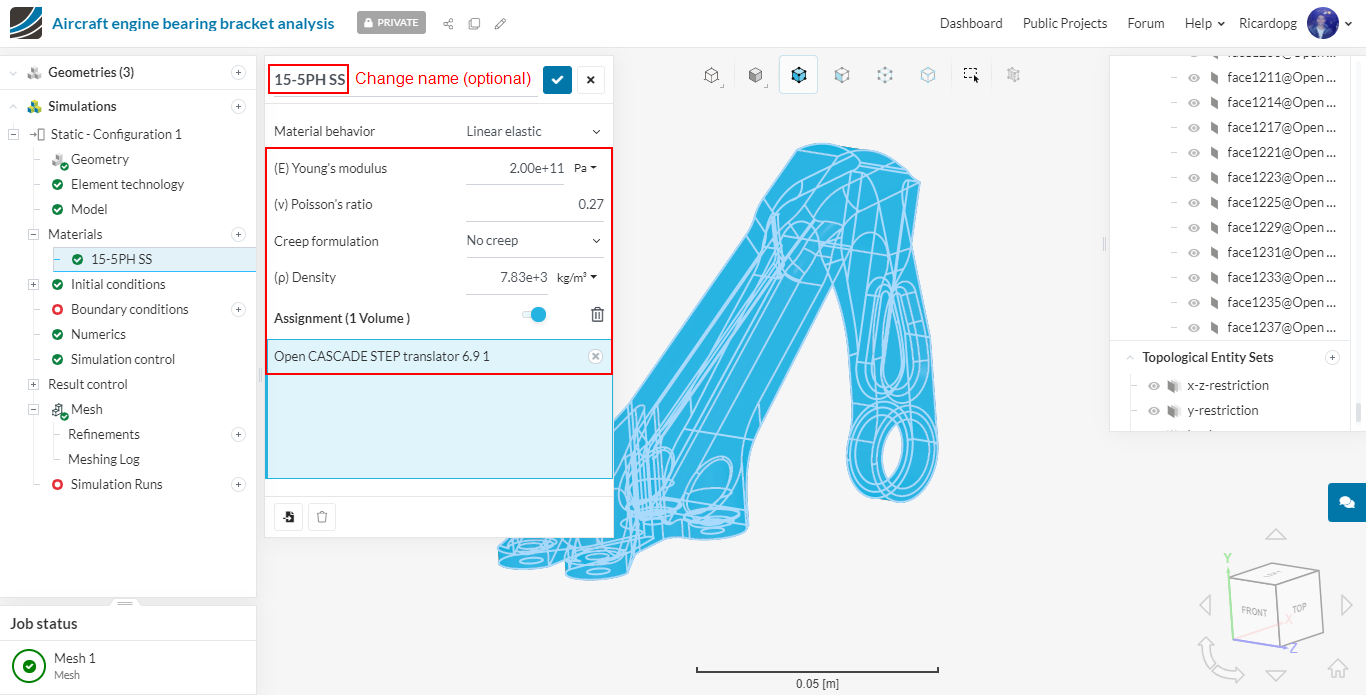
It’s time to assign a Material to our part. For Configuration 1 we have to only define an elastic material for our bearing bracket. The material we are going to use is 15-5PH Stainless steel, which is a fairly tough material with high yield strength of 1 GPa.
In the simulation tree, click on Materials, select Steel and click on Apply.

Rename newly created material to 15-5PH SS (optional). Change the (E) Young’s modulus, (ν) Poisson’s ratio and Density values to 200e9 , 0.27 and 7833, respectively, as shown in figure below.
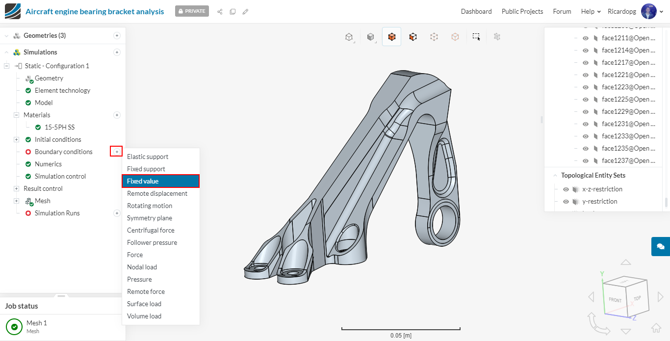
Boundary conditions
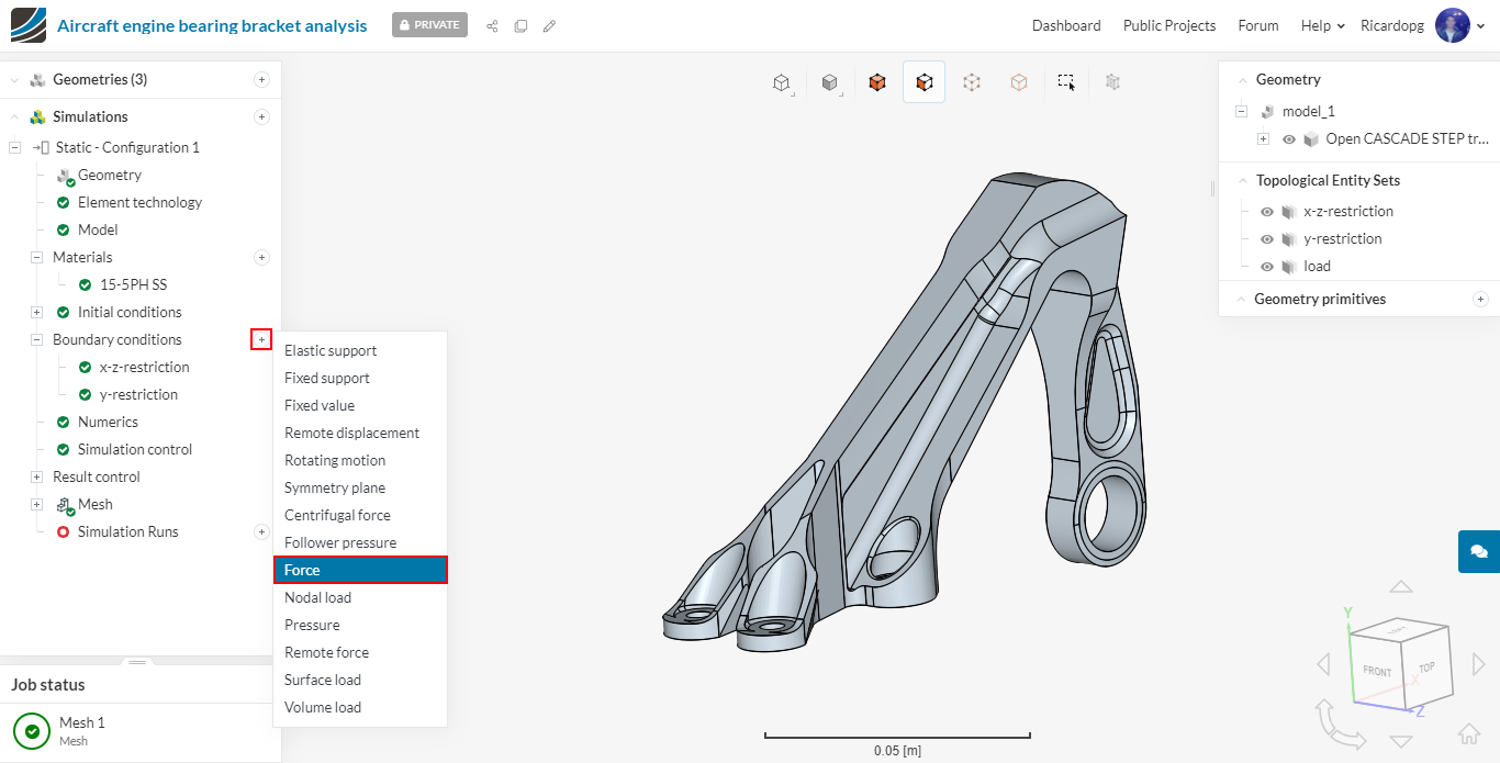
To create a new boundary condition, click on the + icon and select the desired type. We are going to use the previously created topological entity sets to help us.
The x-z-restriction boundary condition will be a Fixed value condition.
Uncheck dy displacement to make it unconstrained. Assign this boundary condition to the x-z-restriction topological entity set:
The y-restriction boundary condition will be a Fixed value condition. Uncheck dx and dz displacement to make them unconstrained. Assign this boundary condition to the y-restriction topological entity set:
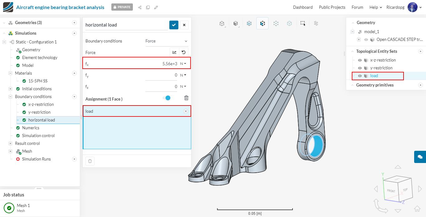
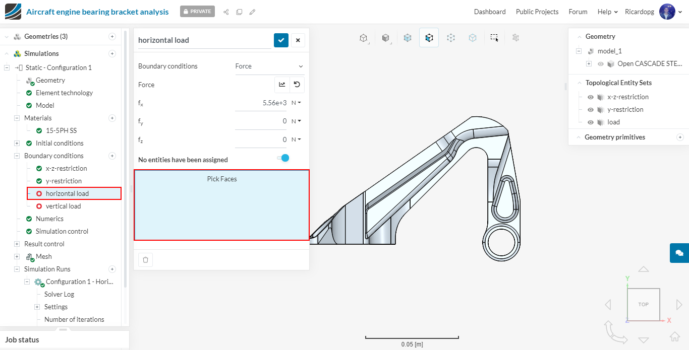
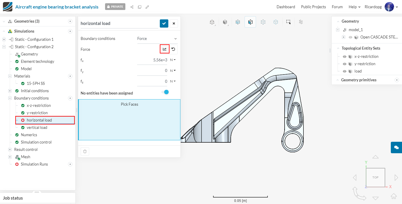
Next we will define our horizontal load boundary condition. This one will be a Force condition.
Give a value of 5560 N to fx and assign the boundary condition to the load topological entity set. Rename this boundary condition horizontal load (optional).
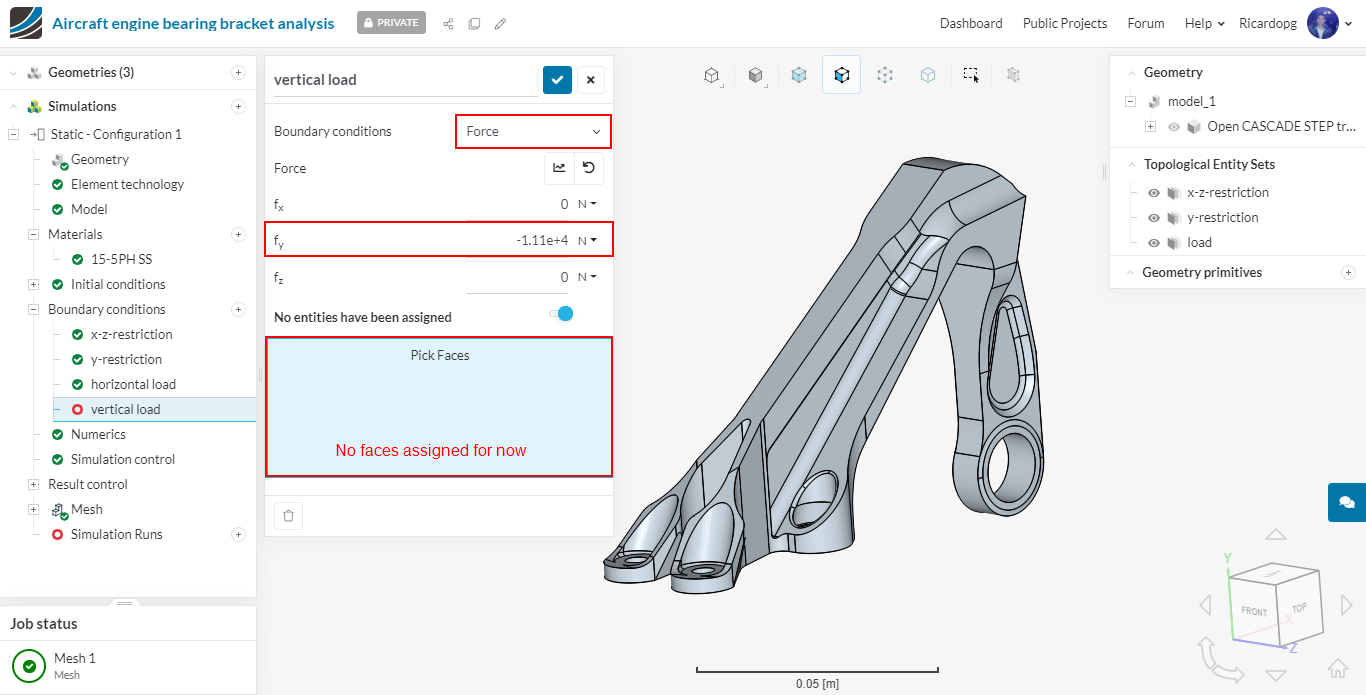
We will also create a boundary condition for the vertical load. This boundary condition won’t be used for configuration 1, but will be used for some of the other configurations. Follow the same procedure as above, This time assign a value of -11120 N to fy. Don’t assign this boundary condition to any faces.
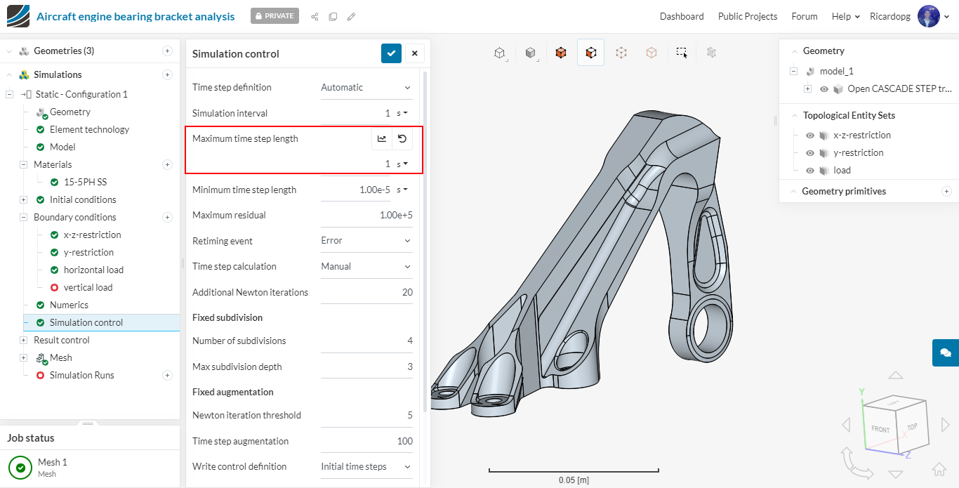
Simulation control
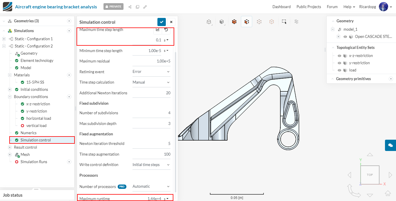
Navigate to Simulation control. Change Maximum time step length to 1 second (as this is a linear static analysis therefore one analysis step would be enough) , The number of cores used is once again automatically chosen.
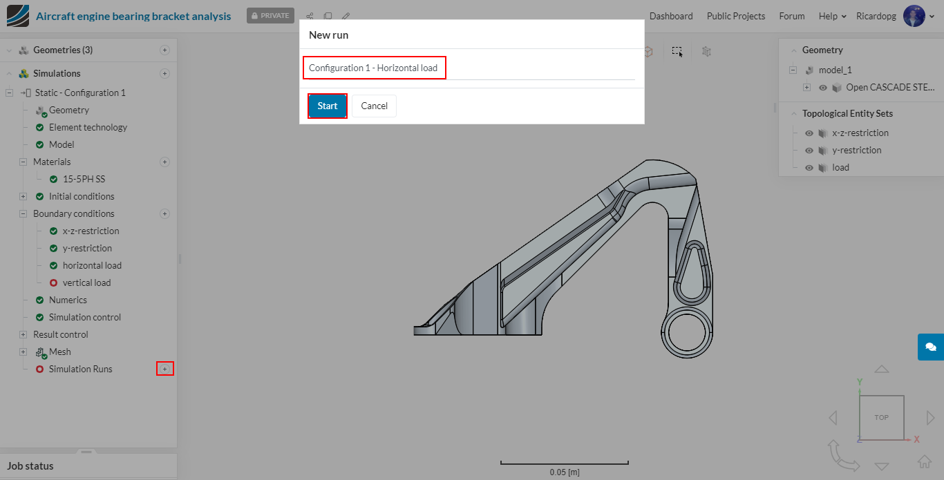
The setup is ready. Proceed to Simulation Runs, name your run appropriately (e.g. Configuration 1 - Horizontal load) and hit Start (ignore the warnings that pop up).
This simulation takes less than 10 minutes to complete.
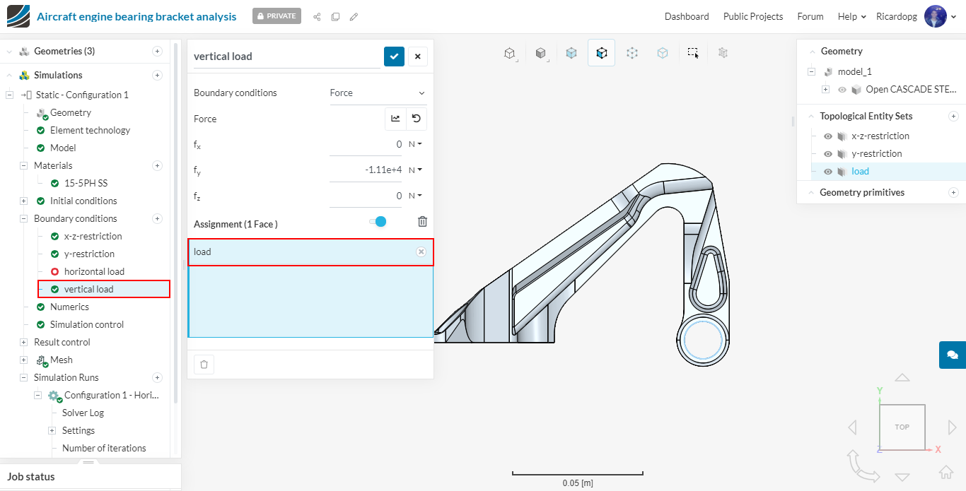
Vertical load case:
For the vertical load case of configuration 1, head back to Boundary conditions. First click on the horizontal load boundary condition and leave it with no faces assigned:
And assign the vertical load boundary condition to the load topological entity set:
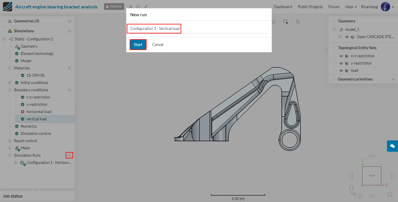
Head over to Simulation Runs and Start another run. Following the same pattern, name it Configuration 1 - Vertical load (ignore the warnings that pop up).
Create further configurations
Configuration 2
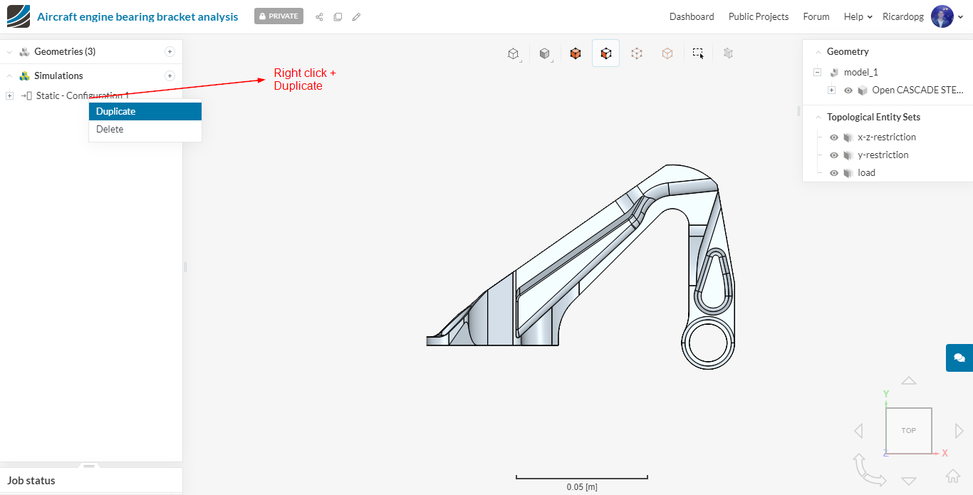
Once you have started all the runs with the first configuration setup, go ahead and make a duplicate of this simulation in order to perform the simulation with different material type for hip joint.
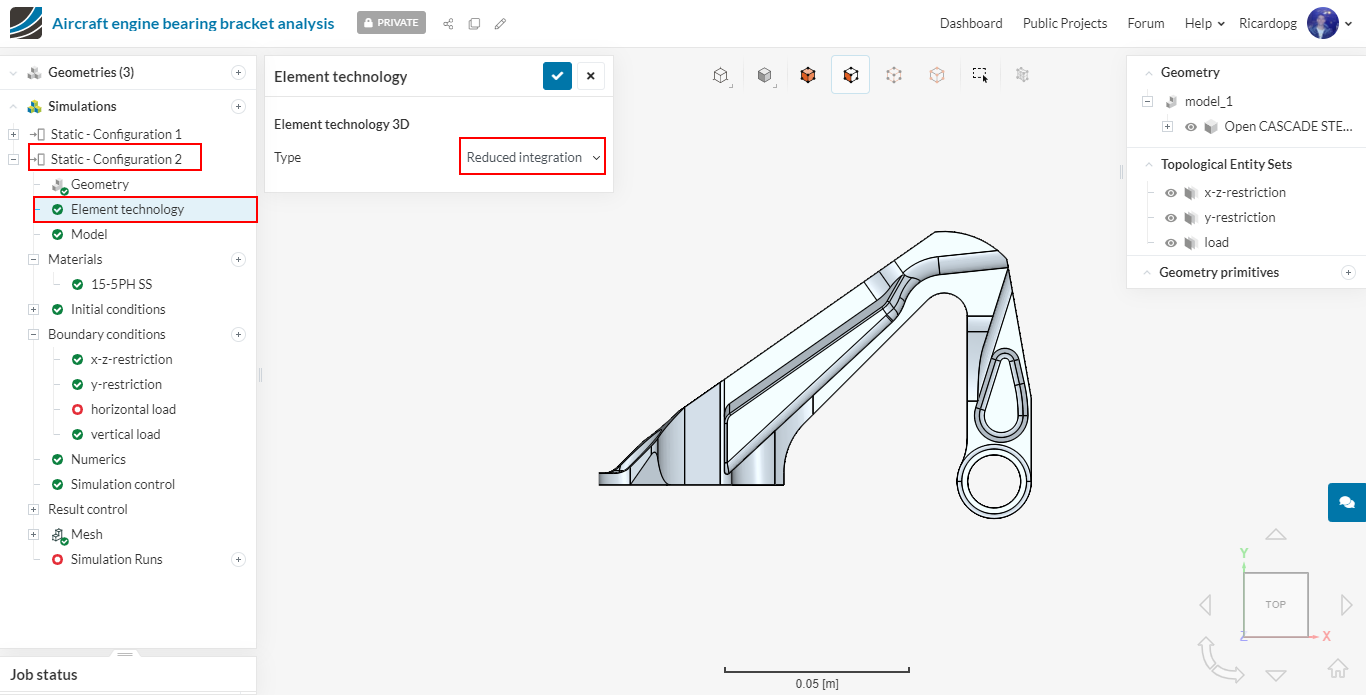
In the new simulation tree, click on Element technology. Since we are going to deal with a plastic material using second order elements, it’s always recommended to use reduced integration element technology to get the more realistic results.
In Model, we will now turn back to the geometric nonlinearity, due to the large load conditions. So please switch Geometric behavior to Nonlinear.
Materials: Now we will define a plastic material for which we have to first create a .csv file with our plastic material data. The stress strain data in this .csv file will start from yield point of 15-5PH stainless steel. Just copy the values given below, create a new ‘Notepad’ (or any notepad application) file on your computer and paste them there. Save the file by first changing the file types to all types. Then give it some reasonable name e.g. 15-5PH-SS-stress-strain.csv in this case and click ‘Save’. (material data is taken from [1])
0.0050,1.0000E+09
0.0077,1.0696E+09
0.0094,1.1154E+09
0.0115,1.1482E+09
0.0150,1.1591E+09
0.0181,1.1700E+09
0.0207,1.1896E+09
0.0242,1.2158E+09
0.0297,1.2464E+09
0.0344,1.2813E+09
0.0412,1.3206E+09
0.0488,1.3643E+09
0.0570,1.4057E+09
0.0663,1.4450E+09
0.0755,1.4690E+09
0.0849,1.4756E+09
0.0962,1.4603E+09
0.1049,1.4254E+09
0.1144,1.3774E+09
0.1226,1.3315E+09
0.1301,1.2791E+09
0.1367,1.2289E+09
0.1431,1.1787E+09
0.1495,1.1154E+09
After creating the file, go to 15-5PH SS under Materials and change Material behavior to Plastic. Change (E) Young’s modulus and Poisson’s ratio to 2e11 and 0.27 respectively.
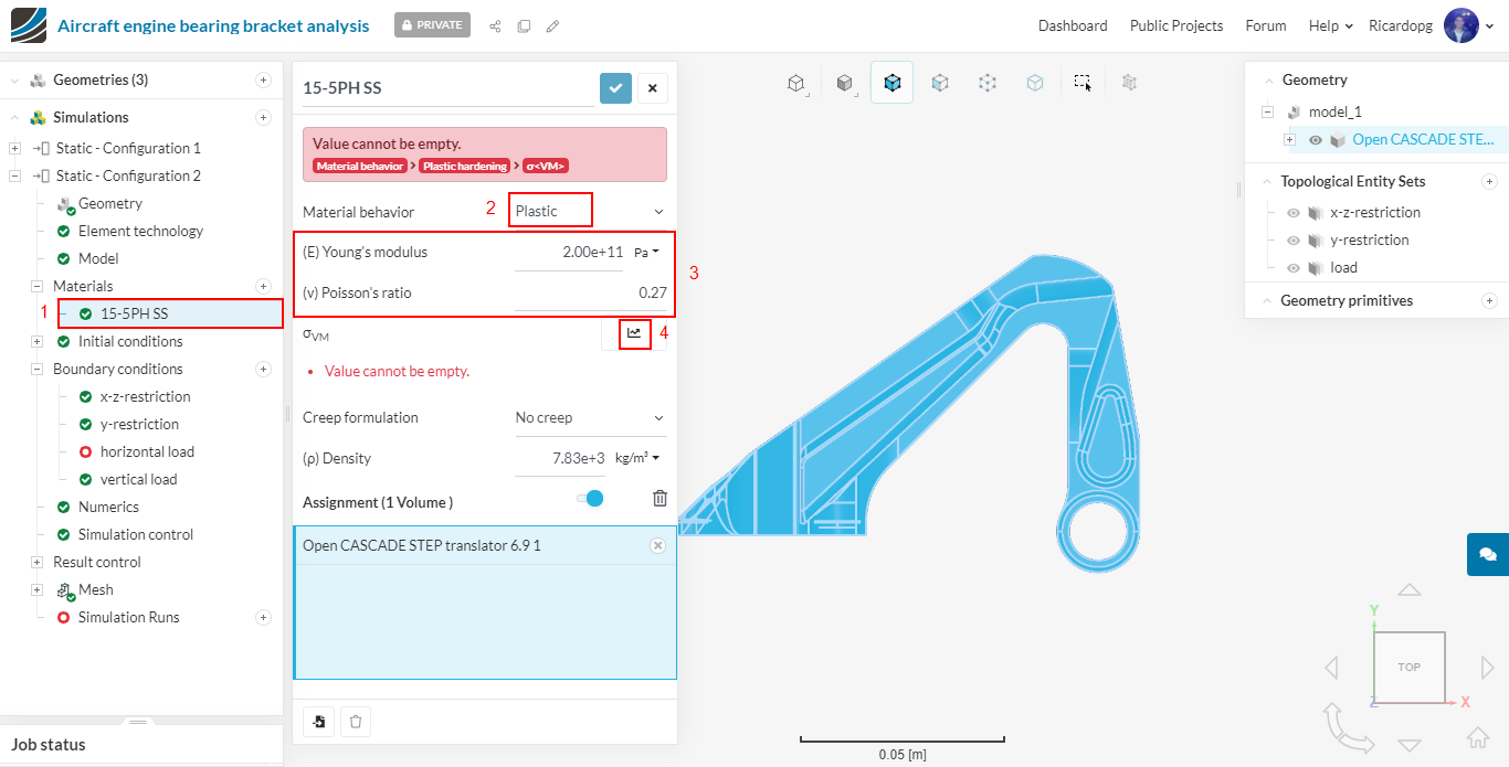
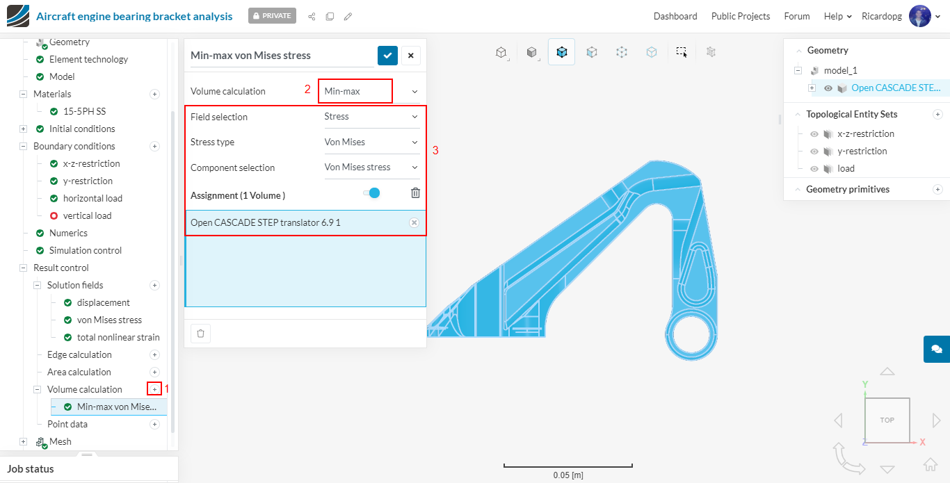
After clicking on the “arrow” next to σVM (step 4 from the image above), a panel will open up. Either drag your .cvs file or browse until you upload it. The table will automatically be loaded. Just hit Apply to continue.
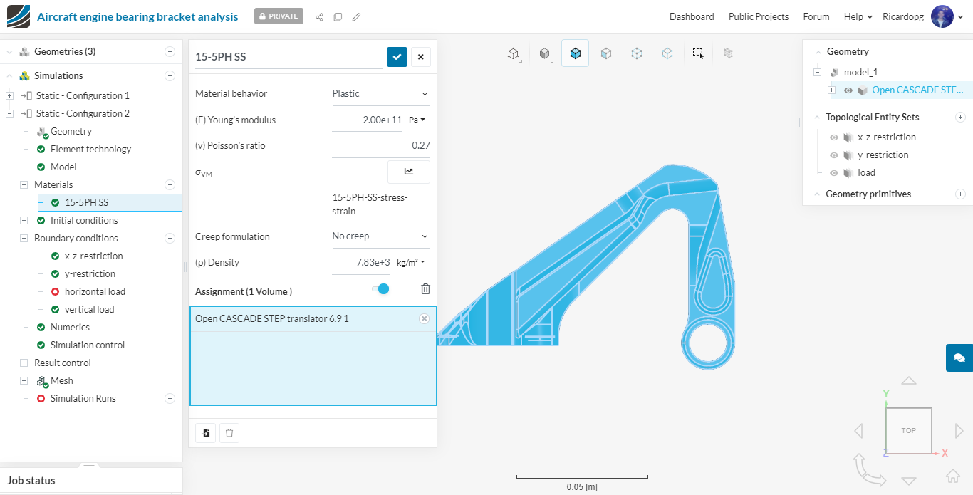
In the end, the 15-5PH SS should be looking like this:
Boundary conditions
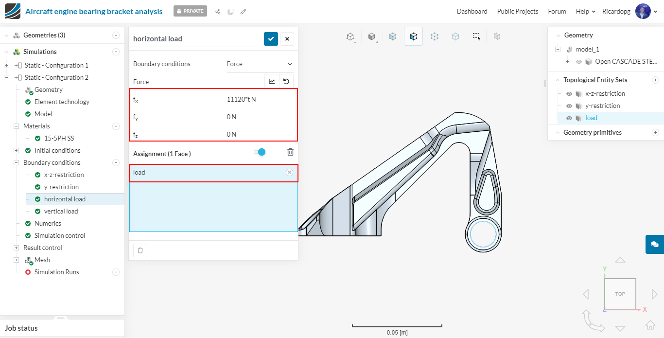
Next go to horizontal load and click on the small arrow to open up more options.
In the window that pops up, click on Formula. Give the value of 11120t* in the x direction. This will ramp the load over time (as solver doesn’t perform this automatically) and material nonlinearity will solved easily.
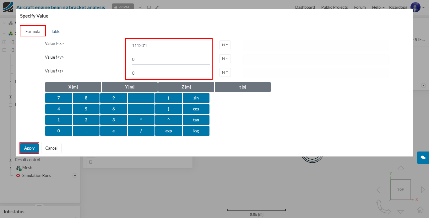
Assign this boundary condition to the load topological entity set:
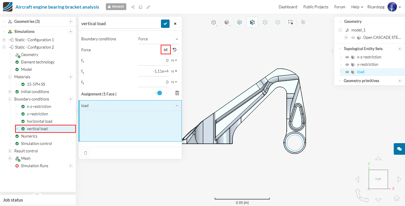
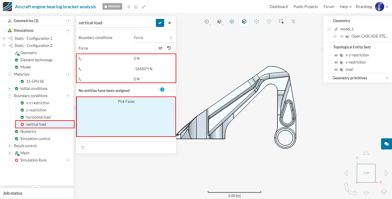
Next go to vertical load. A formula will also be input, but this time give it a value of -16680t* in the y direction.
Remember to unassign all faces for the first simulation:
Now please go to Simulation control and change Maximum time step length and Maximum runtime to 14400 seconds.
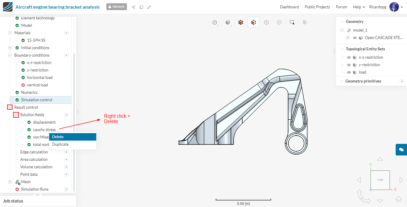
Go to Result control and delete cauchy stress (it can be found under Solution fields). It will save us some computation time:
We will create a new Volume calculation result control. It will be a Min-max type for von Mises stress. Assign it to the entire volume:
That’s it for the non-linear case. Proceed to Simulation Runs and Start. Name it e.g. Configuration 2 - Horizontal load.
Vertical load case: follow the same steps from the first simulation (assigning load to the vertical load and leaving horizontal load without assignments). Name the vertical load simulation run Configuration 2 - Vertical load.
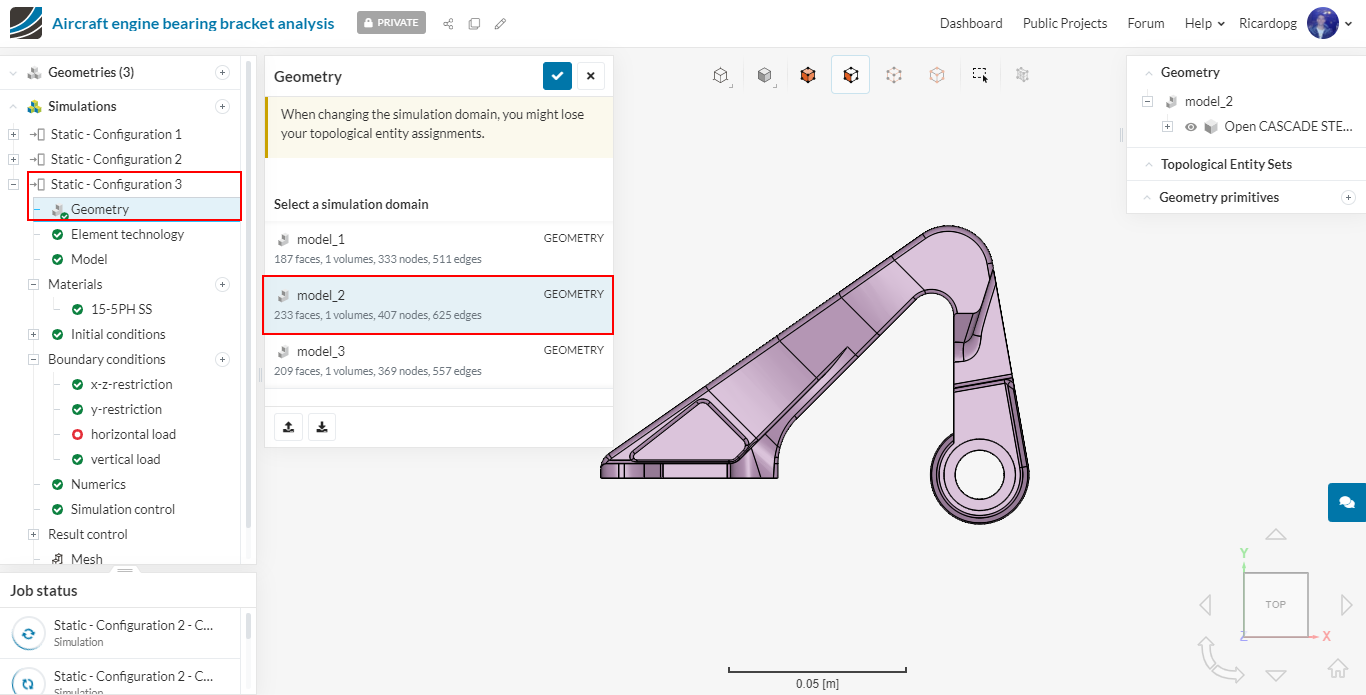
Configuration 3: For configuration 3, duplicate the first simulation i.e. Static - Configuration 1 and rename it Static - Configuration 3 (optional). Change the Geometry to model_2. It should look like this:
Follow all the above steps in order to create topological sets and assign them back to boundary conditions. Make sure that you first assign load set to horizontal load while un-assigning load from vertical load.
Afterwards, create a new run and rename it to Configuration 3 - Horizontal load and click Start.
For the vertical load case, please follow the above steps. Create a new run and rename it to Configuration 3 - Vertical load and click Start.
Configuration 4: For configuration 4, duplicate the second simulation i.e. Static - Configuration 2 and rename it Static - Configuration 4 (optional). Change the Geometry to model_2.
Please also make sure to assign volume to von Mises stress in bearing bracket’ under Volume calculations in Result control (all assignments are lost upon changing geometry).
Create a new run and rename it to Configuration 4 - Horizontal load and click Start.
For the vertical load case, please follow the above steps. Create a new run and rename it to Configuration 4 - Vertical load and click Start.
Configurations 5 & 6: please do all the same as above, but this time assigning the model_3 to Geometry.
Post-processing
Post-processing of linear cases (Configurations 1, 3 and 5). Here we will show results for the horizontal load cases.
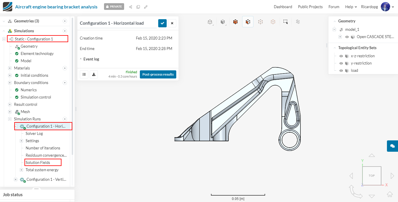
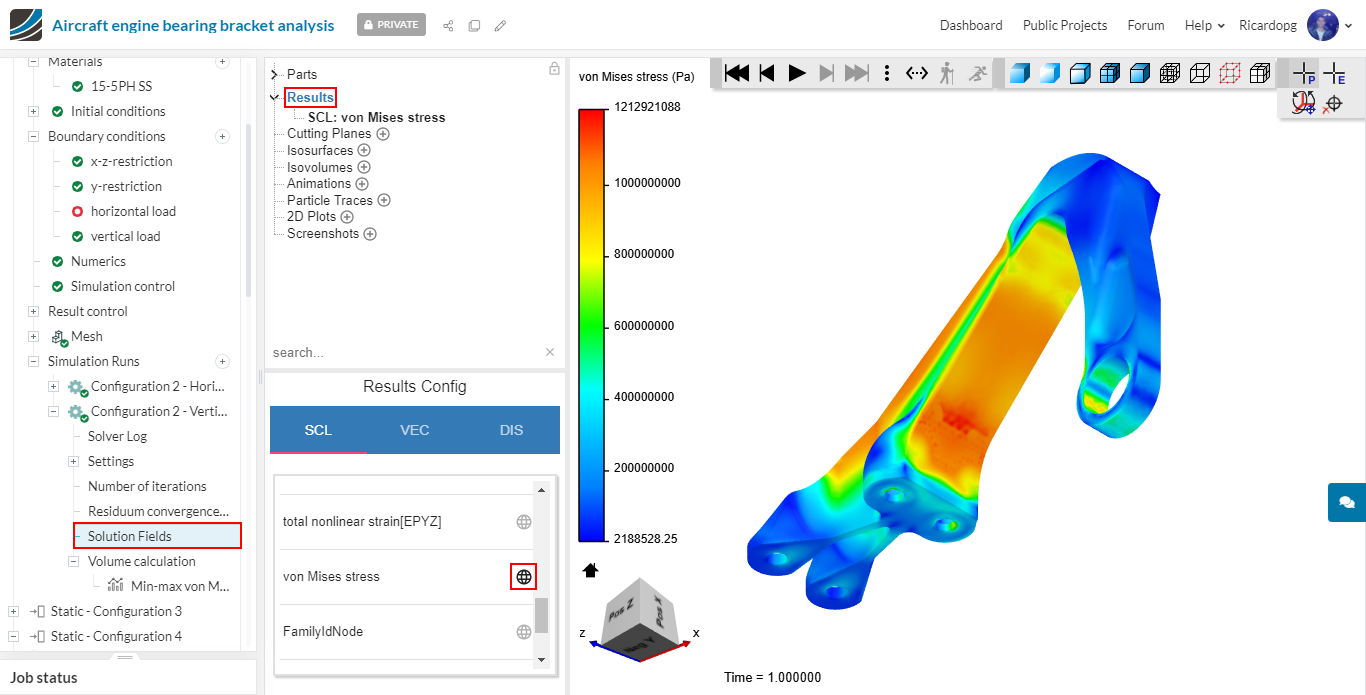
When the simulations finish running, head over to the post-processing environment by selecting a simulation and clicking on Solution Fields:
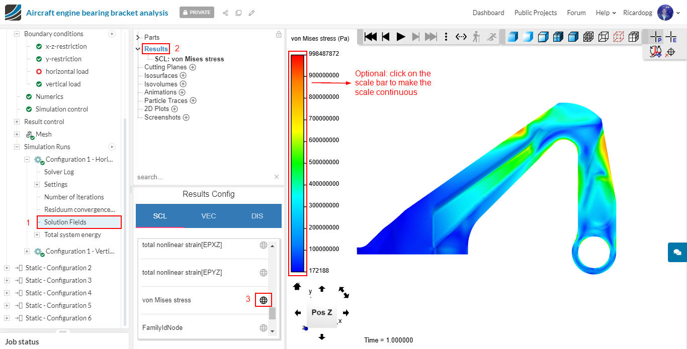
Select the scalar von Mises stress to be plotted by clicking on Results.
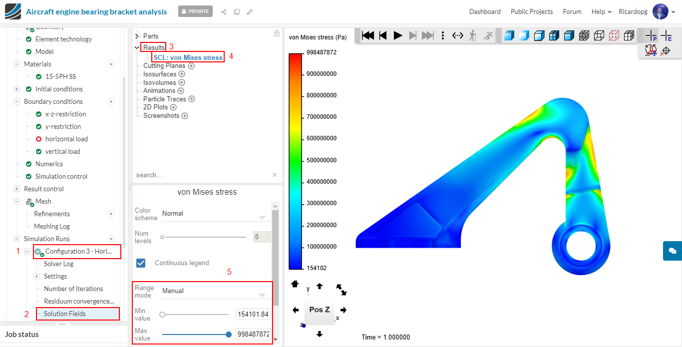
Repeat this process for configurations 3 and 5 (with horizontal load). To make the comparison easier, manually change the scale range so that the maximum stress is the same as the one seen in the first configuration.
Configuration 3 - Horizontal load:
Configuration 5 - Horizontal load:
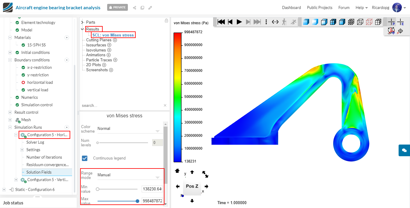
Visually inspect the 3 cases in different angles to see the differences between them in terms of von Mises stress.
For the horizontal load that was applied, models 1 and 3 experienced similar maximum von Mises stress (indicated by the maximum value from the scale bar in automatic range). It was just short of 15-5PH SS’ yield stress (1e9 Pa). Model 2 experienced stresses of nearly 9e8 Pa.
Perform similar post-processing for Configurations 1, 3 and 5 with vertical load.
Now we will look in to the post-processing of the nonlinear cases. We will do the post-processing of configuration 2 with vertical load. Same steps can be followed to perform the post-processing for the other non linear cases.
- Min/max von Mises stress volume calculation:
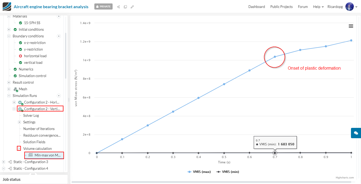
After the entire prescribed load has been applied, model_1 is being subjected to over 1.2 GPa, about 20% above its yield stress. Regions close to the support bolts are under the most stress.
Now change the scalar field from von Mises stress to All displacement.
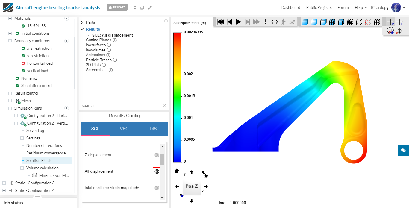
By switching to the DIS tab and enabling displacement, the model will deform to the state that it would be as a result of the load applied to it.
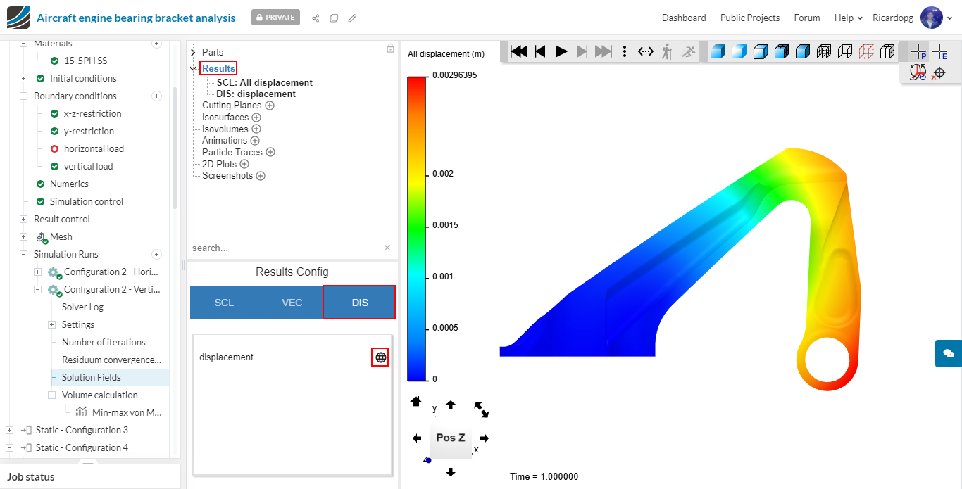
Perform similar post-processing to the other nonlinear configurations and compare the results!