Recently I was asked if it was possible to simulate ice build on the leading edge of a NACA0012 wing using SimScale and the help of LEWICE with its GUI front LEWINT. I am therefore writing this post to share my learning experience and workflow I used.
As a bit of a disclaimer, LEWICE is not free, there is a two week trial afterwhich you will need to purchase a licence. LEWINT which is the user interface for LEWICE is available here.
Geometry for LEWICE
What I thought was a straightforward step was actually not that straight forward. LEWICE requires a file upload of the aerofoil (or shape) in coordinates as a .xyd file, which I had never heard of before. But despite the odd file type, the coordinate system is the same as the .dat file type downloaded off of many online aerofoil libraries. To get the correct format download the .dat file edit it in a text editor by removing the top line (with text) and saving it as the .xyd file type.
Setting up the analysis
- On the home screen click ‘set the analysis path’ and select the directory for the analysis and results.
- Next set the geometry, add a name. It’s best to stay away from symbols etc. Click the geometry box and find your define .xyd file. Next to this, specify the cord length. Define the thermal ice protection as no protection.
- Setting up the flight configuration requires some data which you will need to define, if you are unsure what these values are this is an excellent Resource,
- In atmospheric conditions you will also need some more values that can be found in the above resource or will have defined some yourself. I used the ‘Lang-a’ distribution.
- Ensure that you name both the flight configuration and the atmospheric setup.
- Go to ‘Run’, the only thing I changed was number of steps. This isn’t very computationaly expensive so I changed it to 200. Select run, tick the box in the top left corner and then return. Say yes to solving 1 run.
- Once the run has finished head over to plot results, tick the x/c box and view final shape. If you recieve a warning saying the file cannot be uploaded it will probably be an issue with your geometry upload.
This is the data I used for this simulation:
Altitude = 2400m
Freestream velocity = 66.7 m/s
Temperature = -5°C
Droplet size = 25 micrometer
Cloud liquid water content (LWC) of 0.5 g/m
Accreation time = 2700s
AoA = 5 degrees
Cord = 2m
The tutorial for LEWINT is a bit clunky, but it does take you through an example setup.
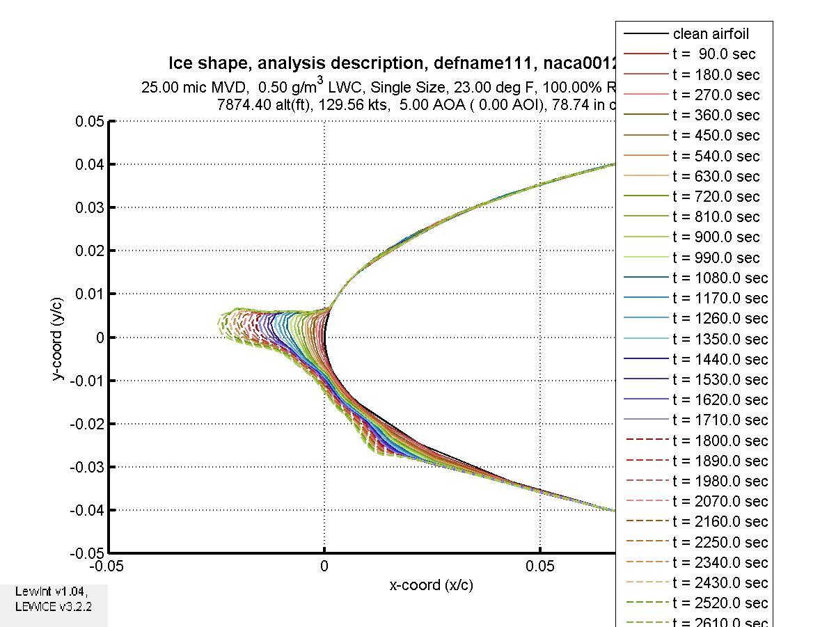
Below is the ice build up over time, this can be used to produce different profiles for different time steps or there is a final ice buildup plot available if your only interested in the ice build up at a set time.
Creating the 3D geometry in OnShape
This part is actually very easy if you are willing to use OnShape and my profile importer script. Firstly import my profile importer script here. Next you will need to request your geometry profile be uploaded to the script (just sent me a message with file location). Once I have uploaded it you will need to update the script link to the new version. That is all for the prerequisits, next is geometry creation. The file you will need it something like name.final.dat, or you will need to take a data set from the timestep file and save each data set as a different .csv for file upload.
To start the geometry all you will need is a straight line as long as the cord length that you used for your analysis, in my case it was a 2m cord. Next using my importer script select the ice profile from the drop down list, then select the leading and trailing points (either end of the line) and if the profile is inverted tick the flip option. It should look something like this:
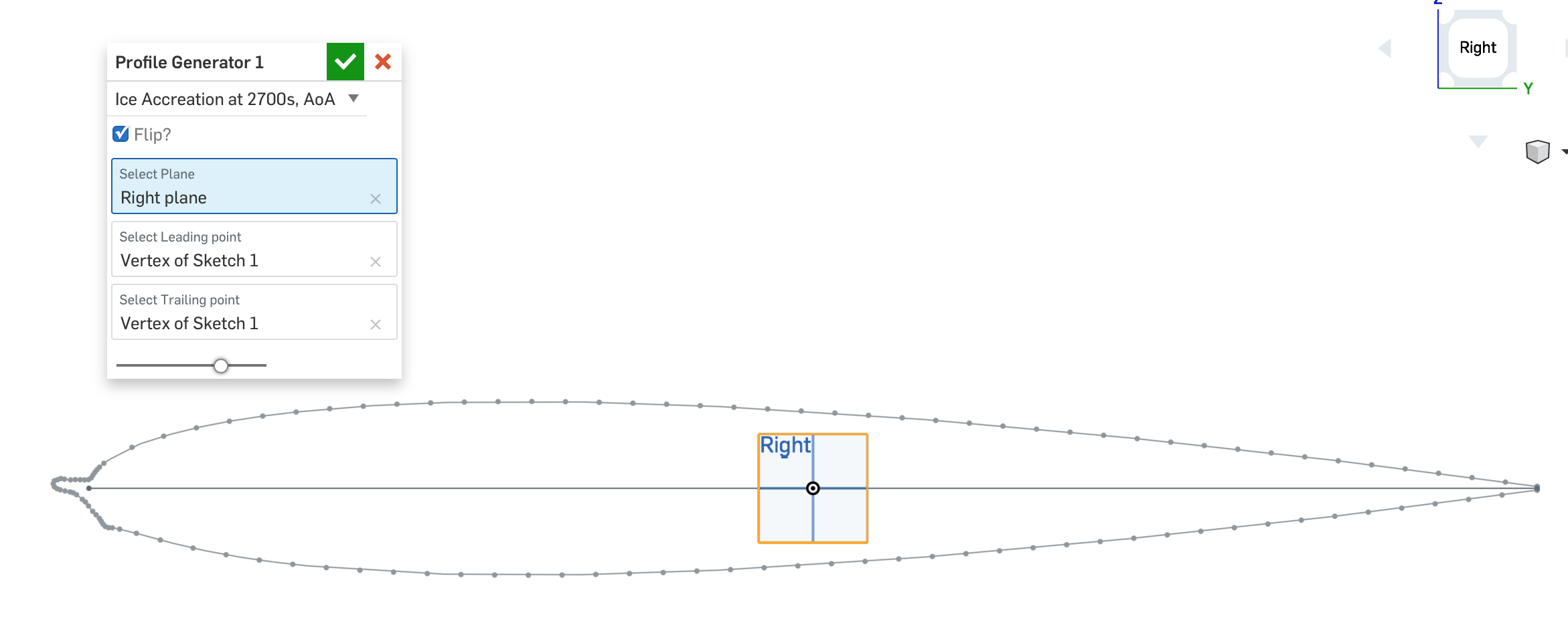
The problem with using .dat files from online libraries is that the trailing edge is often open, you will need to close it using a line. After this simply Extrude the geometry.
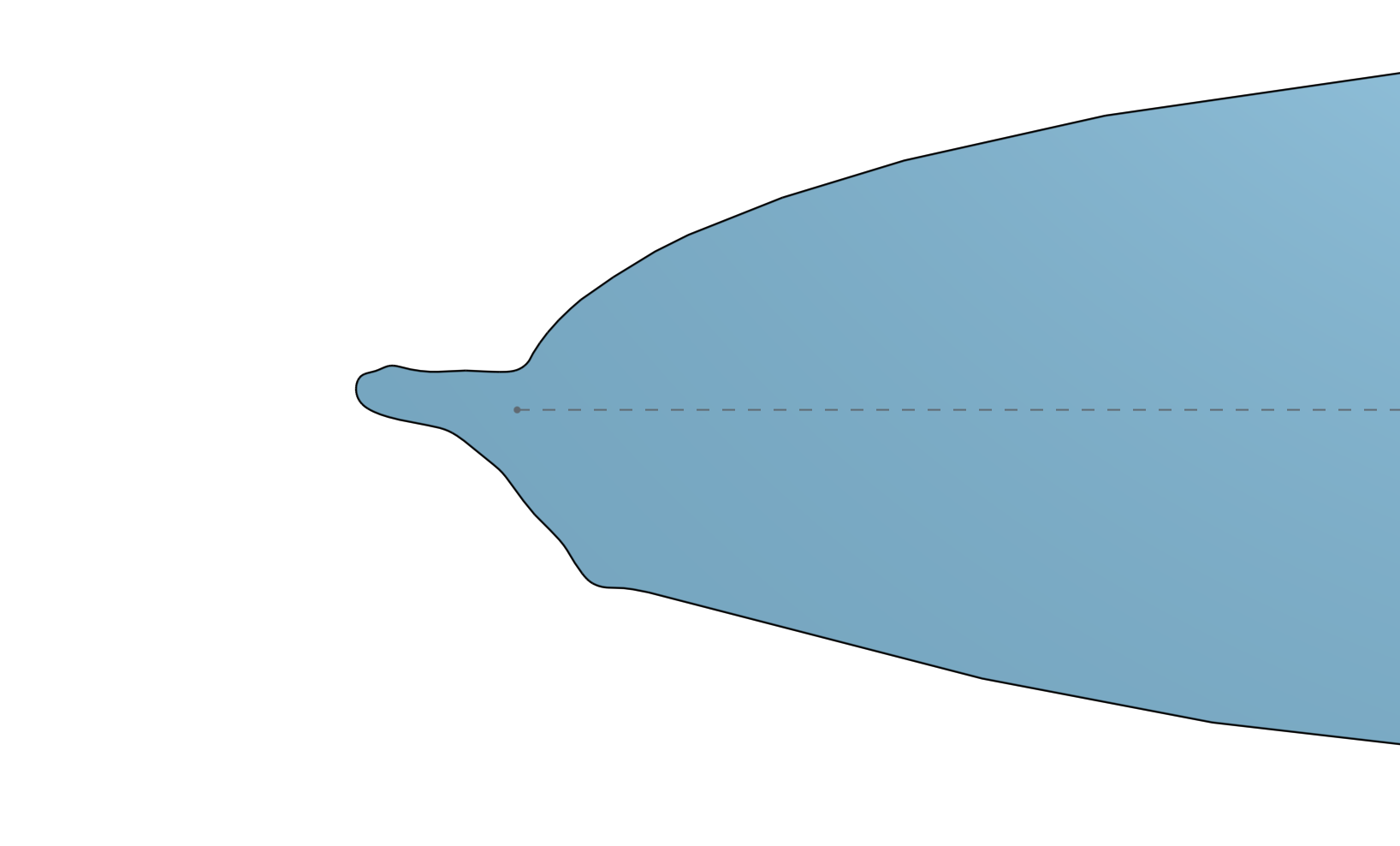
The Geometry is now ready for importing into SimScale so we can see how this ice affects the performance of the aerofoil.
Analysis in SimScale
Now it gets interesting, we are going to use SimScale to compare how the iced NACA 0012 performs against a clean one. I am going to use an incompressable flow setup with k-omega SST turbulance model. First step is create a project and import the geometry from OnShape.
Meshing
For the mesh I am going to use a mesh that is good for any angle of attack, althought the cell count is a little higher the mesh setup is pretty general. Feel free to look at my mesh.
As we are using a wall function boundary condition for the wing we need to ensure that y+ is somewhere in the region of 30 to 200. This is quite an iterative problem where we create a good approximation run to rough convergence then look at the y+ results re-mesh and run again doing this until we have a mesh that we are happy with. Although the first mesh was good I preferred mesh 3:
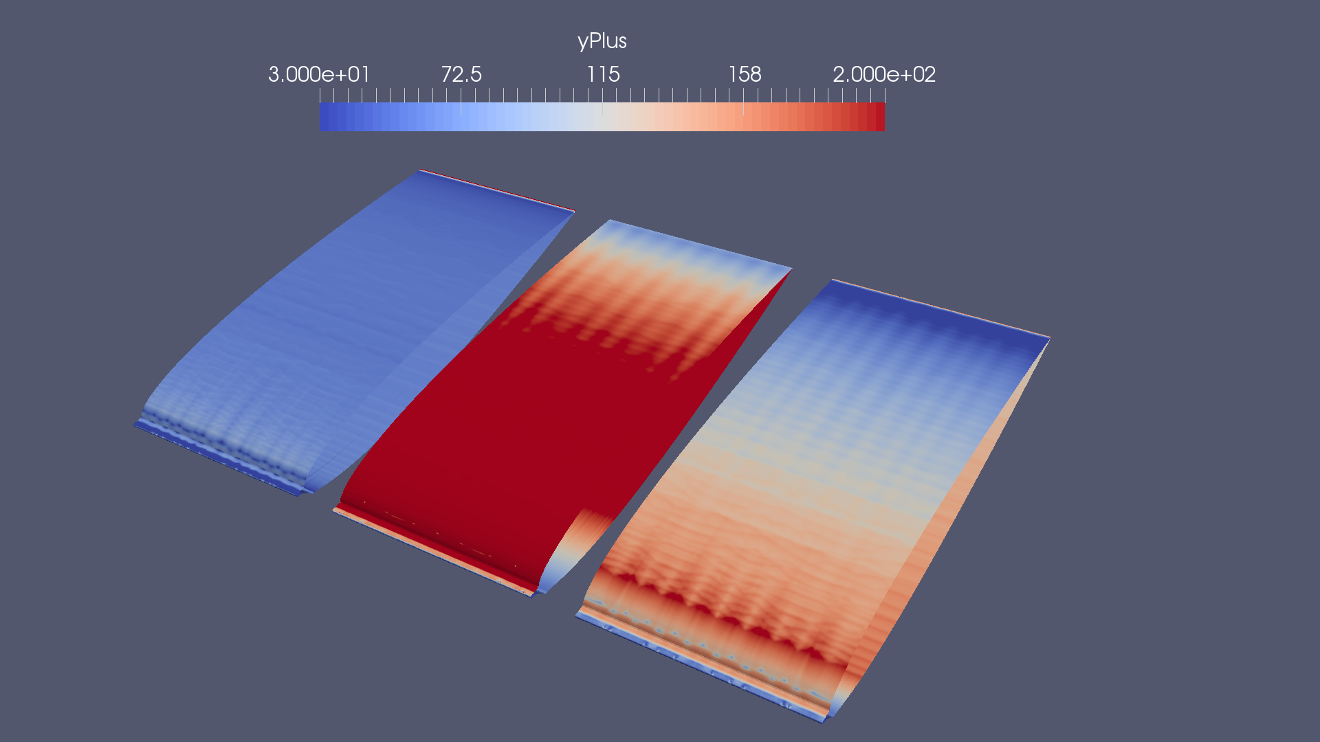
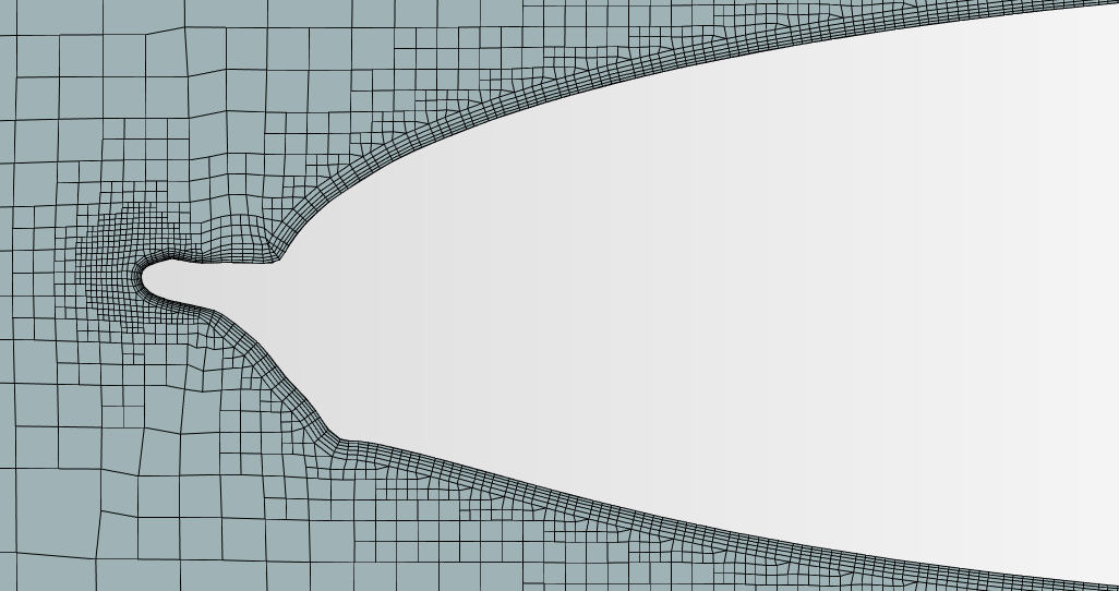
Here is a close up of the mesh used for the Iced aerofoil:
Simulation Setup
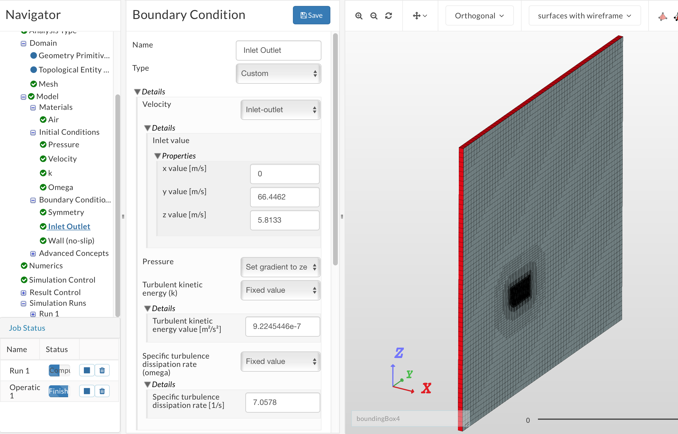
I like to setup aerofoil simulations with inlet-outlet boundary conditions around the outside of the mesh. This allows me to simply change a few parameters to alter the angle of attack (calculating the parameters using the MATLAB script below). Here is how I define my Inlet- outlet:
Matlab Code
velocity = 66.7;
angle = 5;
xVelocity = 0;
yVelocity = velocitycosd(angle);
zVelocity = velocitysind(angle);
x_Lift_Direction = 0;
y_Lift_Direction = cosd(angle+90);
z_Lift_Direction = sind(angle+90);
x_Drag_Direction = 0;
y_Drag_Direction = cosd(angle);
z_Drag_Direction = sind(angle);
Velocity = [xVelocity,yVelocity,zVelocity]
Lift_Direction = [x_Lift_Direction,y_Lift_Direction,z_Lift_Direction]
Drag_Direction = [x_Drag_Direction,y_Drag_Direction,z_Drag_Direction]
The sides of the domain should a be symmetry to simulate the wing being an of infinate length, and the walls of the aerofoil should be no slip wall functions. Again feel free to look at my setup.
To analyse the lift coeficient of the two conditions we need to specify a result control item ‘force coefficients’ using the lift direction and drag direction normal and paralel to the flow (this is also produced by the above MATLAB code).
Results
Firstly looking at the coefficients plot’s for each case (with and without icing) we can see that as expected the aerofoil with no ice build up is more efficient than the aerofoil with an ice build up:
Clean Aerofoil:
Lift Coeficient = 0.457
Drag coeficient = 0.036
Cl/Cd = 12.694
Aerofoil with ice:
Lift Coeficient = 0.425
Drag coeficient = 0.043
Cl/Cd = 9.884
 good luck,