
In fluid dynamics, incompressible flow refers to a flow in which the density remains constant in any fluid parcel, i.e. any infinitesimal volume of fluid moving in the flow. This type of flow is also referred to as isochoric flow, from the Greek isos-choros (ἴσος-χώρος) which means “same space/area”. It is important to underline the difference between an “incompressible flow” and an “incompressible fluid”: while the first is a characteristic of the flow, the second is a characteristic of the material. All fluids are apriori compressible but many are considered to be incompressible because the density variation is negligible for common applications. Incompressibility is a feature exhibited by any fluid under certain conditions. In Table 1, a set of different cases is shown, to highlight the independency between the usual definition of the fluid and the characteristics of the flow.
Table 1: Examples of flow compressibility for different fluids.
Continuity Equation
Flow in a Pipe
Let’s consider a fluid flow in a closed pipe. Consider now the volume of the flow contained between two sections of the pipe, as shown in figure 1. The continuity equation, in a Eulerian framework, is the analysis of the mass transfer across the boundary sections of this volume.
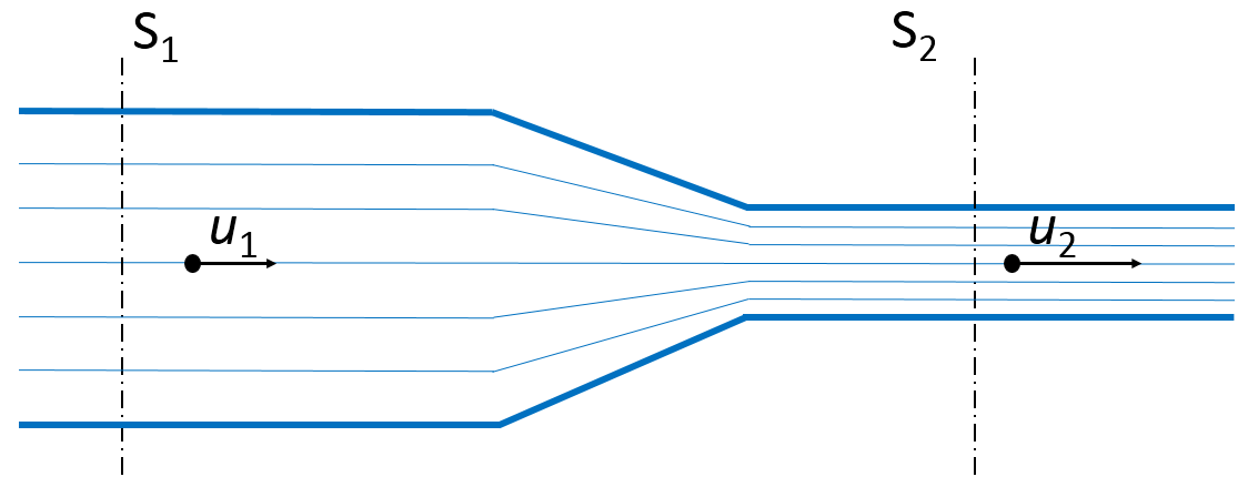
Figure 1: Fluid flow in a pipe
Since no mass creation or deletion can occur within the pipe, the variation of mass contained in the domain can be written as:
where m is the total mass in the domain, \Delta m_1 is the inward mass flux and \Delta m_2 is the outward mass flow. The total mass can be written as:
where \rho is the fluid density and V_e is the volume of the examined portion of the pipe. Under the hypothesis of incompressible flow (\rho constant) and non-deformable pipe (V_e constant), equation (2) implies that m is constant, so:
By developing equation (3), we obtain:
where A_i is the area of the i-th section, \Delta t is the time interval, and u_1 and u_2 are the inward and outward velocities respectively. Finally, the continuity equation can be rewritten as:
for any couple of sections, where F is the fluid flow rate.
This analysis is valid for real pipes (with solid walls), but also “virtual” pipes, i.e. groups of streamlines with no mass exchange across the lateral surface, which is always the case for laminar flows. “Virtual” pipes can also be seen as streams which do not diffuse or mix with the rest of the flow.
The principle of conservation of the fluid flow rate is why tap jets decrease their section while falling (figure 2): the falling liquid accelerates due to gravity, thus the section of the flow decreases proportionally.
In this section, we have focused on real or virtual pipes of finite dimension, but we can also shrink the pipe to an infinitesimal dimension until it basically coincides to a single streamline. This way, we could extend the principle of conservation of the fluid flow rate to any continuous problem, as shown in the following paragraph.
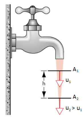
Figure 2: Flow rate conservation for tap flows ^3
Differential Formulation
The same procedure done for the flow in a pipe can be done for a fluid flow in any given domain. The first step consists of imposing the conservation of the mass, i.e. that the variation of the mass in the domain is equal to the net mass flow across the boundaries. This means that no mass creation or deletion occurs in the domain. Thus, the conservation equation can be written as:
where m is the mass of the domain, (u\rho) is the mass flux across the boundaries, and S is the boundary of the domain.
By using the Gauss’ theorem (or divergence theorem), the surface integral can be rewritten as a volumetric integral defined in the domain \Omega:
The mass of the fluid can be obtained by integrating the density, thus equation (8) can be rewritten as follows:
Hence, the conservation equation can be reduced to:
which is valid for both compressible and incompressible flows.
Let’s now impose the incompressibility hypothesis. Incompressibility requires any fluid particle to have a constant density, which is mathematically expressed by the material derivative of the density:
We can now rewrite equation (10) in terms of material derivatives:
By replacing the incompressibility condition (equation (11)) in the new form of the continuity equation (equation (13)) we obtain:
Equation (14) shows that, for incompressible flows, the incompressibility condition is respected for any divergence-free velocity field. Thus, the imposition of a constraint on the density (equation (11)) is equivalent to the imposition of a constraint on the divergence of the velocity field.
Dependency on the material parameters
The conditions for which an incompressible flow occurs vary depending on the material properties of the fluid. Any fluid can be considered as incompressible under certain conditions on velocity and pressure. The tendency of a fluid to change volume when subjected to an external load depends on the material itself. For the sake of simplicity, let’s consider the common case of an elastic isotropic material$^4$. The volumetric stiffness can be expressed as:
where p is the pressure, \rho is the density, and K is the bulk modulus. The bulk modulus measures the stiffness of a material to volumetric loads or, in other words, the pressure required to produce a reference volumetric strain. The higher K is, the higher the pressure variations must be to induce a compressible flow. Table II reports the bulk modulus for some materials; from this table we deduce that water will behave as a compressible fluid only if huge variations in the pressure occur (e.g. water hammer), while air requires low variations in the pressure to be modelled as an incompressible fluid.
Table 2: Examples of bulk modulus for different materials ^5
In more practical terms, water will require a pressure gradient 15000 times higher than air to exhibit the same density variation (animation 1), thus it is more likely to behave as an incompressible flow in common applications.
Animation 1: Different weight needed to induce a 10% variation in density in an 1 cm^2 piston with different materials.
The volumetric stiffness can also be expressed through the Poisson ratio (\nu), which is directly linked to the bulk modulus ^6:
where E is the Young modulus. For incompressible fluids (i.e. K\rightarrow+\infty) the Poisson ratio tends to \nu=0.5. It is common, for incompressible flows, to use \nu instead of K in order to be able to express this limit situation. On the other hand, \nu=0.5 may lead to several numerical issues (e.g. locking) which require special simulation techniques to be solved$^{7,8}.
While K and \nu measure the volumetric stiffness, a measure of the material’s compressibility is given by the inverse of the bulk modulus:
where \beta is the compressibility of the material.
This value can be expressed in relation to the speed of sound c, since:
where the subscript S means that the transformation must be isentropic. Hence, equation (17) can be rewritten as:
Dependency on the Mach number
As seen in the previous section, the compressibility of a flow depends on the speed of sound in the material. In aerodynamics (or, in general, for any case in which two materials flow at different velocities), the compressibility of the flow can be expressed as a function of the Mach number, defined as:
where u is the relative velocity.
The conservation of momentum equation can be written as:
By substitution of equations (18) and (20) in the conservation momentum equation, we obtain:
This means that for low values of the Mach number, high velocity variations are required to produce a variation in the density, thus the flow tends to be incompressible. Experimentally, the incompressible behavior of the flow occurs for M<0.3, which corresponds to a change in density lower than 10%^9.
Applications
Incompressible flow modelling is used for a large amount of applications in CFD. The most common example is the simulation of liquid flows — especially water, due to its high bulk modulus. Free surface (figure 3) and fluid-structure interaction (figure 4) problems are examples of incompressible flows thanks to the relative low gradient in the pressure of the liquid. But also under-pressure flows (figure 5) can be treated as incompressible, as far as the fluid has a sufficiently high volumetric stiffness.
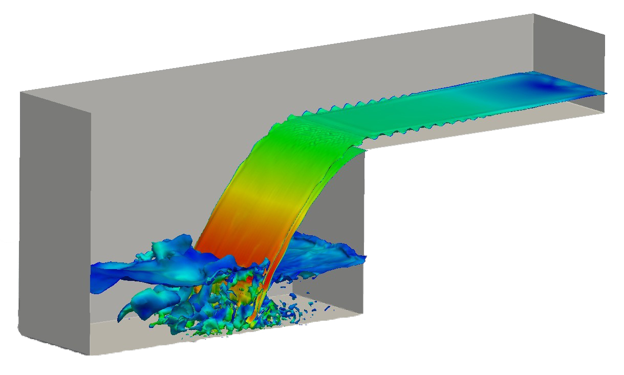
Figure 3: Free surface flow
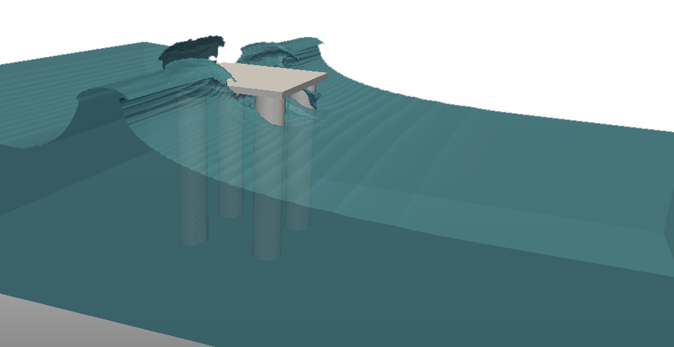
Figure 4: Fluid structure interaction
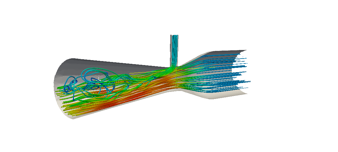
Figure 5: Incompressible flow in a Venturi injector
But incompressible flows are commonly used also in aerodynamics/hydrodynamics of vehicles, in which many applications have a low Mach number M<0.3(figure 6). Also for extreme cases like aerodynamics in F1 , the velocity is not high enough to make the compressibility relevant (the record velocity in F1 is 372.5 km/h ^{10} corresponding to M=0.29 at T=40°C).
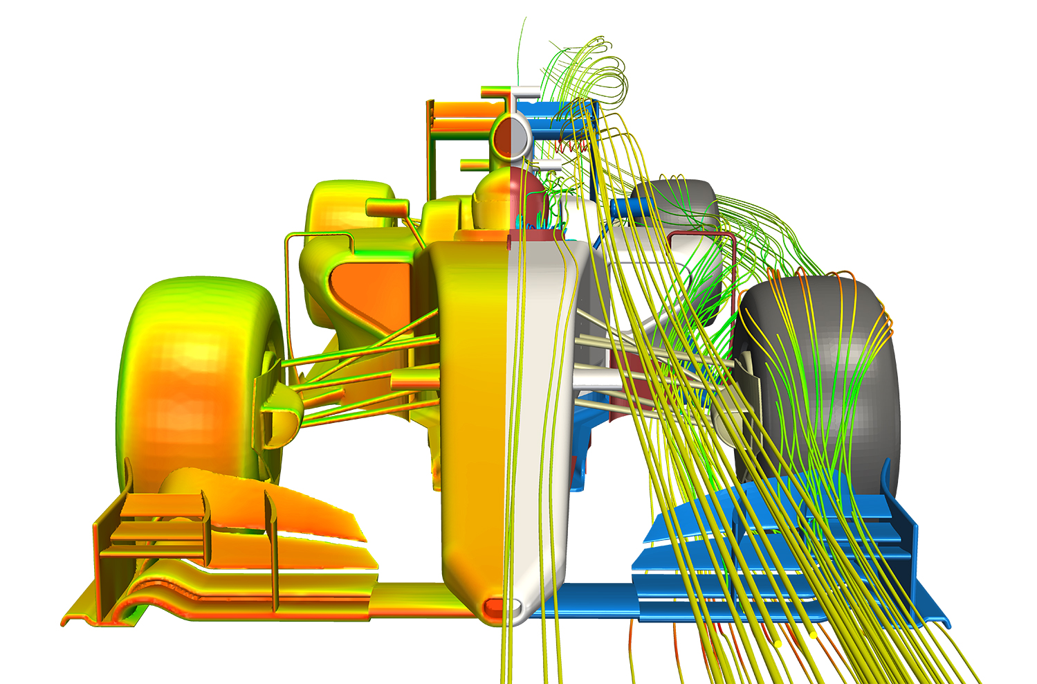
Figure 6: Example of aerodynamics at low Mach number: Air flow around a F1 vehicle$^{15}$
Related topics
- Compressible flow
- Linear elasticity
- Navier-Stokes equations
- Compressibility
- Mass transfer
- Boussinesq approximation
Resources
^2: mysite.du.edu/~jcalvert/tech/fluids/waterham.htm
^3: matfis.unisalento.it/c/document_library/get_file?folderId=6566673&name=DLFE-50238.pdf"
^4: http://www.brown.edu/Departments/Engineering/Courses/En221/Notes/Elasticity/Elasticity.htm
^5: http://www.engineeringtoolbox.com/bulk-modulus-elasticity-d_585.html
^7: http://mate.tue.nl/mate/pdfs/5513.pdf
^8: Hung, N.-X., Bordas, S. P. A. and Hung, N.-D. (2009), Addressing volumetric locking and instabilities by selective integration in smoothed finite elements. Commun. Numer. Meth. Engng., 25: 19–34. doi:10.1002/cnm.1098