'Tutorial : Turbulent Forced Convection' simulation project

[nelta]

I created a tutorial demonstrates the simulation of forced convection in a pipe: Turbulent Forced Convection

The physical problem to solve is that of a circular-cross section pipe with a heated section where a constant heat flux is added and with ambient air flowing into the pipe from the left with a uniform velocity.

The pipe geometry is

Length: 6.045m

Radius: 0.0294m

The mathematical model used to solve this problem is a boundary value problem.

The domain (or the geometry of the region of interest) is governed by a set of equations, namely conservation of mass, conservation of momentum, and conservation of energy, as well as the ideal gas law, k-conservation, and -conservation that need to be solved. Since there is heating in the pipe, the density is variable. Note from the governing equations that the flow is also turbulent. These two additions further complicate the governing equations. The model used to solve the governing equations is the k-epsilon turbulence model.

The boundary conditions are defined at the edges of the domain. For this problem, the boundary conditions are outlined below:

[nelta]

The following is a step-by-step tutorial for a turbulent convective heat transfer through a circular-cross section pipe simulation.

The workflow for the problem includes:

1. Preparing the CAD model for the simulation.

2. Setting up the simulation: Assigning Materials and Boundary Conditions

3. Creating the mesh

4. Running the simulation

5. Analyzing the results; Post-Processing.

1. Preparing the CAD model for the simulation

The CAD model was prepared from the pipe junction geometry found in the Tutorial 2: Pipe junction flow

SimScale Login

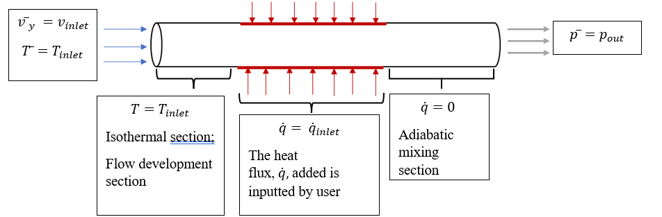
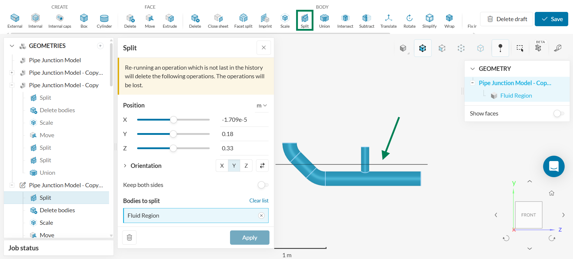
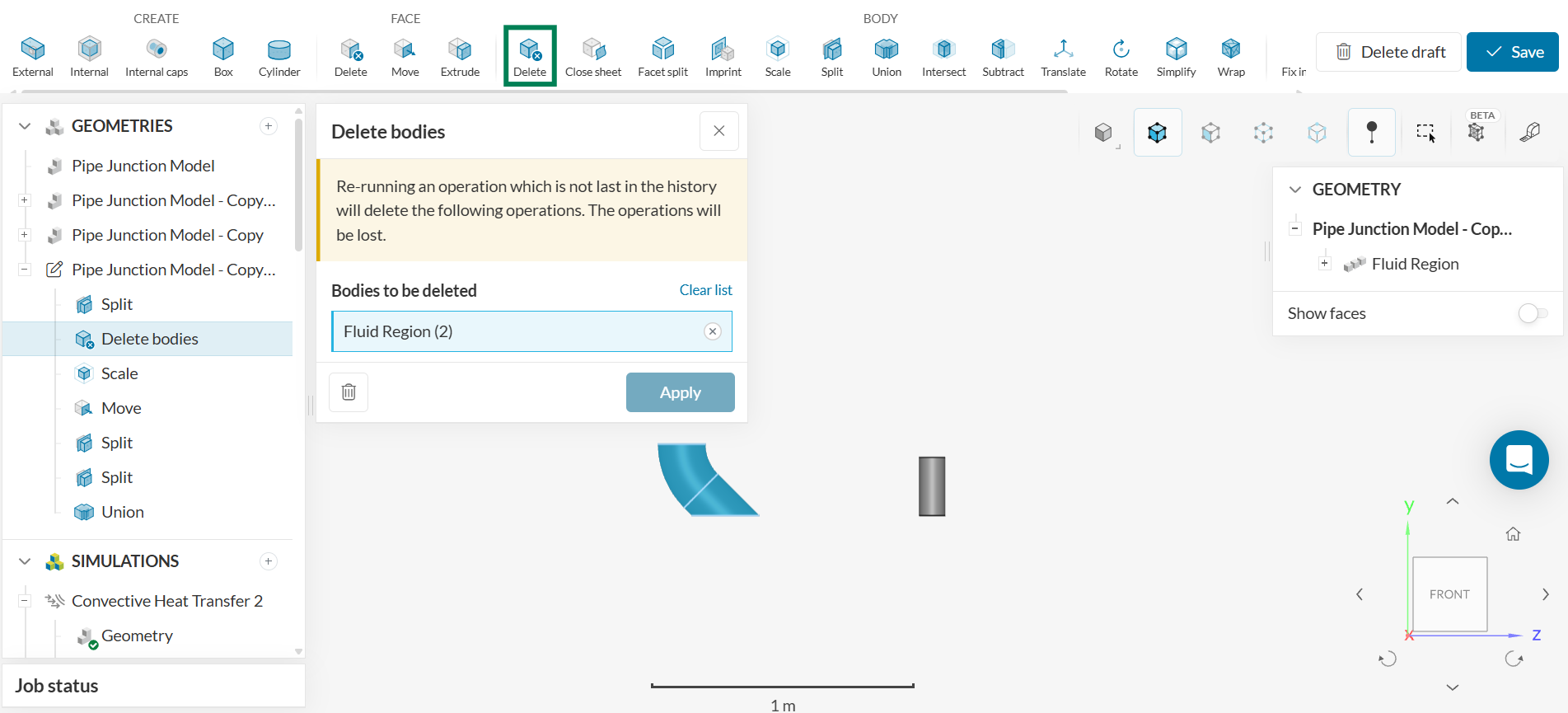
This pipe geometry already has a fluid region assigned to it. The fluid region is the domain of the problem and is the region where the fluid flows. Creating a fluid region is a crucial prerequisite to completing a SimScale simulation. Since a fluid region (specifically an internal flow volume) was already created for the pipe junction flow tutorial, this step does not have to be repeated and the CAD model can be edited to obtain the physical pipe geometry for this simulation. To modify the CAD model, click on ‘Edit a copy.’ Then, follow the remaining steps:

1. Click on the ‘BODY – Split’ operation to separate the vertical pipe highlighted. Select the ‘Fluid Region’ as ‘Bodies to split.’ Click ‘Apply.’
   
2. Perform the ‘BODY - Delete’ operation and delete the two bodies that are not the vertical pipe.

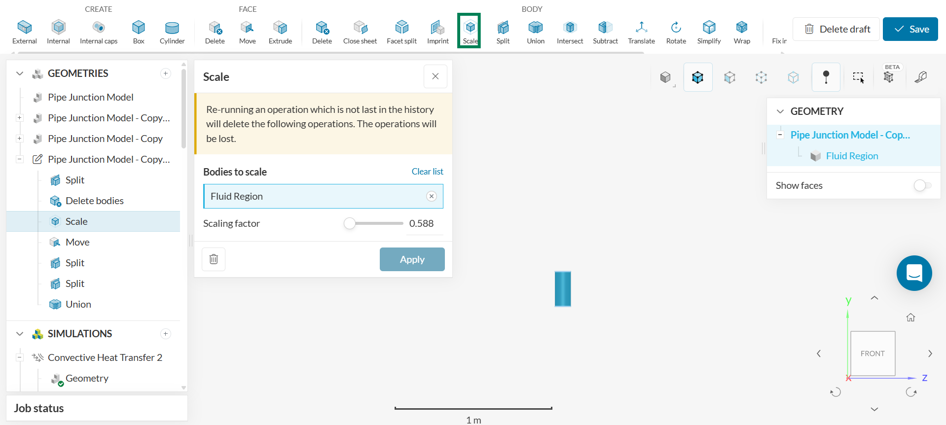
3. Perform the ‘BODY - Scale’ operation and set the scaling factor to 0.588.

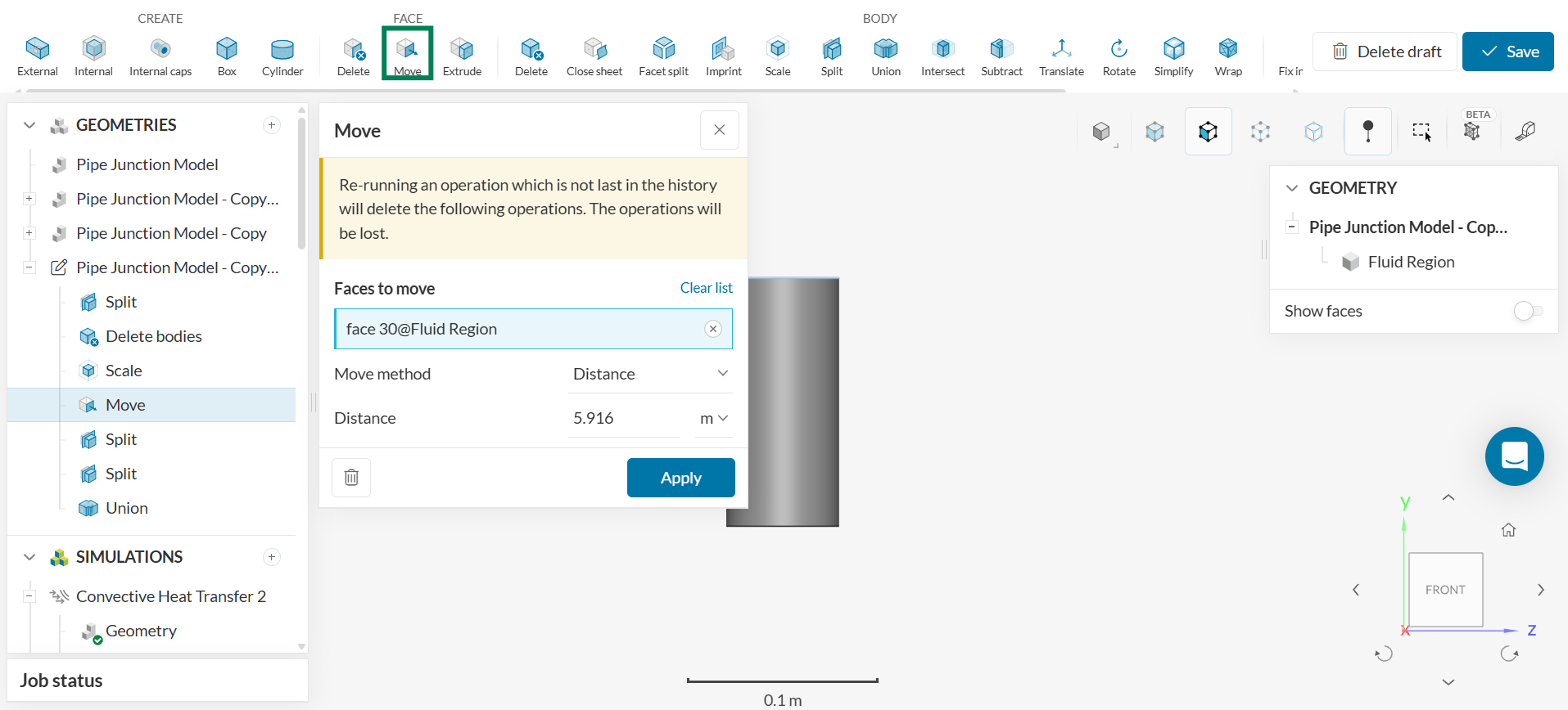
4. Select the ‘FACE - Move’ operation and click on the top face. Select ‘Move method- Distance’ and set ‘Distance’ to 5.916 m.

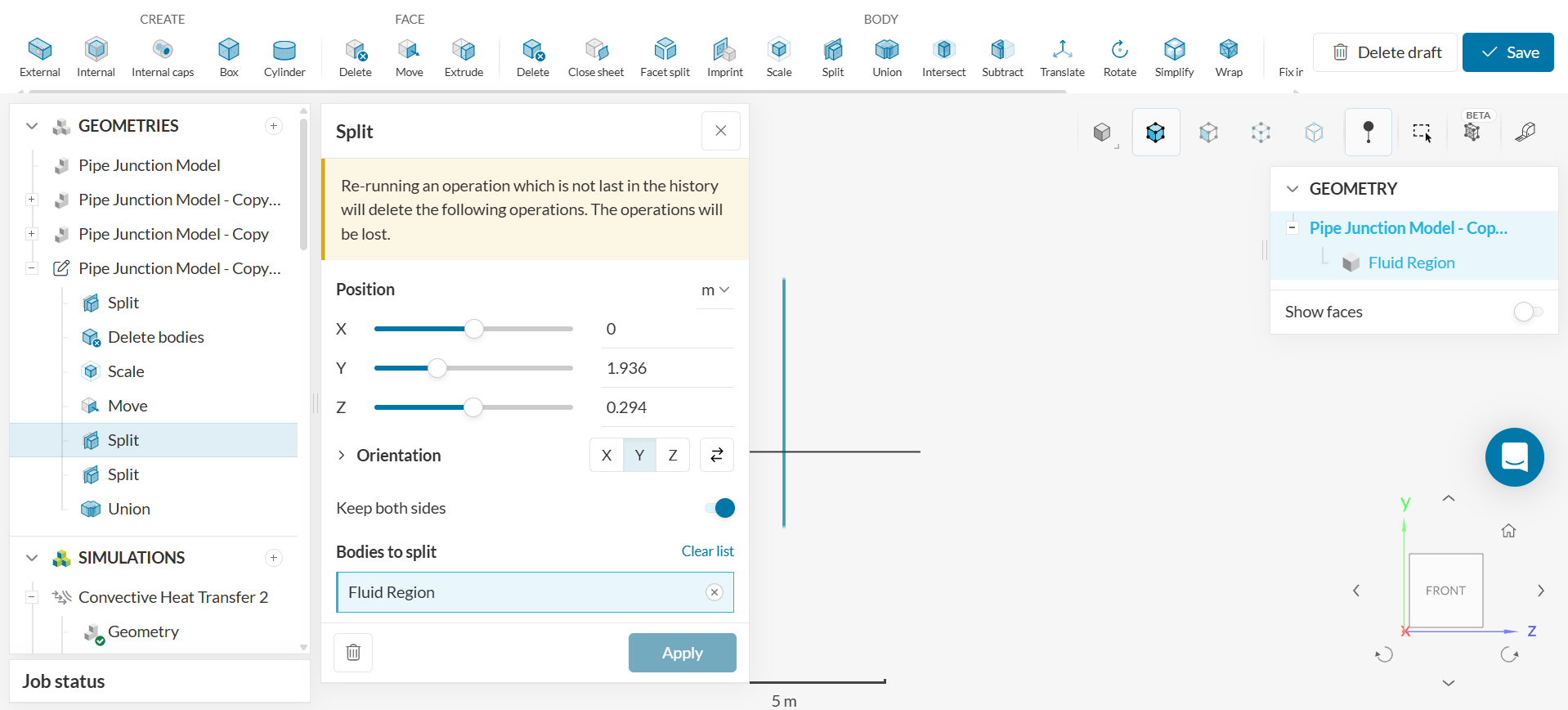
6. Perform the ‘BODY - Split’ operation and input the values given in the figure below.

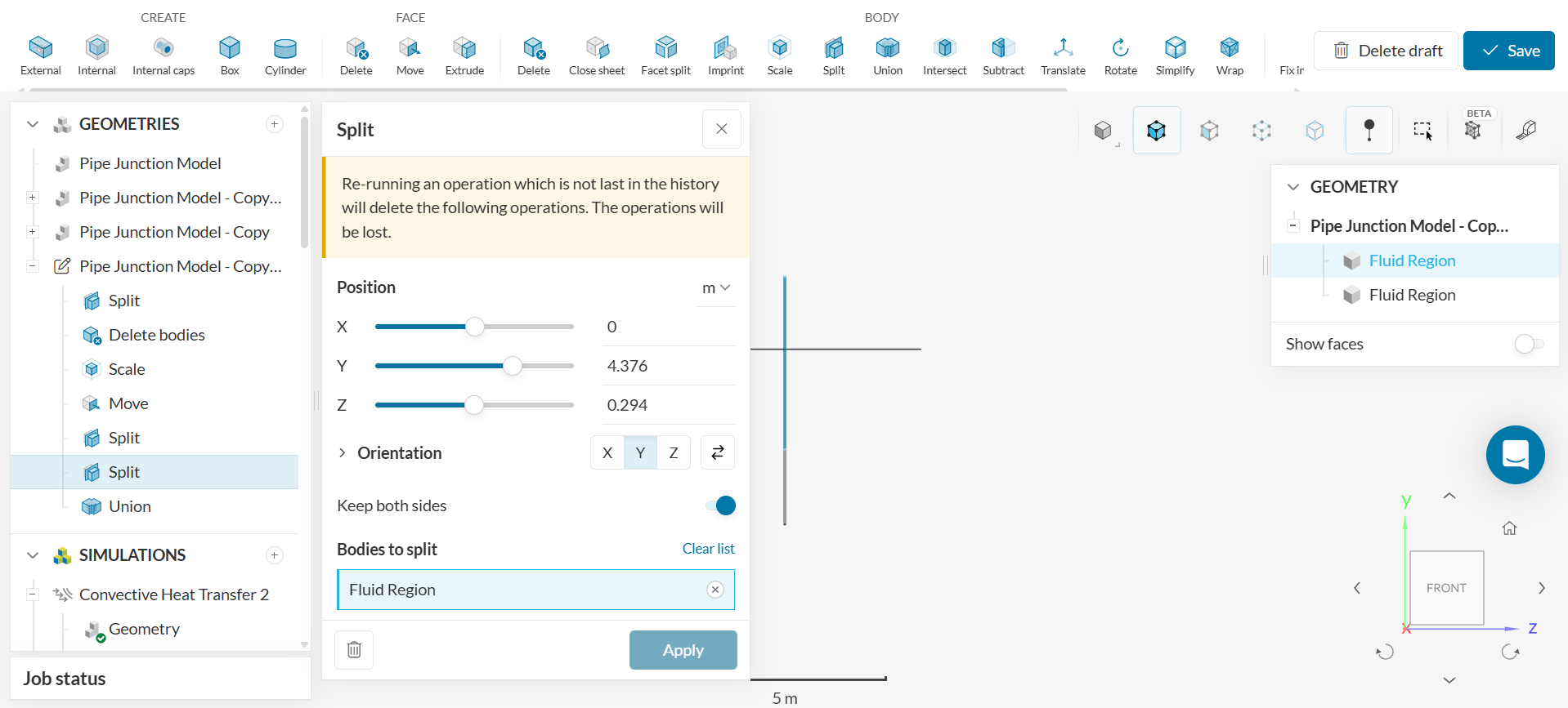
7. Perform the ‘BODY - Split’ operation a second time and input the value shown in the figure below.

8. Click on the ‘BODY - Union’ operation and select all three bodies to unite. Click ‘Apply.’

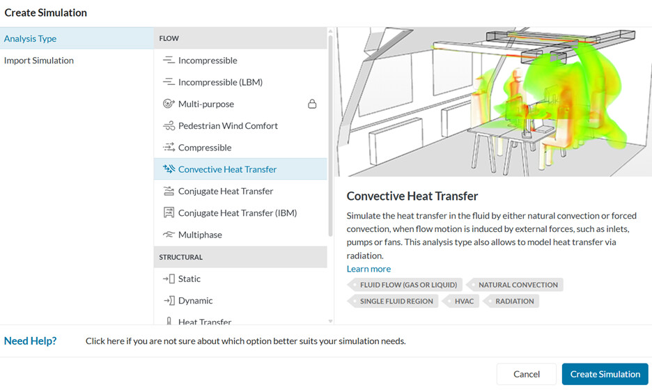
Save the draft. Select the ‘Convective Heat Transfer Analysis Type’ and click ‘Create Simulation.’

2. Setting up the simulation; Assigning Materials and Boundary Conditions

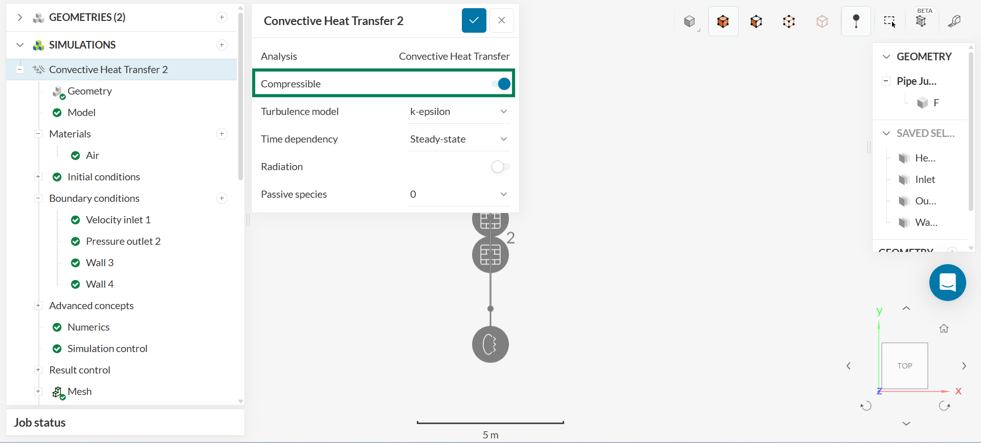
First, turn on the ‘Compressible’ toggle in the Convective Heat Transfer:

Set ‘Turbulence’ to ‘k-epsilon’.

To simplify the steps in setting up the simulation, create the following ‘Saved Selections.’ The ‘Select Face’ tool must be selected to create the saved selections.

1. a. Click on one of the circular cross sections of the pipe. b. Click on the ‘+ button’ to the right of ‘Saved Selections’ and name the selection Inlet. c. Click ‘Create new selection.’

2. Click on the other circular cross section of the pipe. Click on the ‘+ button’ to the right of ‘Saved Selections’ and name the selection Outlet. Click ‘Create new selection.’

3. Click on middle section of the pipe. Click on the ‘+ button’ to the right of ‘Saved Selections’ and name the selection Heated Section. Click ‘Create new selection.’

4. Click on the first section of the pipe adjacent to the Inlet face and click on the first section of the pipe adjacent to the Outlet face. Click on the ‘+ button; to the right of ‘Saved Selections’ and name the selection Wall 1 and 2. Click ‘Create new selection.’

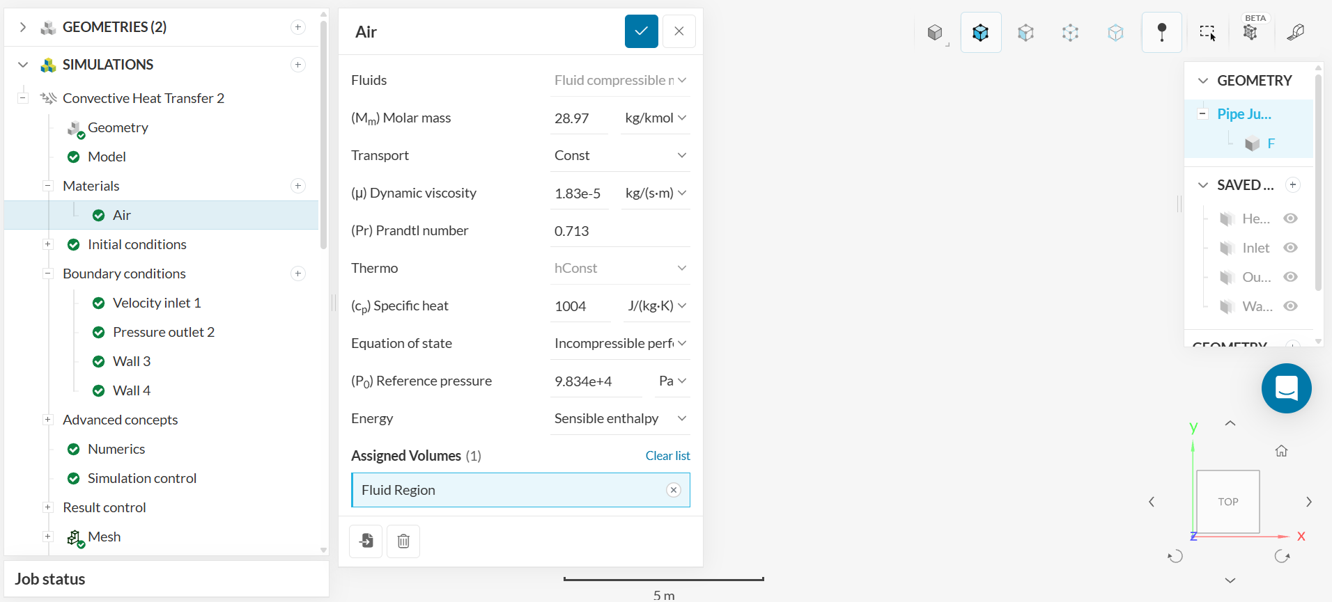
To assign a material to flow in the fluid region, click on the ‘+ button’ to the right of ‘Materials.’ Select ‘Air’ to be the material. Follow the settings in the figure below:

Be sure to set ‘Equation of state’ to ‘Incompressible perfect gas’.

The next step is to set up the ‘Initial Conditions’ of the simulation.

1. Leave the ‘Modified Gauge Pressure’ to the default value of zero.

2. Set the ‘Initial Conditions’ for ‘(U) Velocity’ to be into the Inlet face.

3. Considering the coordinate system presented in this tutorial, set 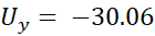. This represents the ambient air flowing from the left into the Inlet face.

4. Set the ‘Initial Conditions’ for the ‘(T) Temperature’ to be 298.15 K.

5. Set the ‘Initial Conditions’ for the ‘(k) Turbulent kinetic energy’ to be 3.388513 m^2/s^2.

6. Set the ‘Initial Conditions’ for the ‘() turbulent dissipation’ to be 6645m^2/s^3.

The next step is to assign the boundary conditions.

After hitting the ‘+ button’ next to boundary conditions, a drop-down menu showing different boundary conditions will appear.

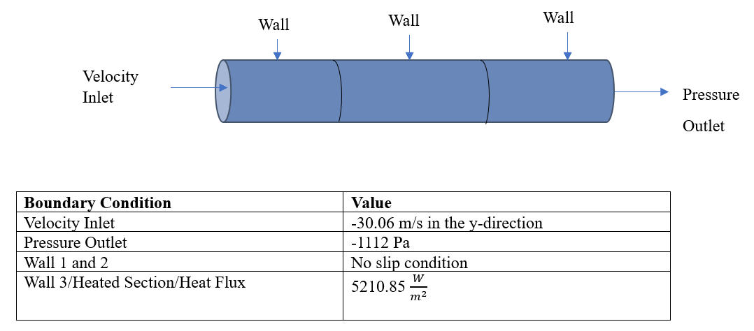
1. Assign a ‘Velocity inlet condition’ with . Assign the ‘Turbulence’ to be ‘Automatic.’ This considers a value of 0.05 for ‘turbulent intensity (I)’. The ‘turbulent mixing length (L)’ is calculated as 0.07D_h, where D_h is the hydraulic diameter of the boundary face. Set the ‘Temperature’ to 298.15 K. Assign the ‘Face’ to be the Inlet.

2. Assign a ‘Pressure outlet condition’ with a gauge pressure of -1112 Pa. Assign the ‘Face’ to the Outlet face.

3. Assign a ‘Wall boundary condition’ to Wall 1 and Wall 2. Set ‘(U) Velocity’ to ‘No-slip’, set the ‘Temperature type’ to ‘Fixed Value’, and set the ‘Temperature’ to 298.15 K.

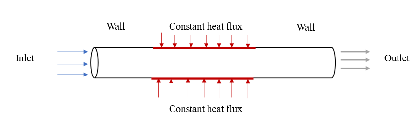
4. Assign a ‘Wall boundary condition’ to Heated Section. Set ‘Temperature Type’ to ‘Turbulent heat flux’ and ‘Heat source’ to ‘Flux heat source.’ Set ‘(q) Heat Flux’ to 5210.85 W/m^2. Keep the ‘Initial boundary temperature’ to 298.15 K.

The boundary conditions are summarized in the figure and table below:

Navigate to the ‘Simulation Control’ and set the ‘End time’ to 5500 seconds and ‘Delta t’ to 1. The number of iterations the simulation undergoes is given by End time/ Delta t.

Click on the ‘+ button’ next to ‘Result Control’ and click on the ‘+ button’ to the right of ‘Field calculation’ and select ‘Turbulence’ and ‘Wall shear stress’ so that these can be evaluated in post-processing.

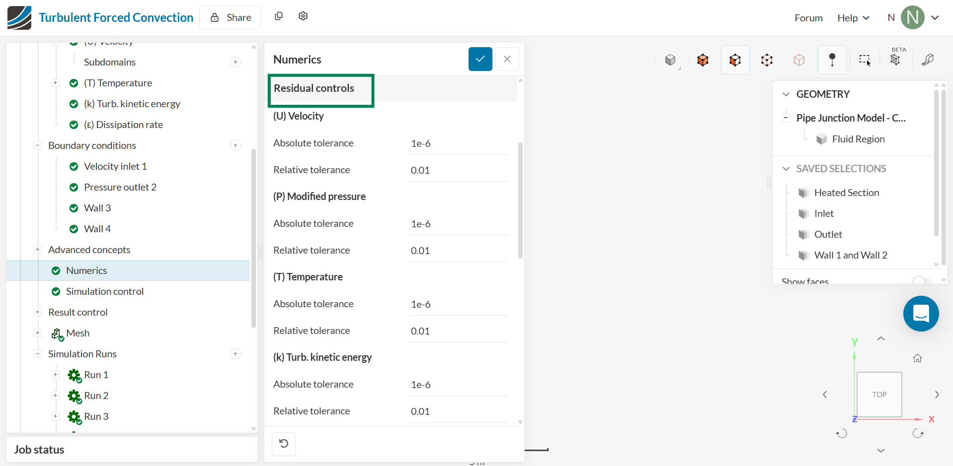
Navigate to ‘Numerics’ and set ‘Absolute tolerance’ to 1e-6 for ‘(U) Velocity’, ‘(P) Modified Pressure’, ‘(T) Temperature’, ‘(k) Turbulent kinetic energy’, and ‘() turbulent dissipation.’

3. Creating the Mesh

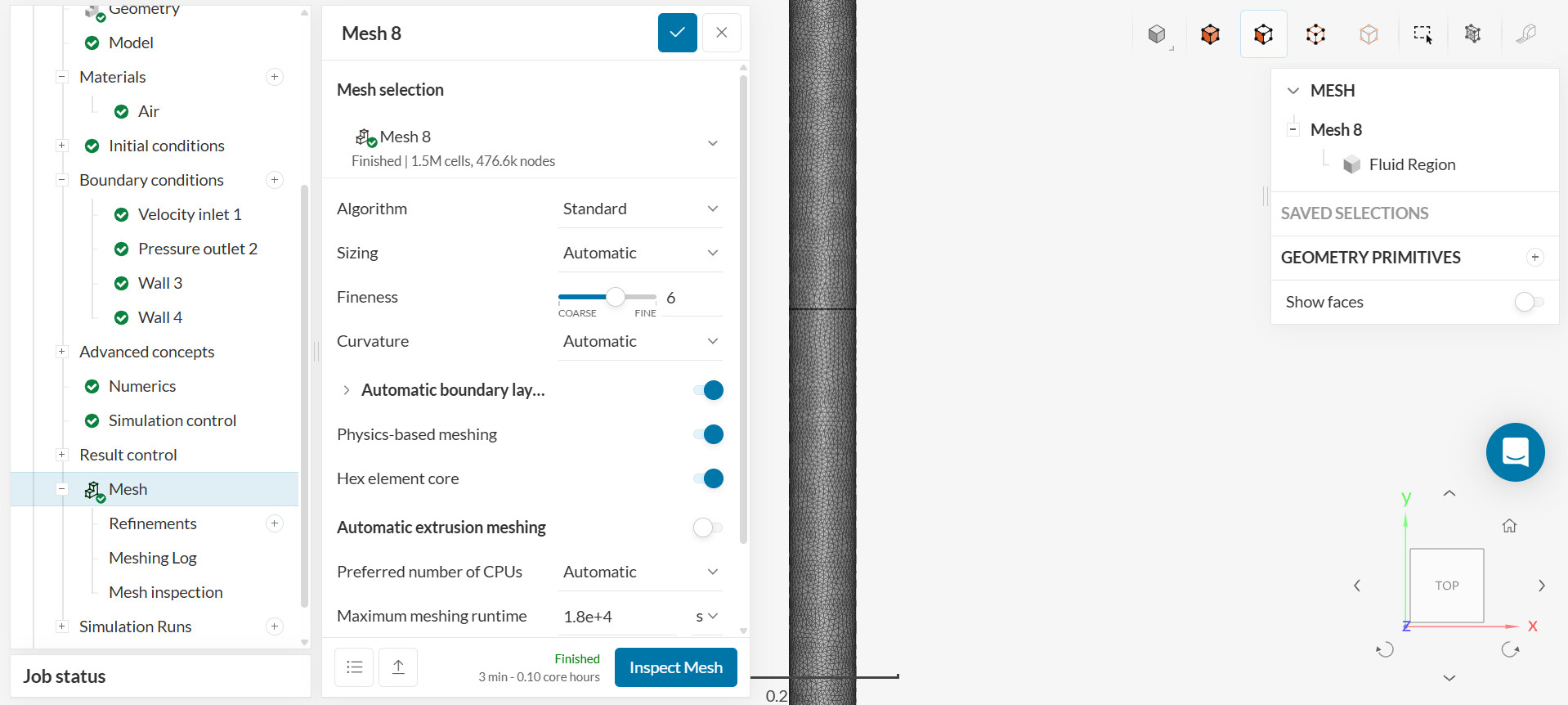
To generate the mesh, use the ‘Standard Algorithm.’ The Standard algorithm is generally a good choice for most geometries.

Change the ‘Fineness’ to 6. Click ‘Generate.’ The statistic for the generated mesh is 1.5 million cells and 476.6 thousand nodes.

Click on ‘Meshing Log’ to quickly inspect the mesh.

4. Running the Simulation

Click on ‘Run Simulation.’ The simulation should end in about 35 minutes and should spend around 9 core hours. The Run to refer to is Run 10.

5. Analyzing the Results; Post-Processing

Click on ‘Post-Processing.’

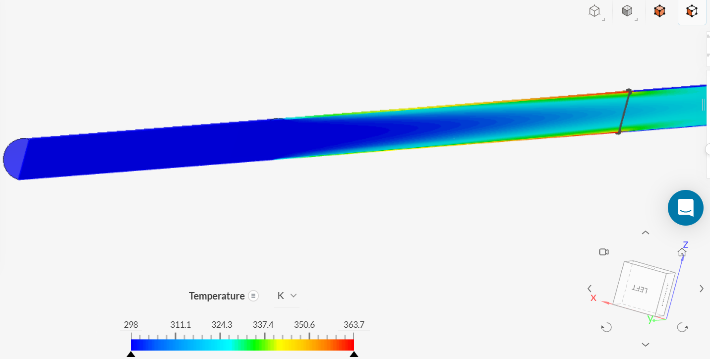
5.1. Temperature Contours

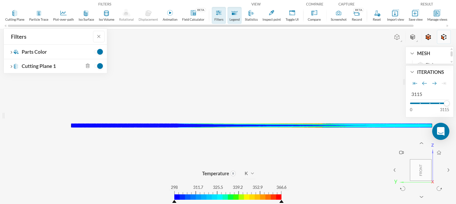
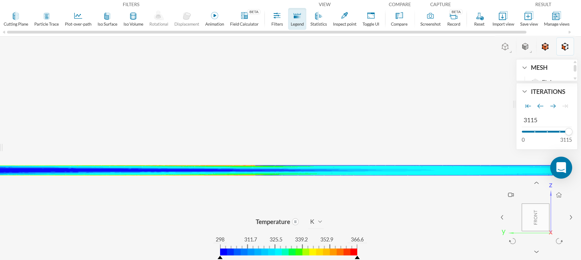
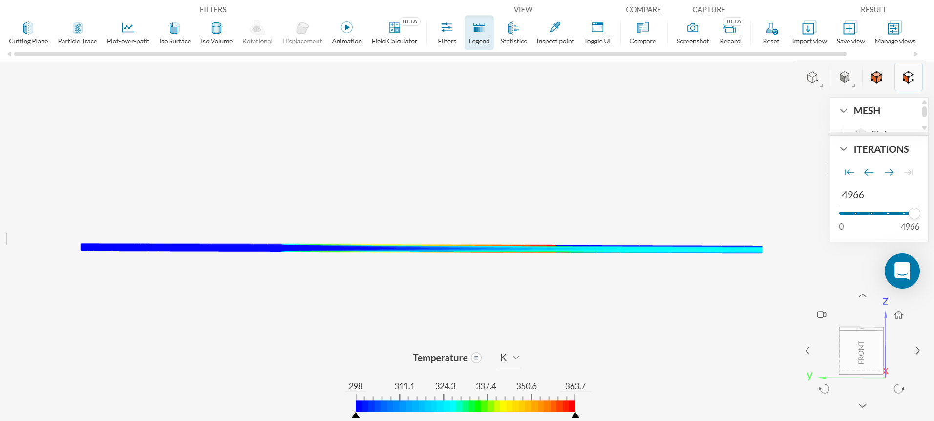
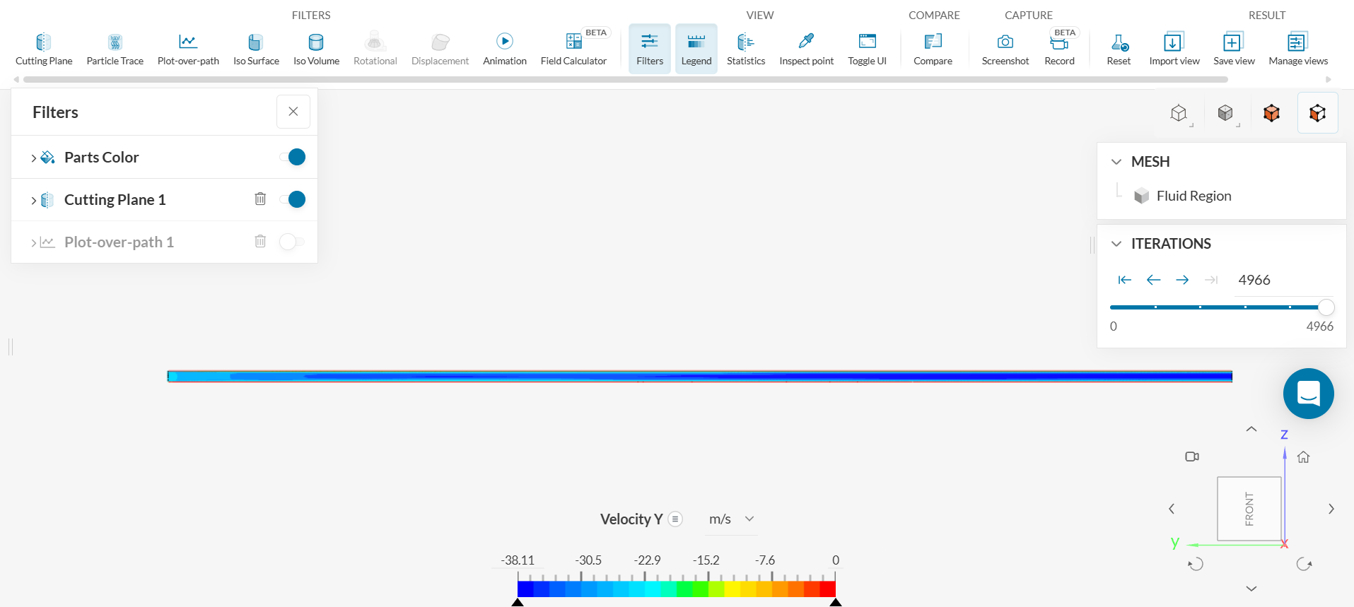
Click on “FILTERS - Cutting Plane” and change the ‘Orientation’ to X. Right click on the legend at the bottom of the screen and select ‘Division Number’ to be 35.

The first section shows an isothermal distribution with the uniform dark blue color. This region is the coolest region. The thermal boundary layer starts to form along the heated section of the pipe. It grows as the fluid moves downstream (toward the right). This section shows higher temperatures with red and orange near the surface and green and cyan color toward the middle of the pipe. This region is the hottest region. At the right end of the pipe where the heating ends, this third region is the adiabatic mixing region: the temperature shows to be nearly uniform in that region. Part of the heated and the third region of the pipe are shown in the figure below.

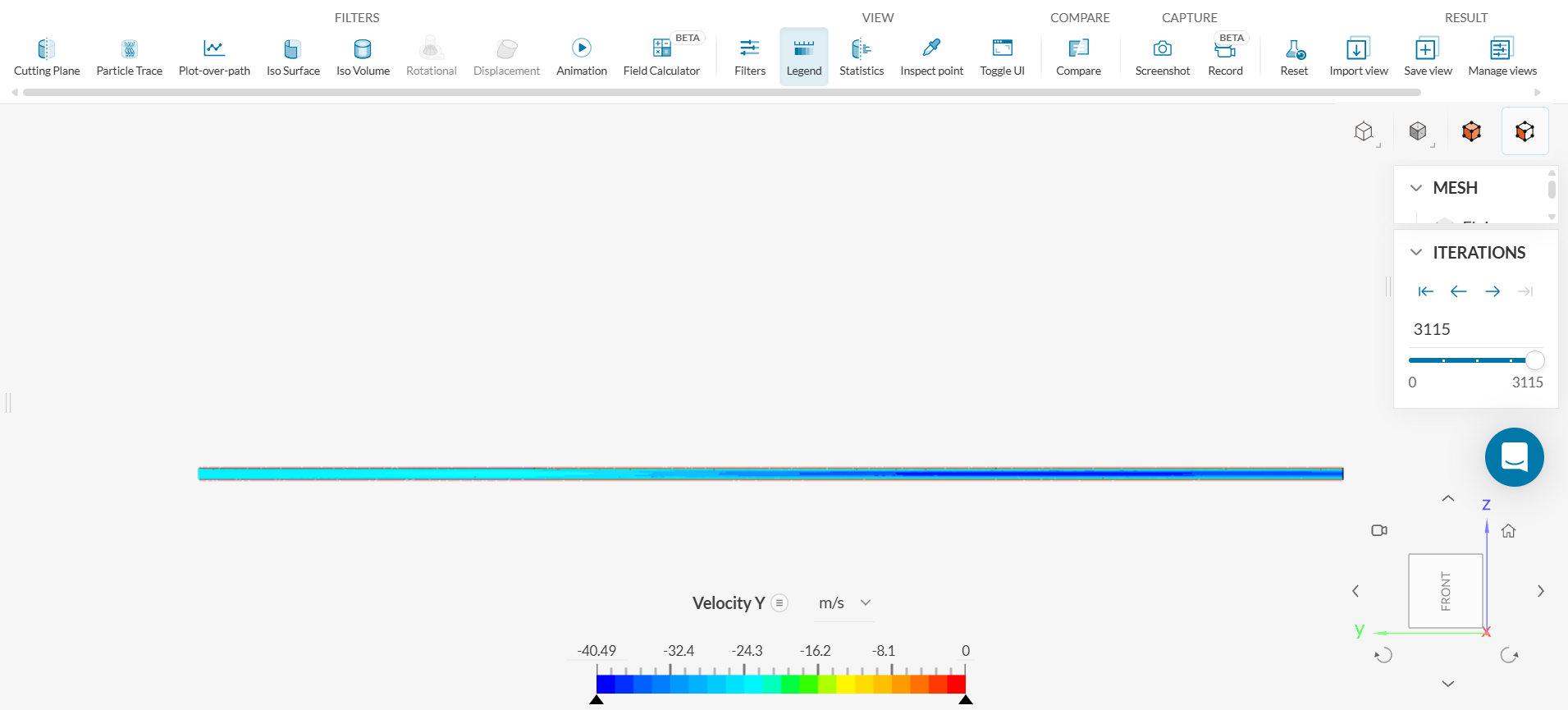
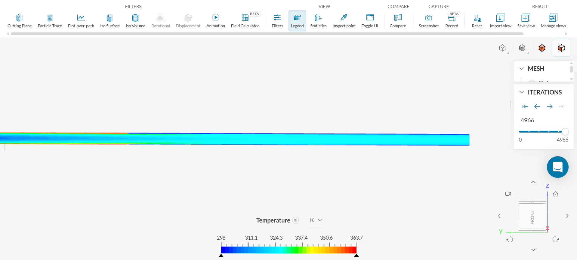
5.2 Velocity Contours

Click on the three bars next to ‘Temperature’ on the legend located on the bottom of the screen and click on ‘Velocity - Y’ to view the velocity contour. The figure below shows the y-velocity throughout the length of the pipe.

The velocity contour shows that a boundary layer starts to form throughout the pipe. In the heated section of the pipe, the velocity increases in magnitude. This is dictated by the conservation of mass. As the pipe is heated, the flow is faster because the density of air decreases with increasing temperature. To keep the mass flow rate constant, then, the velocity must increase.

A comparison of the velocity profiles in the flow development and fully developed region will be given after a mesh refinement.

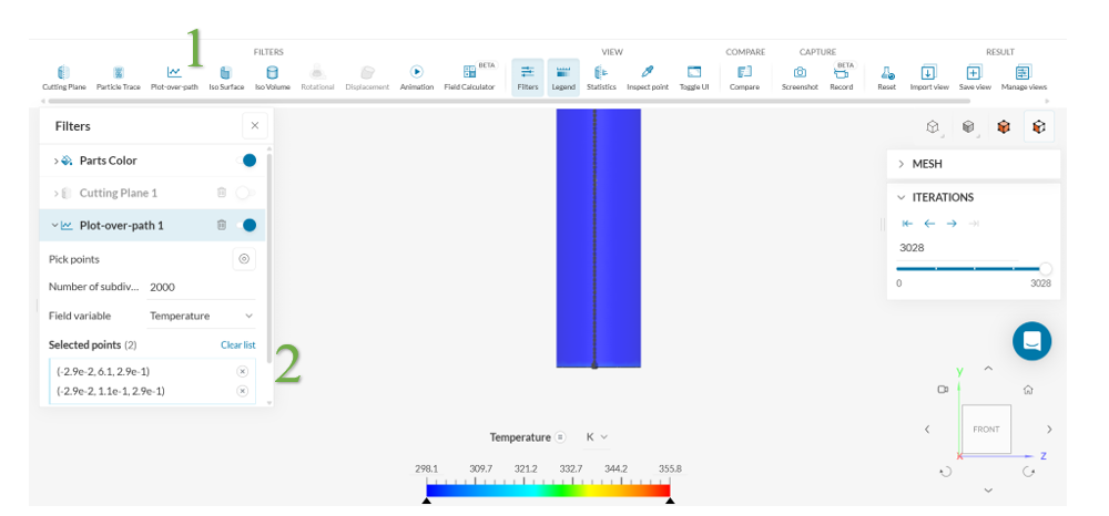
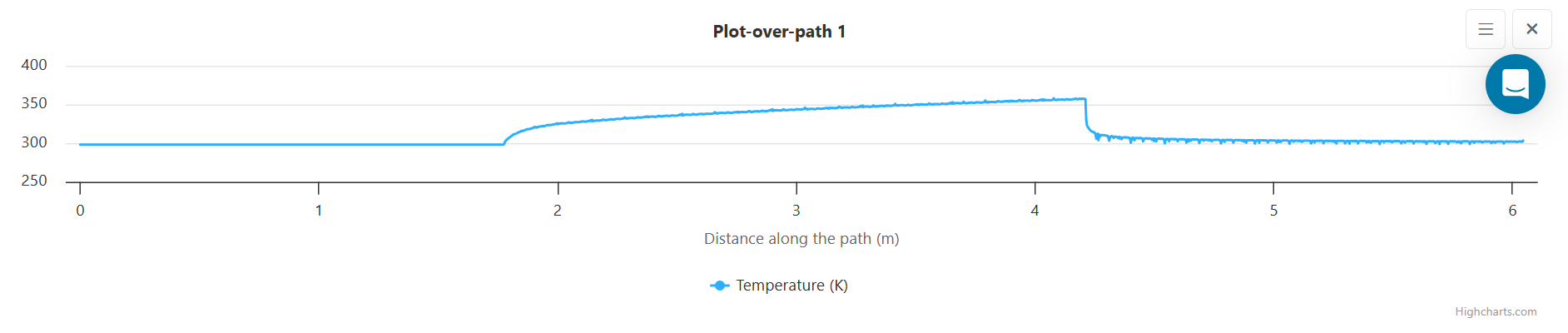
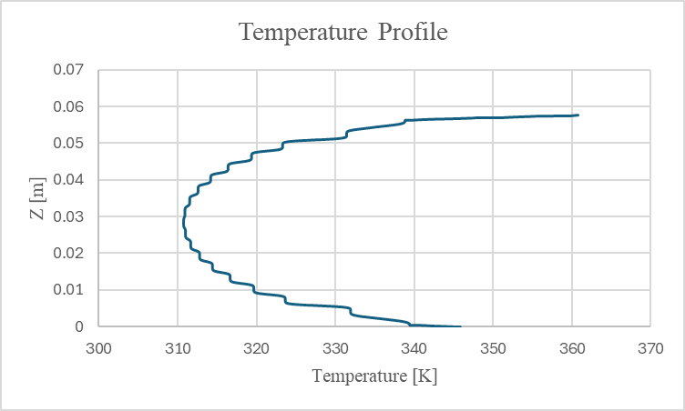
5.3 Wall Temperature Plot

The Wall Temperature plot shows the change in temperature along the wall of the pipe. To generate this plot,

1. Hide the ‘Cutting Plane 1’ by turning off the adjacent toggle located on the right side of the Filters panel.

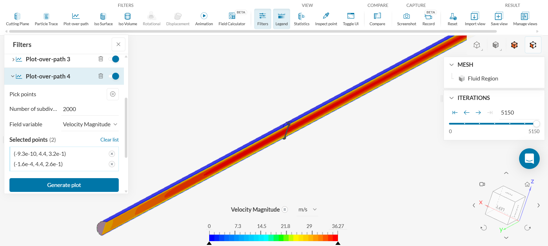
2. Click on ‘FILTERS: Plot-over-path.’

3. Select two points along the wall of the pipe. With the global coordinates showing the ‘Front’ View of the pipe, the first point to pick should be at the top of the pipe and the second point should be at the bottom of the pipe.

4. Type 2000 for the ‘Number of subdivisions’

5. Choose ‘Temperature’ for the ‘Field Variable’

6. Click ‘Generate plot’

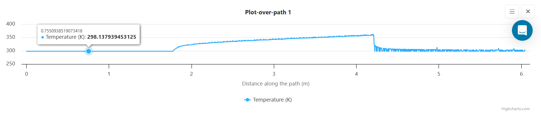
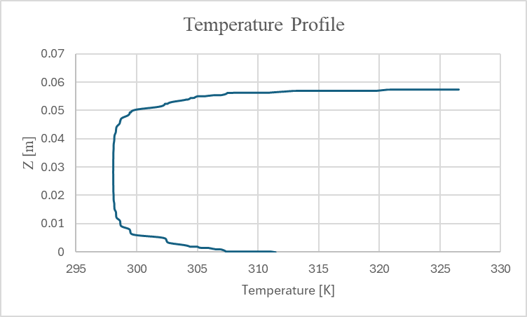
The plot of temperature along the y-axis and distance along the pipe along the x-axis is shown below:

The first section of the pipe is not heated and shows the initial temperature of 298.15 K. The heated section of the pipe is from 1.83 m to 4.27 m. The temperature along that line shows a temperature increase. In the third section, where there is adiabatic mixing, there is nearly uniform temperature.

5.4 Verification and Validation Checklist

5.4.1 Check the Boundary Conditions and Conservation of Mass

While in the post-processing, the boundary conditions should be checked as part of the verification process.

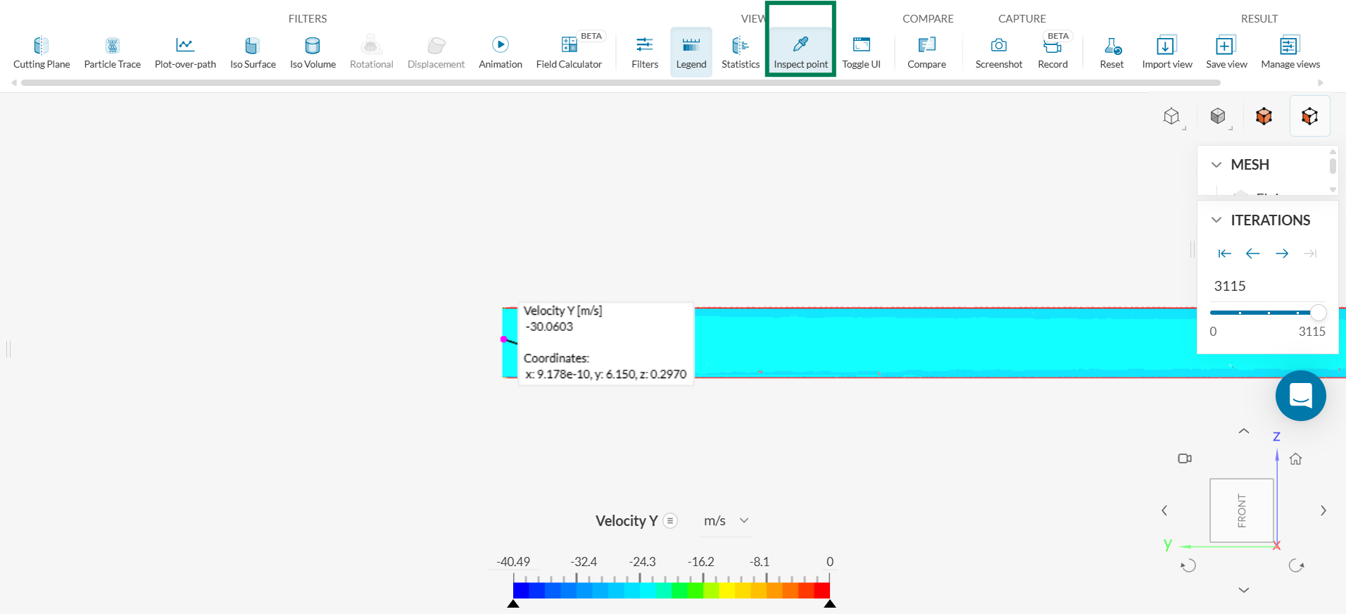
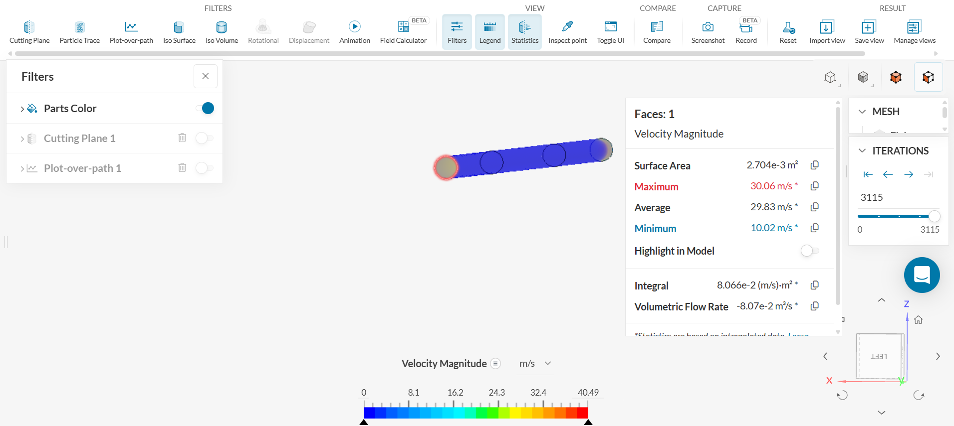
1. Check to see that the velocity at the inlet is -30.06 m/s. Click on ‘VIEW - Inspect point’ and click on the left side of the pipe (or the side of the inlet of the pipe)

The velocity in the y-direction at the inlet is shown to be -30.0603m/s.

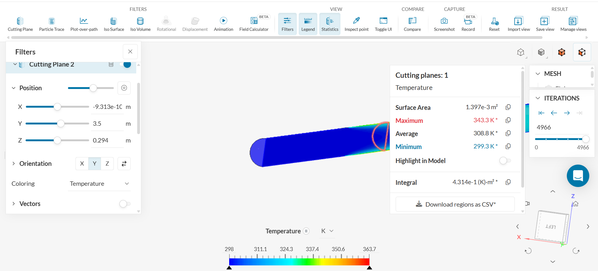
2. Compare the volumetric flow rate at the inlet, center, and outlet of the pipe to verify the conservation of mass.

i. Click on the inlet face and then click on ‘VIEW – Statistics’ to check the volumetric flow rate.

The volumetric flow rate is -0.0807 m^3/s at the inlet.

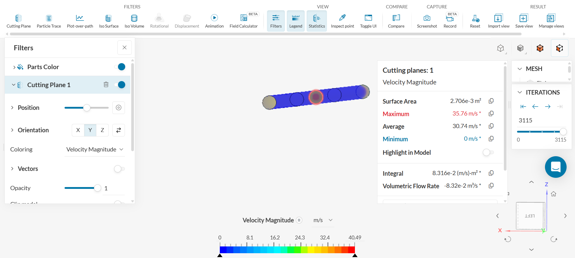
ii. Click on ‘FILTERS – Cutting Plane’ and choose ‘Orientation – Y.’ Do not clip model. The face will be highlighted at the center of the pipe. The volumetric flow rate is -0.0832 m^3/s

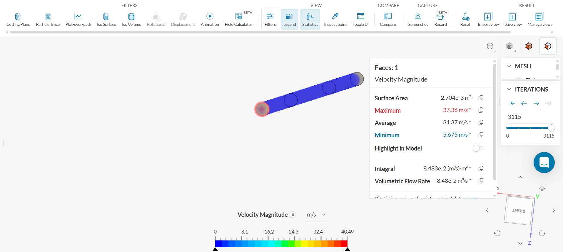
iii. Click on the outlet face and then click on ‘VIEW – Statistics’ to check the volumetric flow rate.

At the outlet, the volumetric flow rate is 0.0848 m^3/s.

The volumetric flow rate increases at the center and outlet because the temperature increases at those locations. When temperature increases, density decreases and the volumetric flow rate (or velocity) must increase to obey the fulfill the conservation of mass. Check the densities at inlet and outlet.

Find the average densities at the outlet and inlets by click on the three bars next to Velocity Magnitude Legend at the bottom of the screen and selecting ‘Density’.

At the outlet, the average density is 1.092kg/m^3. Thus, the mass flow rate at the outlet is 0.0926 kg/s. At the inlet, the average density is 1.149kg/m^3. The mass flow rate at the inlet is 0.0927kg/s. The percent difference is 0.108%.

5.4. 2 Linearization Error

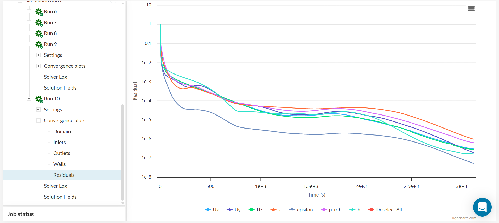
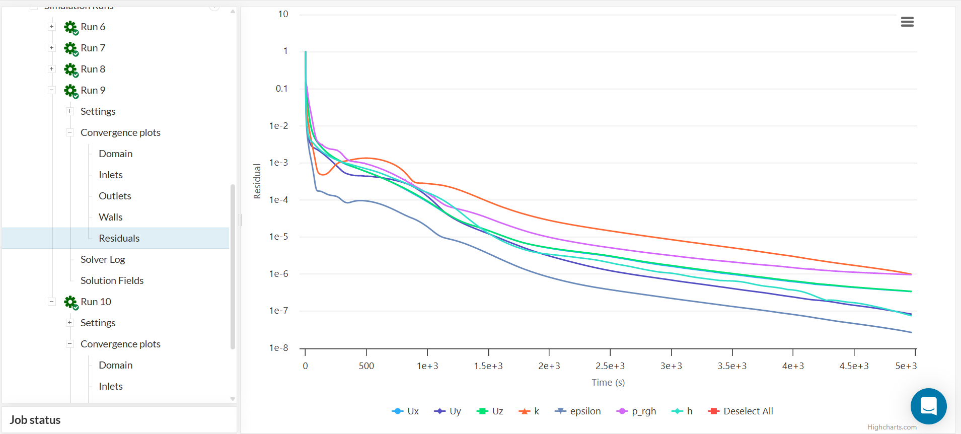
Check the linearization error by navigating to ‘Convergence plots – Residuals.’ Verify that the residuals are below the set tolerance of 1e-6.

5.4.3 Discretization Error

Check the discretization error by refining the mesh and check if the result improves. Change the mesh to a ‘Fineness’ of 7 instead of 6. This will generate 2.7 million cells and 1.2 million nodes, almost double the cells generated in the previous mesh.

Check the linearization error by navigating to ‘Convergence plots – Residuals.’ Verify that the residuals are below the set tolerance of 1e-6.

Temperature Contour over Refined Mesh

Check the temperature contour and the plot of the temperature along the wall. Does it give a more uniform temperature along the adiabatic mixing region?

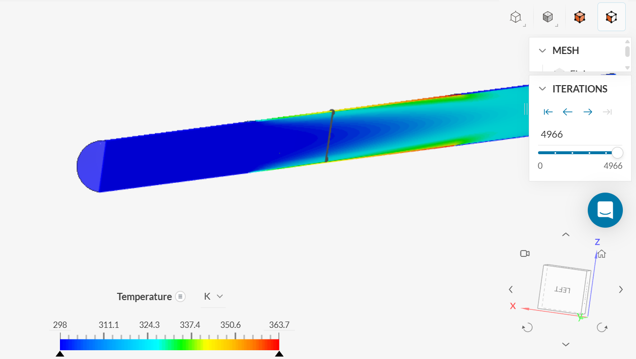
Velocity Contour over Refined Mesh

View the Velocity Contour. A boundary layer starts to form along the pipe.

The hydrodynamic entrance length, over which the flow becomes fully developed is given by

and the Reynolds number is given by

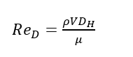
where the numerator is the product of the density, inlet velocity and diameter of circular pipe (hydraulic diameter) and the denominator is the dynamic viscosity.

The result of the hydrodynamic entrance length is 1.7908 m.

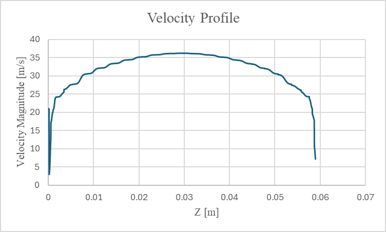
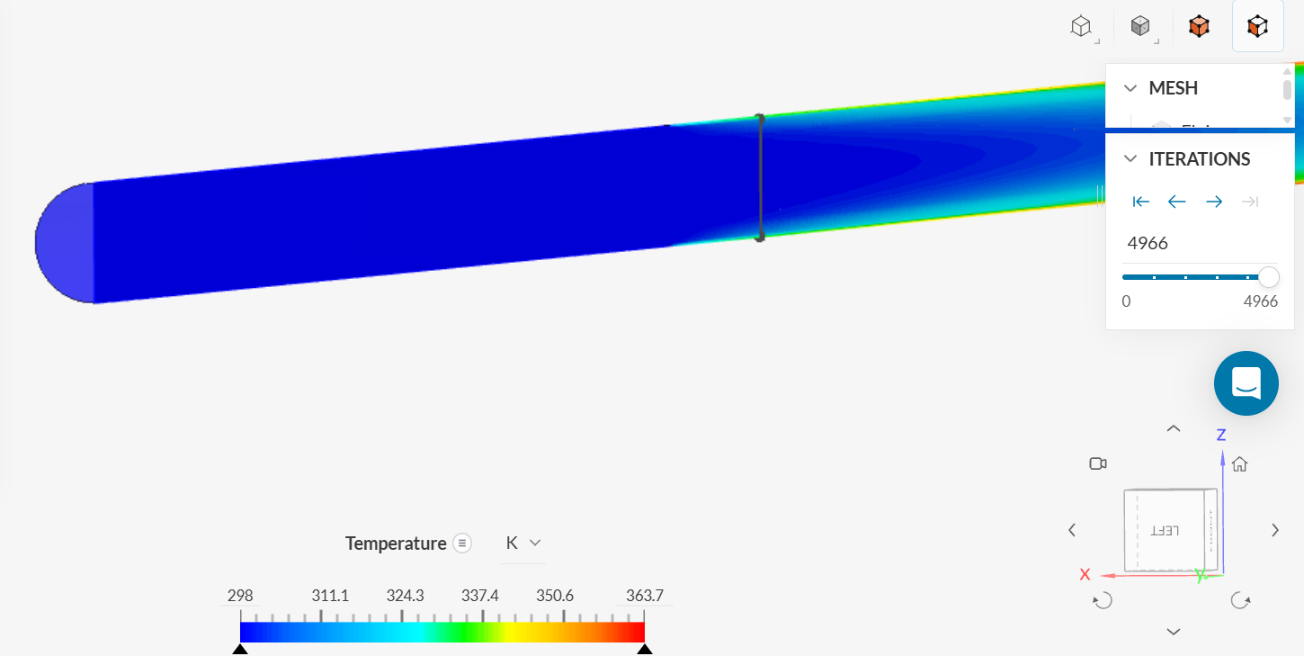
To plot the velocity profile at a line, use the ‘FILTERS: Plot-over-path.’ An example is shown below:

The velocity profile at around y = 1.7908 is shown below:

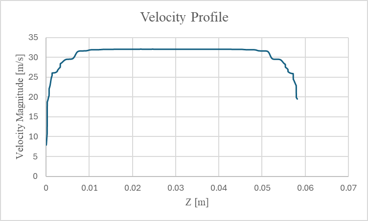
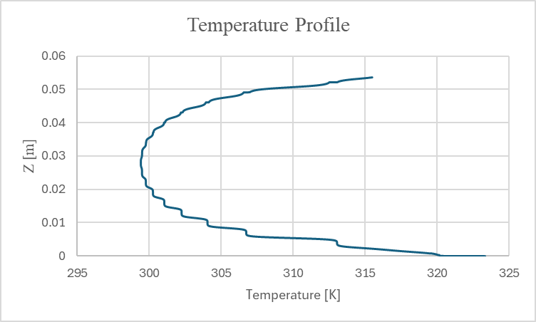
In comparison, the velocity profile at the start of the pipe at 0.351 m is shown below:

The velocity profile at around 1.7908 m appears more developed.

Note that the refined mesh shows the expected velocity profile. The refined mesh should be used for further calculations.

Nusselt Number

The Nusselt Number can be calculated from the SimScale Post-Processing results and can be compared to the theoretical value.

The value for the Nusselt Number derived from a forced convection in turbulent pipe flow can be calculated from Gnielinski correlation.

Gnielinski’s correlation for flow in tubes is used with 3000≤Re_D≤5×10^6. The Gnielinski’s correlation for the Nusselt Number Nu_D is given by

where f is the Darcy friction factor that can be evaluated from correlation developed by Petukhov for smooth tubes:

1. The first step is the calculate the Reynolds number. Use the equation for Reynolds number provided above.
2. Calculate f
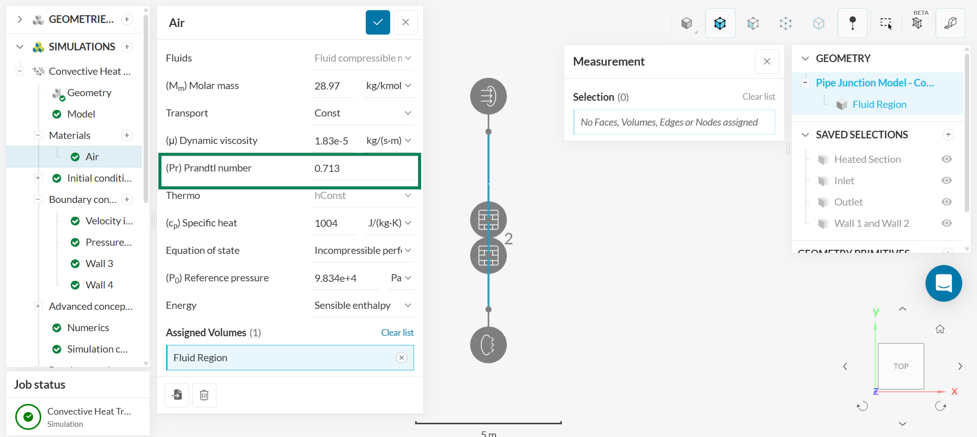
3. To find the Prandtl number, navigate to ‘Materials - Air’ in the SimScale Simulation tree to locate the Prandtl number:

The Nusselt number from the Gnielinski’s correlation is calculated to be 196.114.

The Nusselt number from the SimScale Post-Processor can be calculated by following the steps below.

1. Use the equation 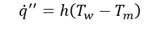to find the heat transfer coefficient h. The heat transfer coefficient can then be normalized to find the Nusselt number.
2. T_m represents the mixed mean temperature. The mixed mean temperature represents the overall heat transported by fluid through a cross section of pipe. From the energy equation, the mixed mean temperature varies linearly in the heated section of the pipe. Thus, the mixed mean temperature T_m can then be calculated from the slope of the line between the flow development region and the adiabatic mixing region. To find T_m:

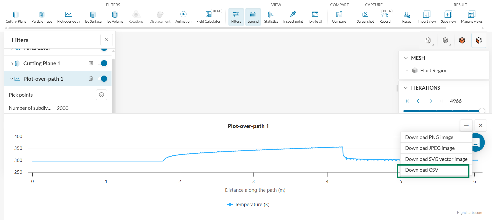
• Plot the Wall temperature along the pipe using the directions from the Section Wall Temperature above.

• Download the plot as a CSV file and plot Wall temperature over the length of the pipe in Microsoft Excel.

  
  

The region of fully developed heat transfer occurs when the difference between T_w and T_m stays constant. An approximate value is shown on the above plot.

• Since the mixed mean temperature is constant in the flow development region, pick a point that coincides with the temperature along Flow Development region (298.15 K) and 1.83 m (the start of the heated section). Since the mixed mean temperature is also constant along the adiabatic mixing region, pick another point that coincides with the temperature along Adiabatic Mixing region and 4.27 m (the end of the heated section). Insert a trendline and display the slope of the trendline on the graph.

• Find the region where the flow is thermally fully developed by using the ‘View - Inspect’ point on the temperature contour plot in the SimScale Post-Processor.

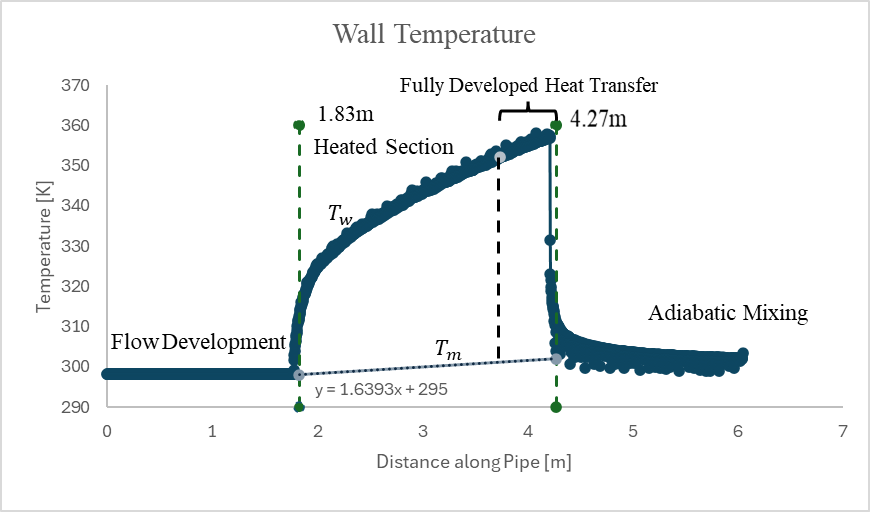
The expected thermal entrance length is at 2.418 m from the start of the pipe approximately. This translates to the y-coordinate y = 3.733. As a check, here are the temperature profiles at different lines along the pipe.

y = 3.7 or line at approximately 2.45 m from start of pipe:

y = 4.1 or line at approximately 2.051m from start of pipe:

y = 3.5 or line at 2.651 m from start of pipe:

y = 1.97 or line at approximately 4.181 m from start of pipe:

First, the mixed mean temperature will be calculated at coordinate y = 3.5 or a distance of 2.651 m from the start of the pipe. The mixed mean temperature is 302.5 K.

• To find T_w at the coordinate y = 3.5m, use the ‘Cutting Plane’ and find the maximum temperature value by using the ‘VIEW - Statistics’ feature.

In the equation , q’’ is 5210.85 W/m^2 and T_w is 343.3K and T_m is 302.49K. Solve for the heat transfer coefficient, h. The heat transfer coefficient is 127.69W/m^2 K.

The heat transfer coefficient should be constant throughout the thermally fully developed region. Repeat the above calculation at a different axial location in the heated section— at y = 1.97, for example. This location is chosen because from the graph of the Wall temperature vs length of the pipe, the difference between T_w and T_m remains approximately constant. Also, the temperature profile shows to be more developed at that line. Find T_w and T_m at coordinate y =1.97 by following the steps above. The heat transfer coefficient at y = 1.97 is 88.779 W/m^2 K. The heat transfer coefficient at y = 2.3 is 93.996 compared to the heat transfer coefficient at y = 1.97 m where the heat transfer coefficient is 88.779 W/m^2 K. The percent difference is about 5.7%.

The Nusselt number will be calculated from the heat transfer coefficient of 88.779 W/m^2 K. Normalize h by the following equation: 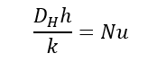where D_H is the hydraulic diameter and k is the thermal conductivity to get the Nusselt number. The thermal conductivity k = 0.0266 W/(m K).

The Nusselt number calculated from SimScale is 196.24.

The percent error is about 0.0687%.

Further Checks

1. Plot the Temperature profile at the start and end of the heated section and check if there is a temperature increase.
2. Refine the mesh to see if the results improve.
3. To further check the results, change k and or the Turbulent Intensity % and the Turbulent Viscosity ratio to confirm the results do not significantly change.