Dear fellows,
In this project, I have performed a cooling study of a small house using transient analysis approach (Unsteady RANS). There is one airflow inlet and one exhaust/outflow. The walls of the house are treated as adiabatic wall for the sake of simplicity. The initial temperature inside the house is 85 °F while the airflow entering the house is 60 °F. I have tested the airflow entering the house at +45° and -45° angles. Temperature profiles at various points are plotted for initial 30 minutes in +45° case and for initial 15 minutes in -45° case. Adjustable time step is used in the simulation control. The animations provided are generated using ParaView.
This project focuses on the study of small home cooling and the airflow patterns inside the home. Transient (convective) heat transfer analysis is used to model the evolution of temperature in the home over time.
1. CAD Geometry
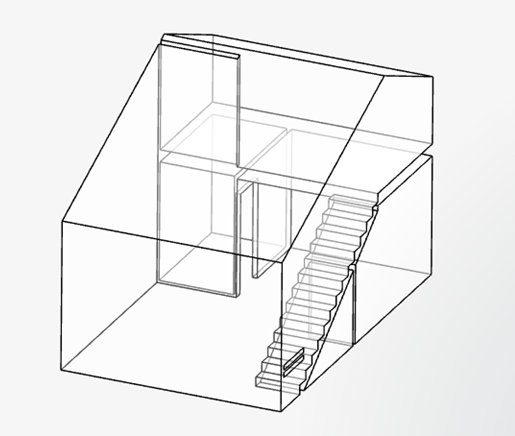
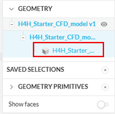
CAD geometry was prepared, cleaned in the local machine, and uploaded to the SimScale platform.
You can download the geometry “H4H_Starter_CFD_model v1” to upload it later to your newly created project.
Login to the SimScale, copy the project
OR
Login to The SimScale, create a new project, and upload the geometry you have downloaded earlier. Whole geometry is created as a single solid volume with various surfaces.
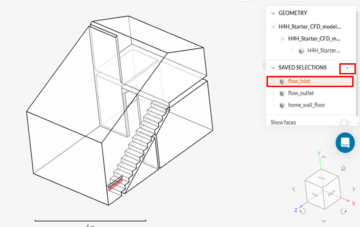
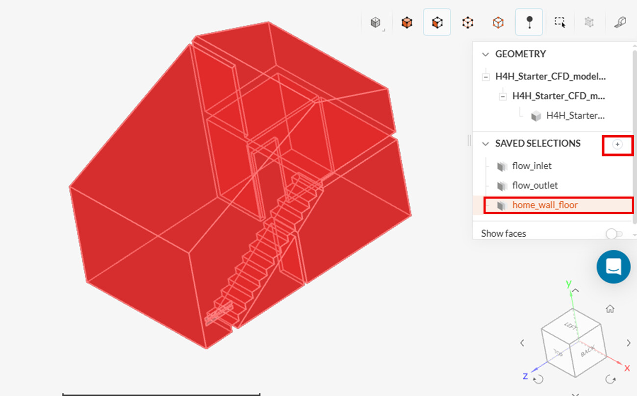
Create and save selections for ease of work and later use.
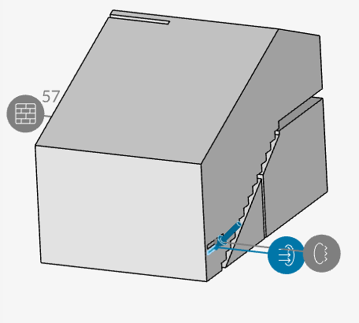
First create selection for inlet face and rename it to flow_inlet.
Then create for outlet face and rename it to flow_outlet.
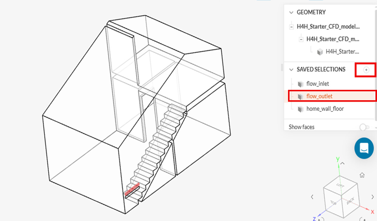
The last selection includes all faces except inlet and outlet faces.
2. Simulation Setup
2.1 Create Simulation
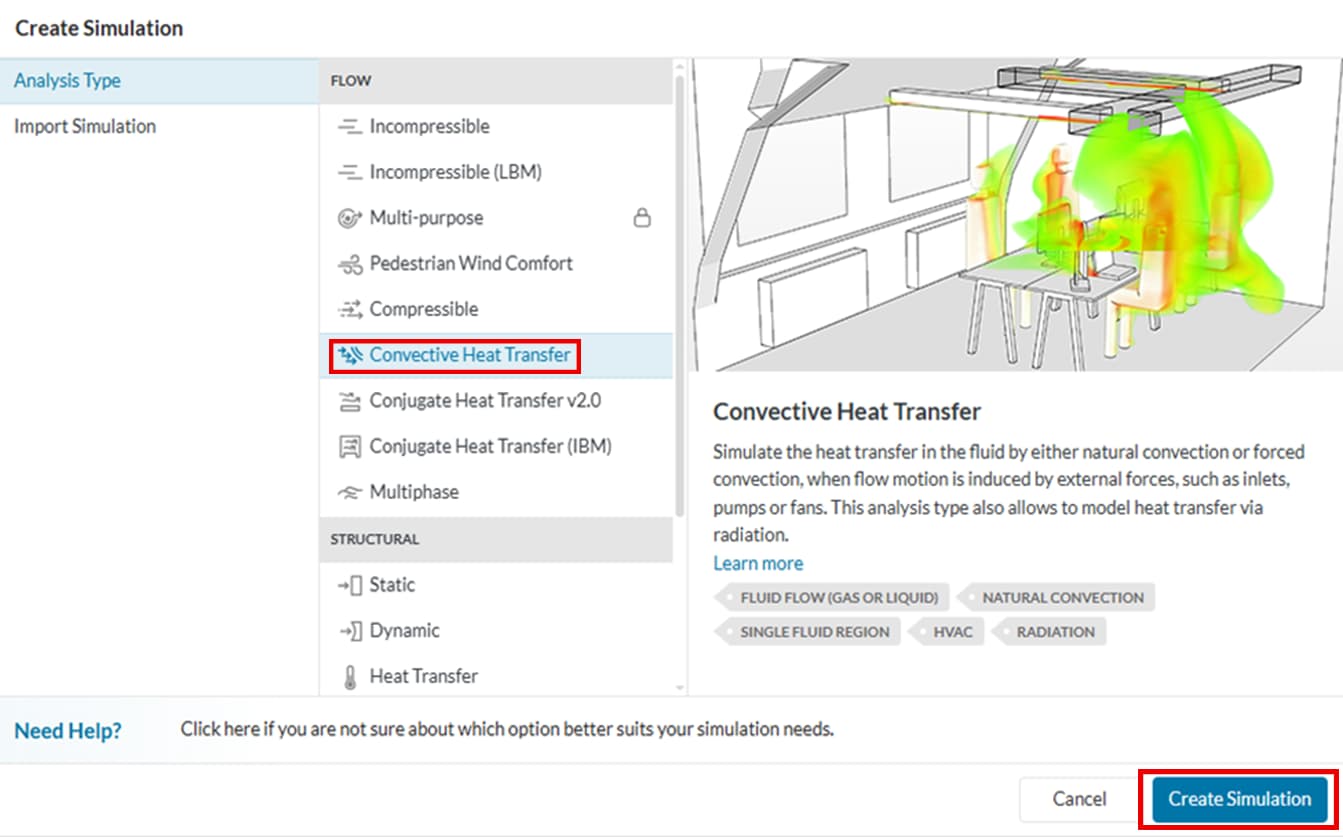
With geometry “H4H_Starter_CFD_model v1” selected, click “Create Simulation”.
Choose “Convective Heat Transfer”. We are interested in the convective heat transfer study inside the home as the cold air is being supplied.
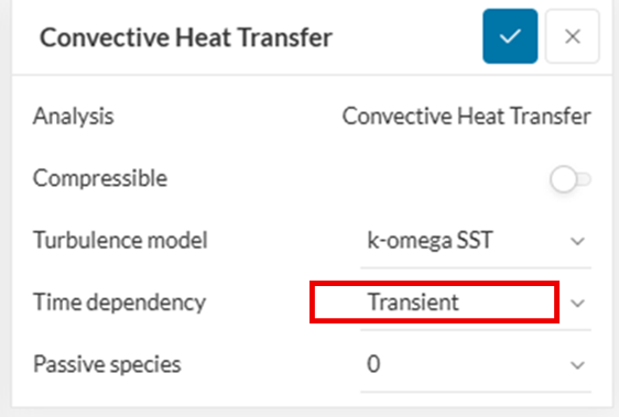
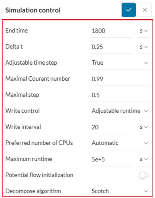
We are using the Convective Heat Transfer study with Time dependency as “Transient” because we are interested in the evolution of temperature (home cooling) over 30 minutes (1800 seconds) duration.
2.2 Add Geometry Primitives
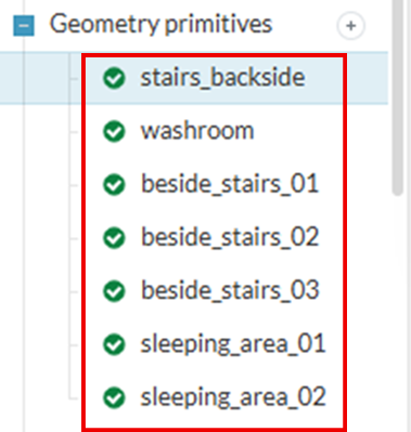
We have added 7 geometry primitives (point coordinates) here to track the evolution of temperature later.


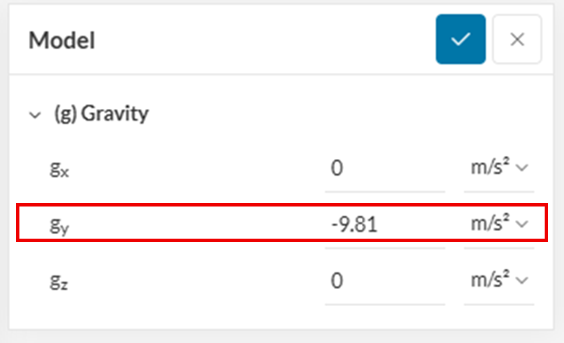
2.3 Gravity
Add gravity to the model
2.4 Material Assignment
Assign “Air” as a material.
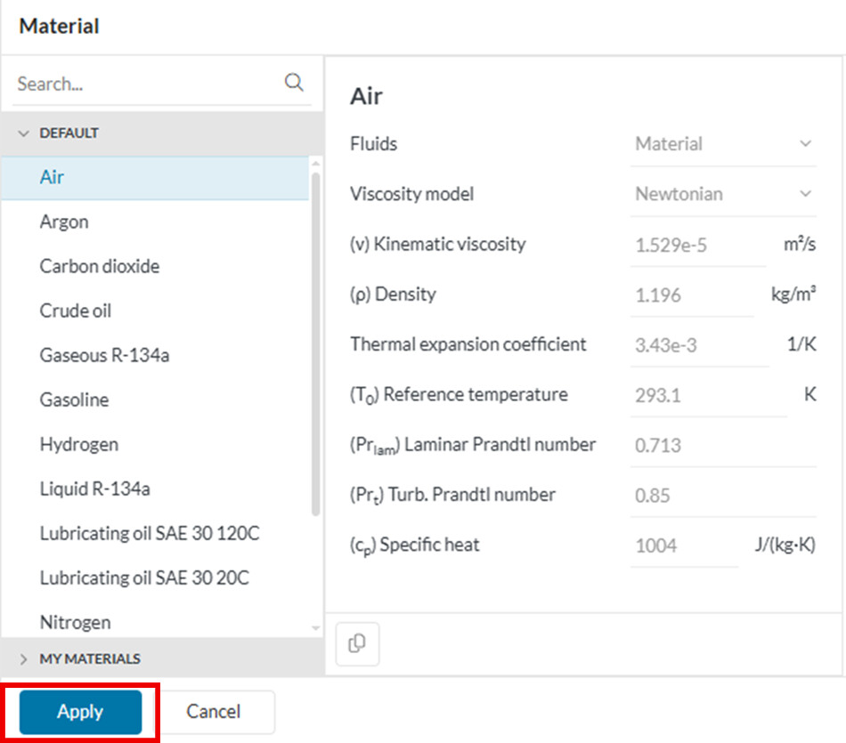
Then assign “H4H_Starter_Home” as the volume in the material volume assignment.
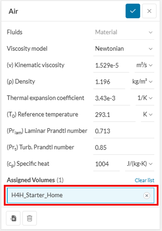
Click “Save” after assignment.
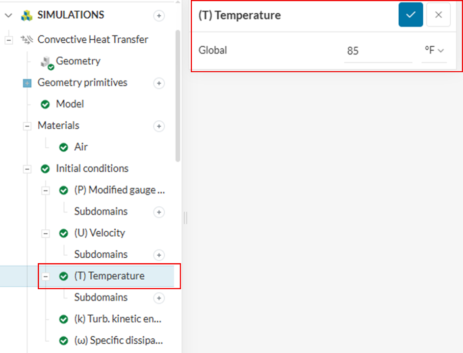
2.5 Initial Conditions
Put initial velocity Uy = 0.01 m/s and keep the Ux and Uz as 0.

Put initial temperature (T) Global as 85 °F.
2.6 Boundary Conditions (BC)
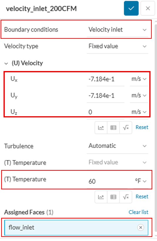
2.6.1 Velocity Inlet
Assign the velocity inlet boundary condition to the flow_inlet face. We will use the flow velocity corresponding to the 200 Cubic Feet Per minute (CFM) flow rate at -45° angle. This corresponds to -0.71842049 m/sec in each x and y directions.
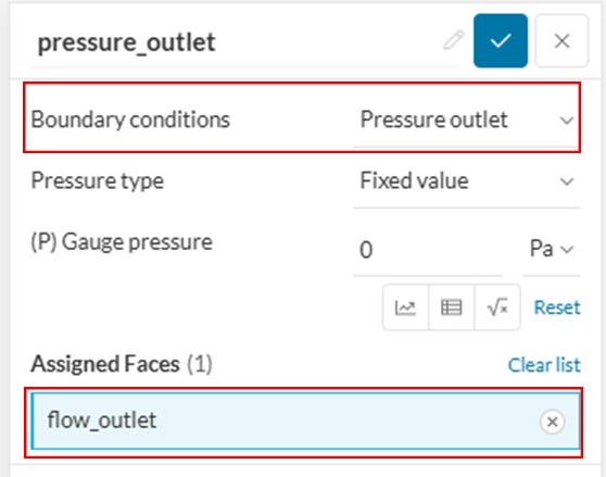
2.6.2 Pressure Outlet
Assign the pressure outlet BC on the “flow_outlet” face.
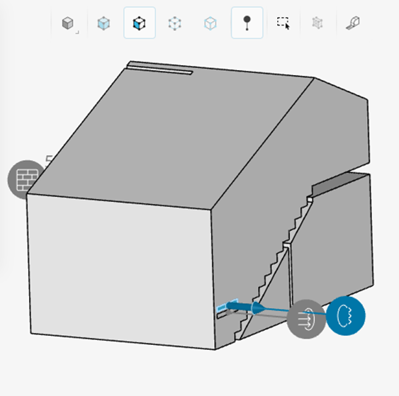
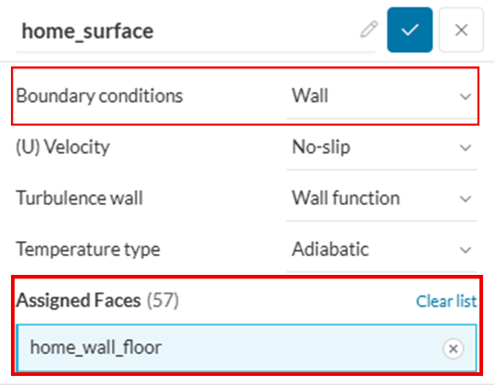
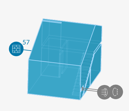
2.6.3 Wall
Assign the “No-slip” wall BC on all faces (except inlet and outlet faces).
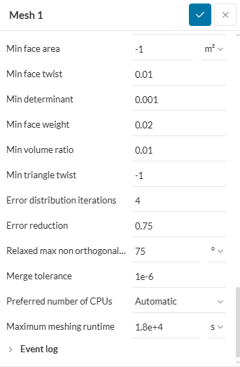
3. Mesh Generation
3.1 Mesh Selection
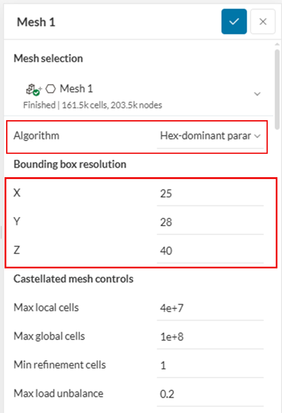
In this simulation, we are using “Hex-dominant parametric” algorithm to generate a high-quality mesh suitable for our case.
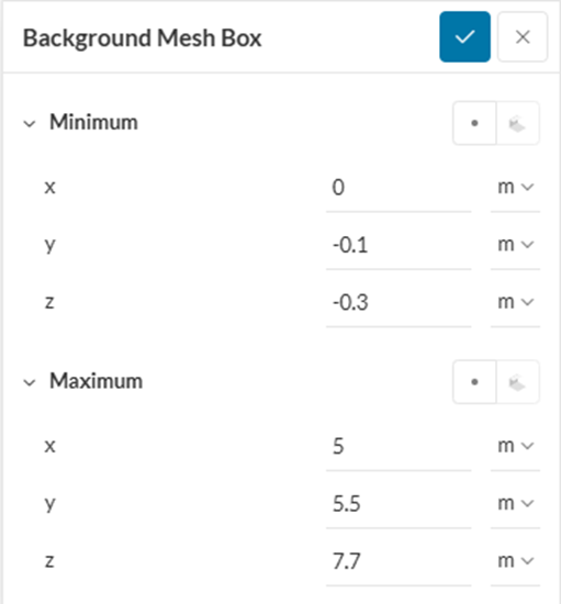
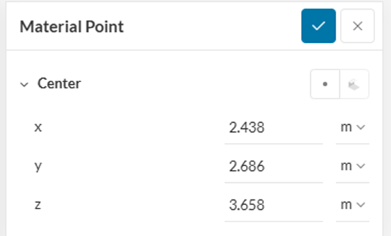
3.2 Geometry primitives
Set the dimensions of the background mesh box as mentioned below:
Put the material point according to the coordinates below. It must be inside the fluid domain.
3.3 Refinements
Assign surface refinements of level of min 3 and max 4 to the inlet and outlet faces.

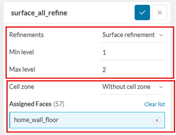
Assign surface refinements of level min 1 and max 2 to the walls and floor faces.
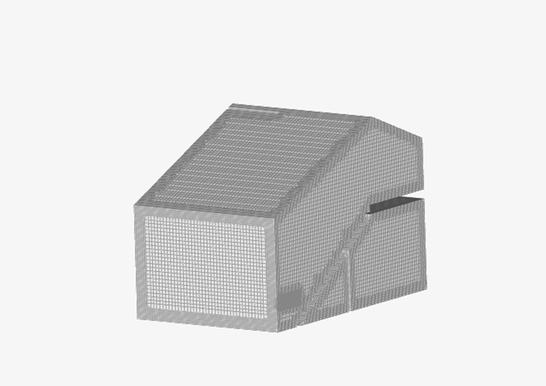
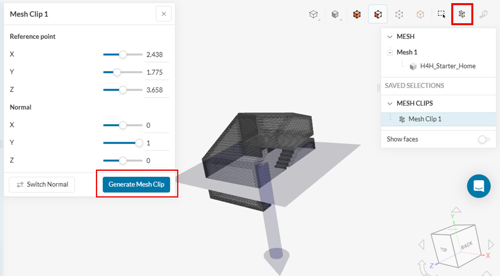
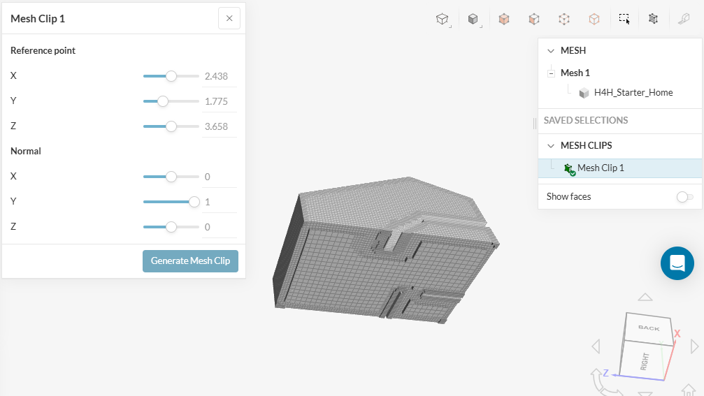
Generate the mesh. After mesh generation, preview the mesh. You can view the inside of the mesh using “mesh clip” feature.
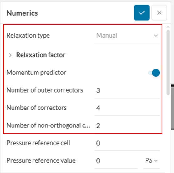
4. Numerics
Set the correctors as shown in the image below:
5. Simulation Controls
In one case, we are simulating the flow at +45°, while in another case we are simulating the flow at -45°. We are looking for 30 minutes of airflow inside the home, which corresponds to 1800 seconds. We are using adjustable timestep settings with maximum courant number limit of 0.99.
6. Result Control
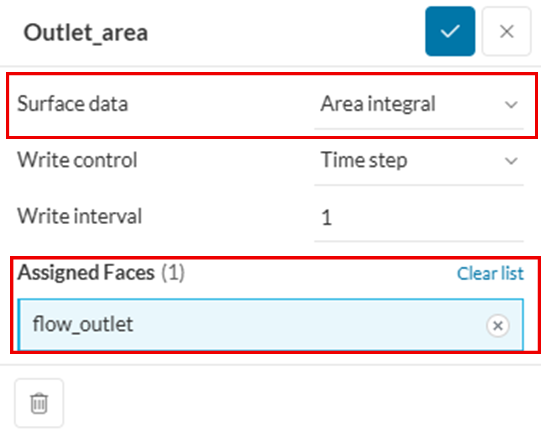
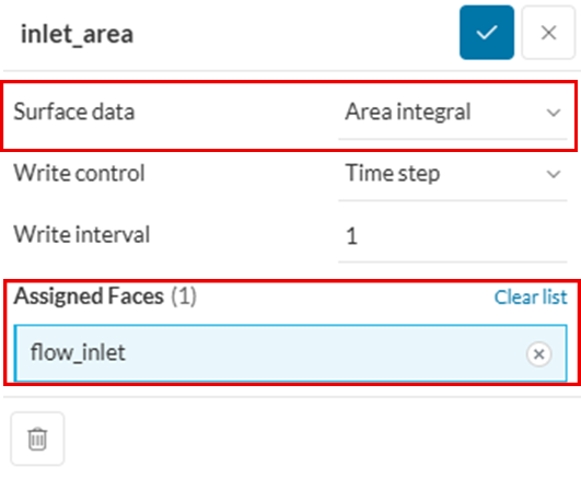
6.1 Surface Data
In result control section, first go to “Surface data”.
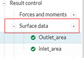
Choose Surface data as “Area integral” and assign an outlet face (flow_outlet in our case).
Once again, choose Surface data as “Area integral” and assign an inlet face (flow_inlet in our case).
6.2 Probe Points
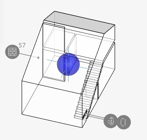
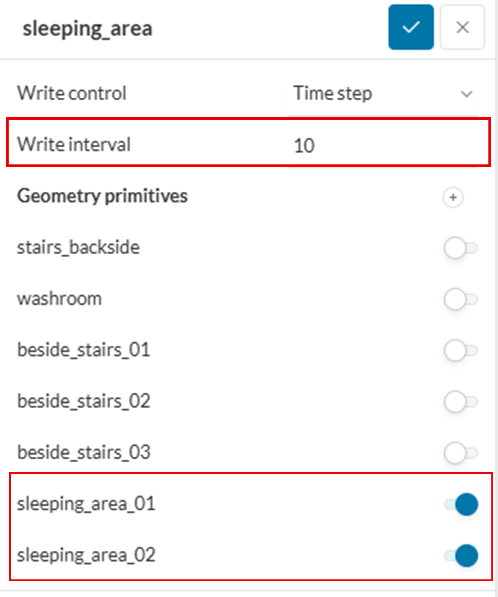
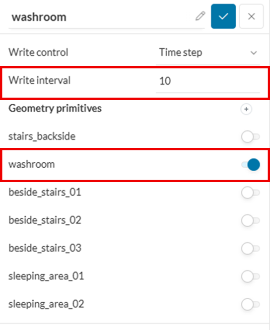
Now, go to the “Probe points” and create 4 different probe points.
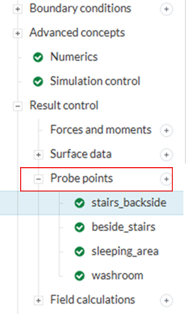
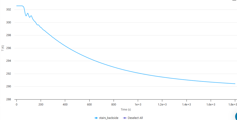
In our case, first primitive is on the back side of the stairs. Add it as a probe point as below.

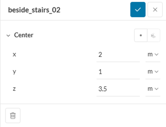
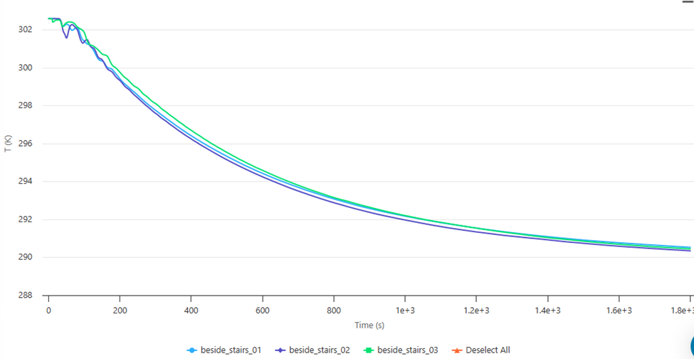
Choose primitives beside the stairs altogether and add them to one probe as shown below.

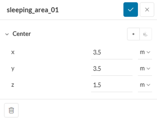
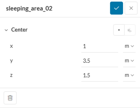
Choose primitives in the upper floor and add them to one probe as shown below.
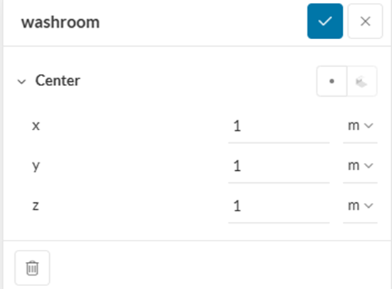
Choose geometry primitive in the bathroom/washroom and add it as probe point.
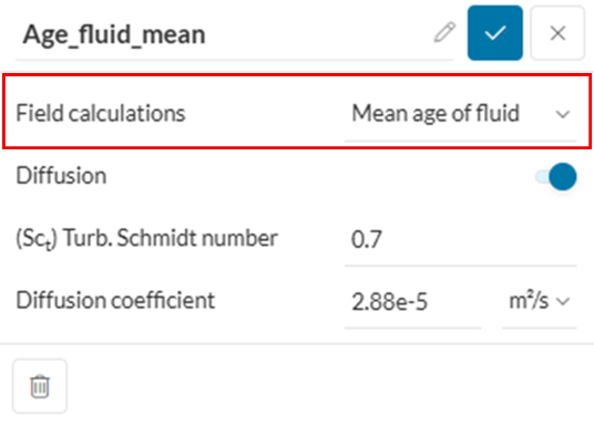
6.3 Field Calculations
Finally, in the “Field calculations”, select “Mean age of fluid”.
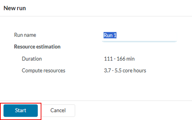
7. Simulation Runs
In the “Simulation Runs”, create a “new run”, rename it as per your choice, and click “Start”.
8. Post-Processing
8.1 Probe Point Plots
Check evolution of temperature at specified probe points during and after the simulation.

In the “Probe point plots”, go to sleeping_area and select temperature (T)

You will be able to see a plot like this.

Repeat the same procedure to check other plots.

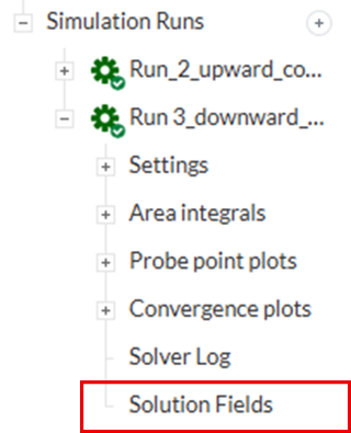
8.2 Solution Fields
You can visualize the contours of different variables in the solution fields.
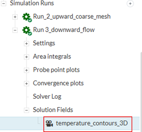
For example, you can check the temperature variation with time using “Animation” filter and save the animation using “Record” feature in post-processor.
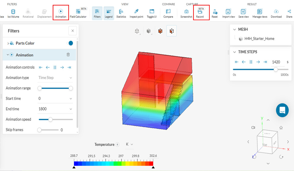
Animation is also saved for reference.
The other animations shown in the post were plotted using ParaView.