To capture the mesh better around sharp edges

[vishnu_1000]

I am working on a simple case of a laminar flow around an airfoil. Following are the specifications:
Flat Plate :
Length =100mm=0.1m
Thickness(ideally infinitesimally thin), here 1mm
Flow:
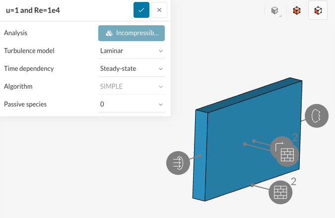
u=1 m/s, kinematic visc =1e-5, density =1 kg/m^3, thus Re=1e4

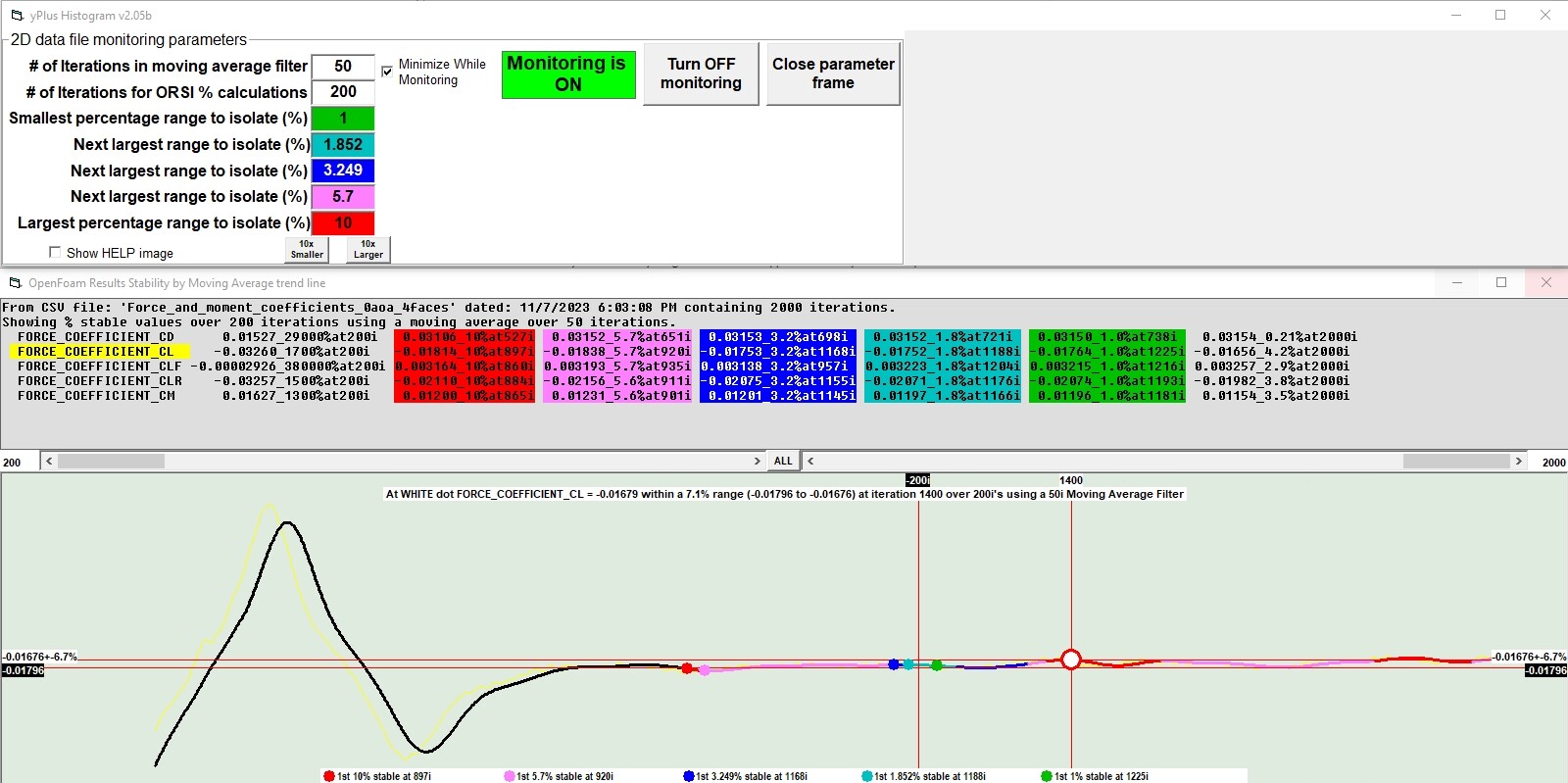
I am trying to calculate the value of drag coefficient whose expected value if 0.0138, whereas I’m getting a simulated value of 0.019, which is larger than expected. I believe this is likely because of ratio of thickness:length is supposed to be even smaller, and I am going to try with even smaller thickness. However, one other possible reason for wrong error is the skewness in the mesh as it it isnt capturing the thickness edge properly. I am using hex dominant mesh for creating the mesh.

For any further details/ simulation set up, following the link to my project(test): https://www.simscale.com/workbench/?pid=8986269944862089602&mi=spec%3A45b1afc6-b77c-42e2-8d56-cdb7d2fa41f9%2Cservice%3ASIMULATION%2Cstrategy%3A38

The above image only shows only one face, as it is a 3D case implemented with symmetry BC on both sides to make it 2D, the skewness goes all along the thickness edge.

Even if I am using another CAD model with even smaller thickness, I am sure that I will encounter the same problem. It would be great for someone to tell me what could be done?

Thanks,
Vishnu

[DaleKramer]

So far on a cursory look:

1. I can see that you are not defining any boundary layers.
2. Your refinement areas are outside your boundary box so no mesh refinements are made inside them:
   
   

[vishnu_1000]

Also, I tried creating a cad model of 0.001 mm thickness, and of the same length. However, while creating the domain for the same, there is a step where we delete the solid to get the flow region alone. However, while deleting, it is giving one whole domain alone, which I believe is because of too small a thickness which I have tried to use.

[vishnu_1000]

Oops thanks for the region refinement part.
Also, the boundary conditions have been defined for the main domain. Take a look at the following:

[DaleKramer]

But the mesh that you linked to was ‘T1 mesh’, which does not have an ‘Inflate boundary layer’ refinement which creates actual prism cells for the boundary layers…

I think your mesh only contains hex cells.

[DaleKramer]

Also, it seems that you want to do a Validation assessment which determines if the computational simulation agrees with physical reality.

Be very careful that you do not adjust your Meshing , CFD simulation setup and parameters until you obtain the coefficients that you see in reality. But rather try to obtain the best CFD results you can achieve using best practices to achieve them.

I spent a LOT of time trying to validate the NACA0012 airfoil years ago and was never able to use best CFD practices that matched real world results. I never achieved CFD results that were even close.

In my opinion, the CFD validations that I looked at, where people came close to reality, could not be justified as blindly using best practices. This is especially true where you expect low drag coefficients.

[vishnu_1000]

Hey Dale!!

Firstly, thanks a ton for your valuable input. I found the careless errors that I had made in the simulation setup, which I have now fixed.

Expected Cd= 0.0138
Simulated Cd = 0.0119
Error % = 13%.

Please take a look at the present set up :

SimScale Login

However, I am getting a value for Cl be negative -0.02, when it is actually supposed to be 0. Are these values of Cd and Cl considered okay or is there anything which I am still supposed to rectify in the set up ?

[DaleKramer]

Hi,

I have seen this years ago in my NACA0012 analysis. I suspected then that the randomness of turbulence handling was the issue.

And your current CL < 0 issue has influenced me enough to have another look at studying the NACA0012 at 0 degrees AOA using the current version of the Standard Mesh Algorithm that auto generates boundary layers.

So I started with a project setup from back then and I have not exhaustively determined that I have used current best practices on the results I will show you now but it does seem to match your results.

I used yPlusHistogram to determine that the overall yPlus was acceptable to use for the log-log region and got this (I am a little concerned about the 4.3% of the total cells below a value of 15) :

.
.

Then I analyzed the convergence stability of the Coefficients using the ORSI feature of yPlusHistogram and got this output that shows the yellow CL results plotted in the image:

The Yellow plotted line is the actual results from a downloaded csv file of SimScales results.

The multi color line is the moving average of the actual results using the moving average parameters shown at the top.

The colors of the multicolor line show where the moving average plot is stable over the number of iterations and color ranging specified at the top of the image.

My conclusion from looking at this ORSI analysis is that the CL stability is not highly stable. I like to see a continuous GREEN line of a few hundred iterations in length (<1% data variation) at the last iteration of the plot. We did hit green at one point, but only for a short time.

In any case of stability analysis we can only say the results are stable to only about 5%, which is OK in some peoples books for certain applications. The ‘sorta 5%’ stable values run from -.017 to -.018 which seems intuitively incorrect and matches your experience with your flat plate analysis.

So, this issue still exists, as it did over 3 years ago.

I still think it has to do with how turbulence is handled in the code which generates these results.

I hope a more learned scholar on this issue can jump in here and ‘shed some light’ on the situation