Our aim is to analyse the sliding of a rubber seal on a rigid body due to applied displacement. In this project
rubber seal will be given a displacement of approximately 1 cm which slides on a rigid body. Only 1 degree sector of geometry is being considered due to circular symmetry.
Step-by-Step
Import the project by clicking the link below. (Crtl + Click to open in a new tab).
https://www.simscale.com/workbench?publiclink=e1502214-5500-42a1-8c82-12e3fc217bf2
Once the project is imported, the workbench is automatically opened. Then follow the steps below for setting up the simulation.
Meshing
-
In the Mesh Creator tab, click on the geometry Seal_geometry_1Deg.
-
Then, click on New Mesh button in the options panel.
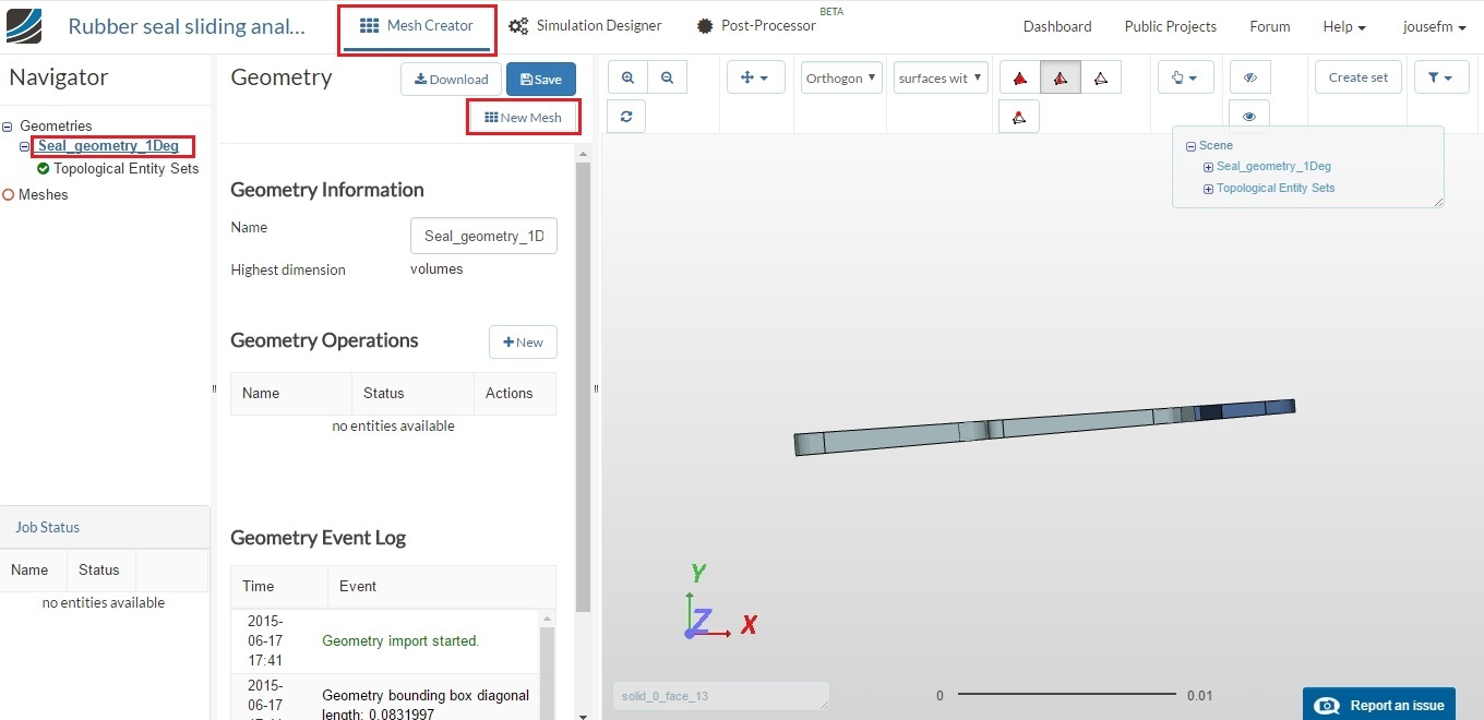
-
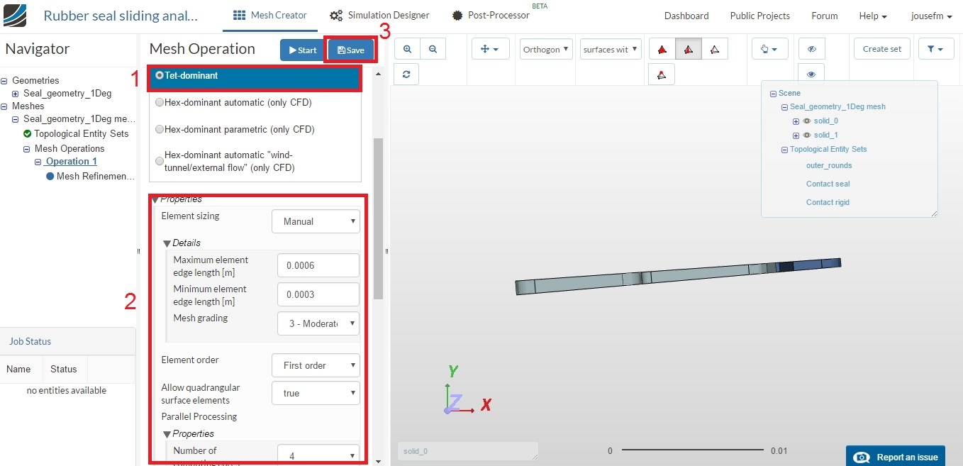
Select Tet-dominant [1] for the mesh and use the following parameters [2] - 0.0006 and 0.0003 as maximum and minimum mesh edge length respectively, First order for the desired mesh order, 3-Moderate fineness and 4 computing cores.
-
Save [3] the settings.
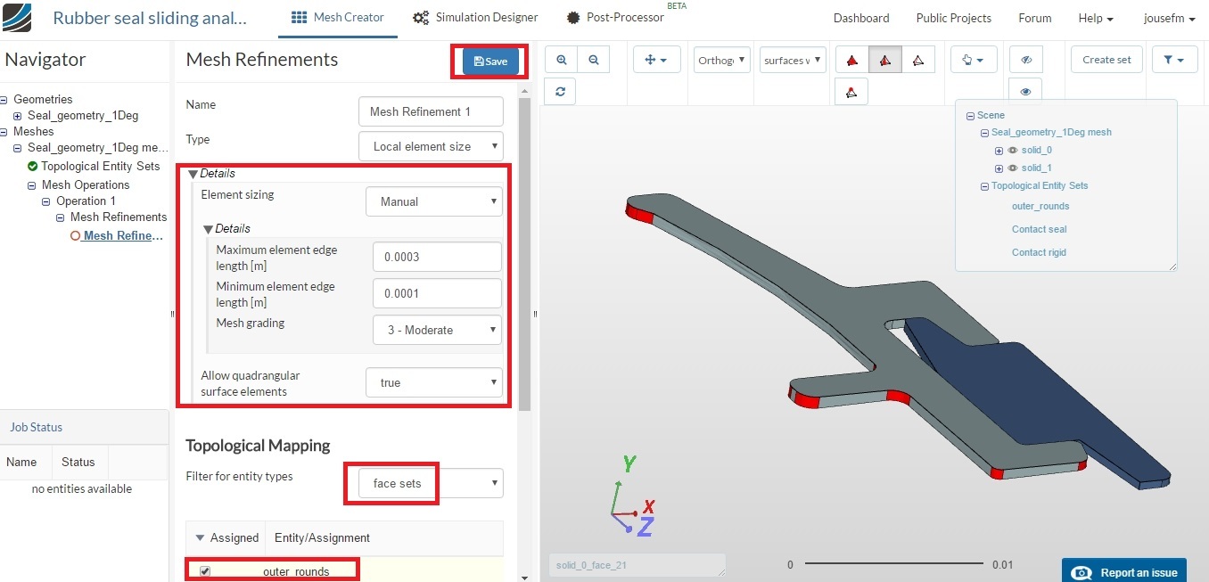
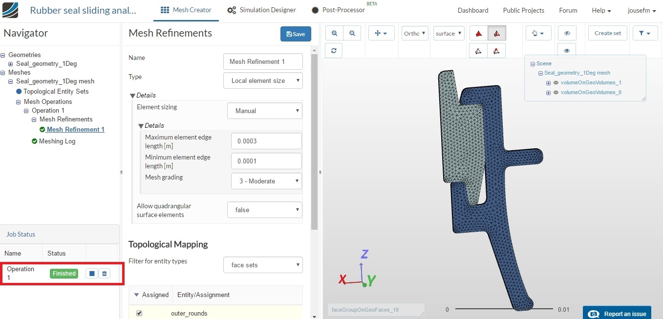
- To add a mesh refinement, click on New button in the bottom. This is done to locally refine small geometric features. In this geometry, some fillets are grouped into a topological set called outer_rounds, which needs to be refined.

- Use the parameters given in the figure below for local refinement at the fillets. Select face sets in the ‘Topolgical Mapping’, click on the outer_rounds and then Save the settings.
- Go back to Operation 1 and then click on Start button to start the meshing operation. The meshing job will start in a few moments and all computation is done via cloud computing.
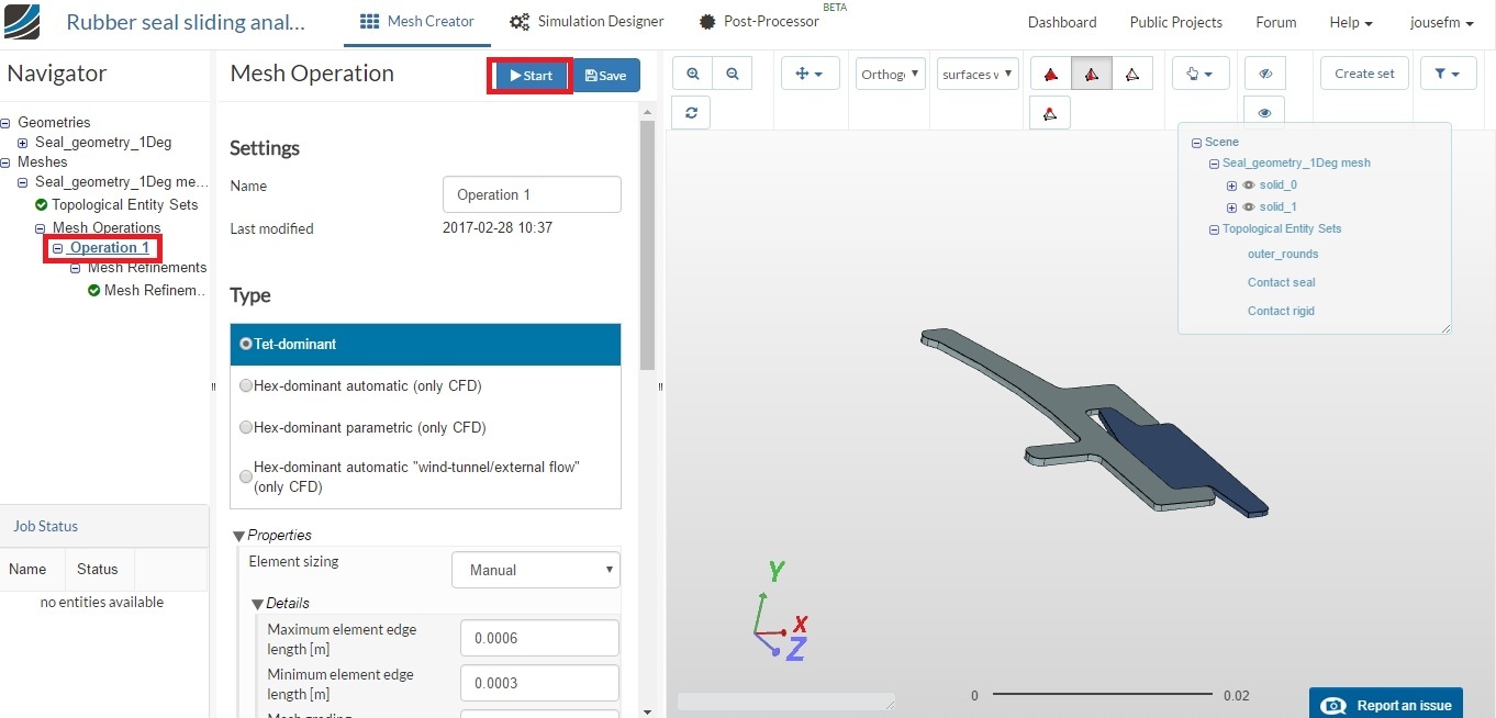
- The mesh operation takes about 1 min to complete and gives a Finished status in the lower left corner once it is over. The meshed geometry can be seen in the viewer.
Simulation Setup
-
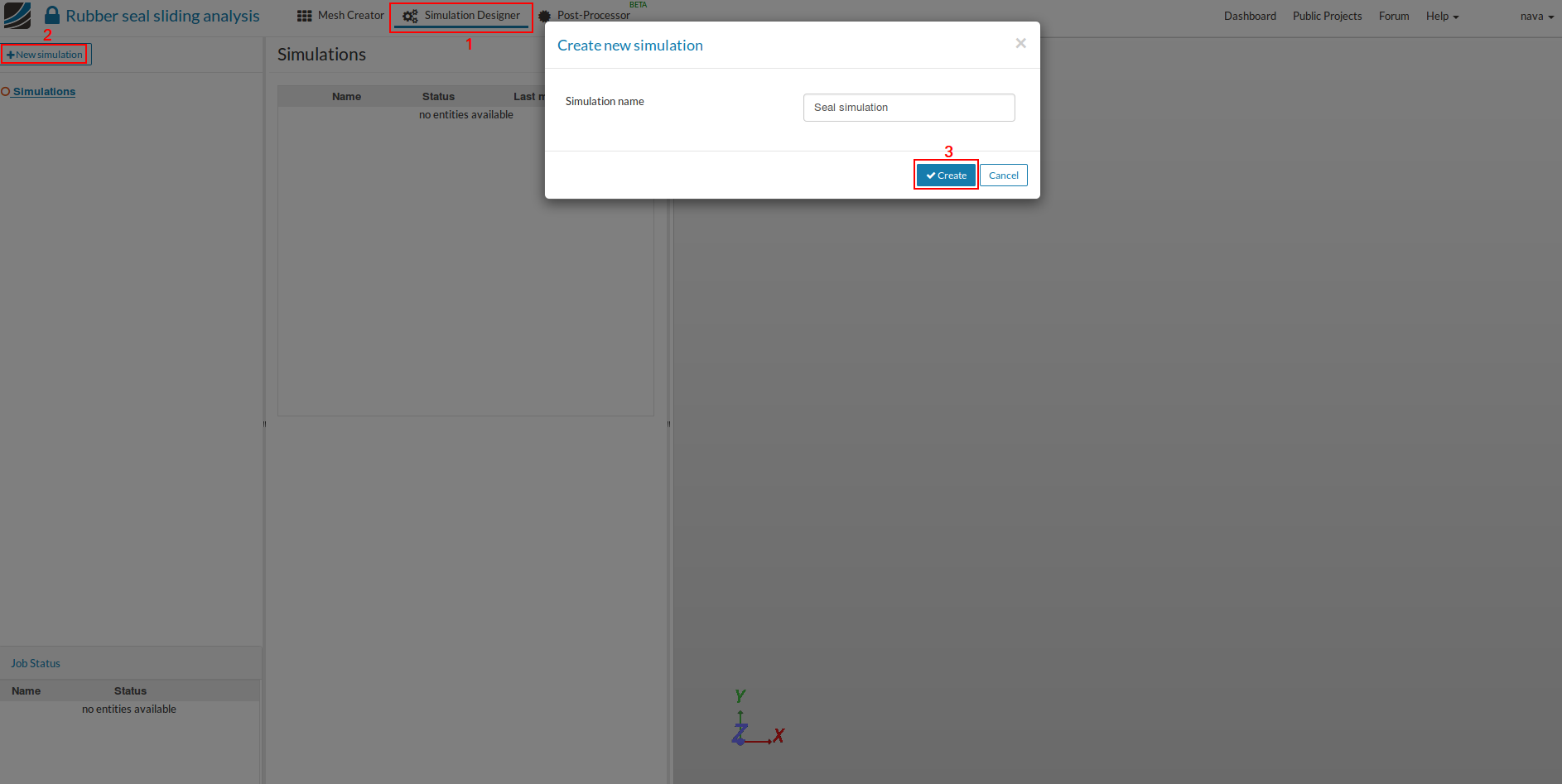
For setting up the simulation, switch to the Simulation Designer tab [1] and select New simulation [2].
-
A create new project window will pop-up. Give a suitable project name (optional) e.g. Seal simulation in this case and click Create [3].
- Since our simulation involves physical contact, select the analysis type Static analysis - advanced under Code_Aster (Solver Perspective), change Nonlinear analysis to true and click Save.
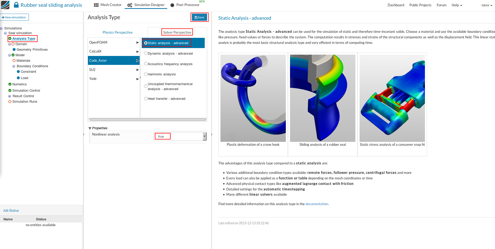
- After saving, the simulation tree now looks as shown below. Here the tree entries in red must be completed.

Domain selection
-
Click on Domain from the tree and select the mesh created from the previous task. Click on the Save button. The mesh will be automatically loaded in the viewer.
-
Furthermore, change render mode to Surfaces for a cleaner view.

Create Topological Entity Sets
- In this tutorial, we need 4 topology entity sets for specifying the boundary conditions and physical contacts.

- Click on the tree entry Topological Entity Sets.
Symmetry BC set:
- To create the first set, select the shown surface and click on the New from selection button to create a set named Symmetry BC set.

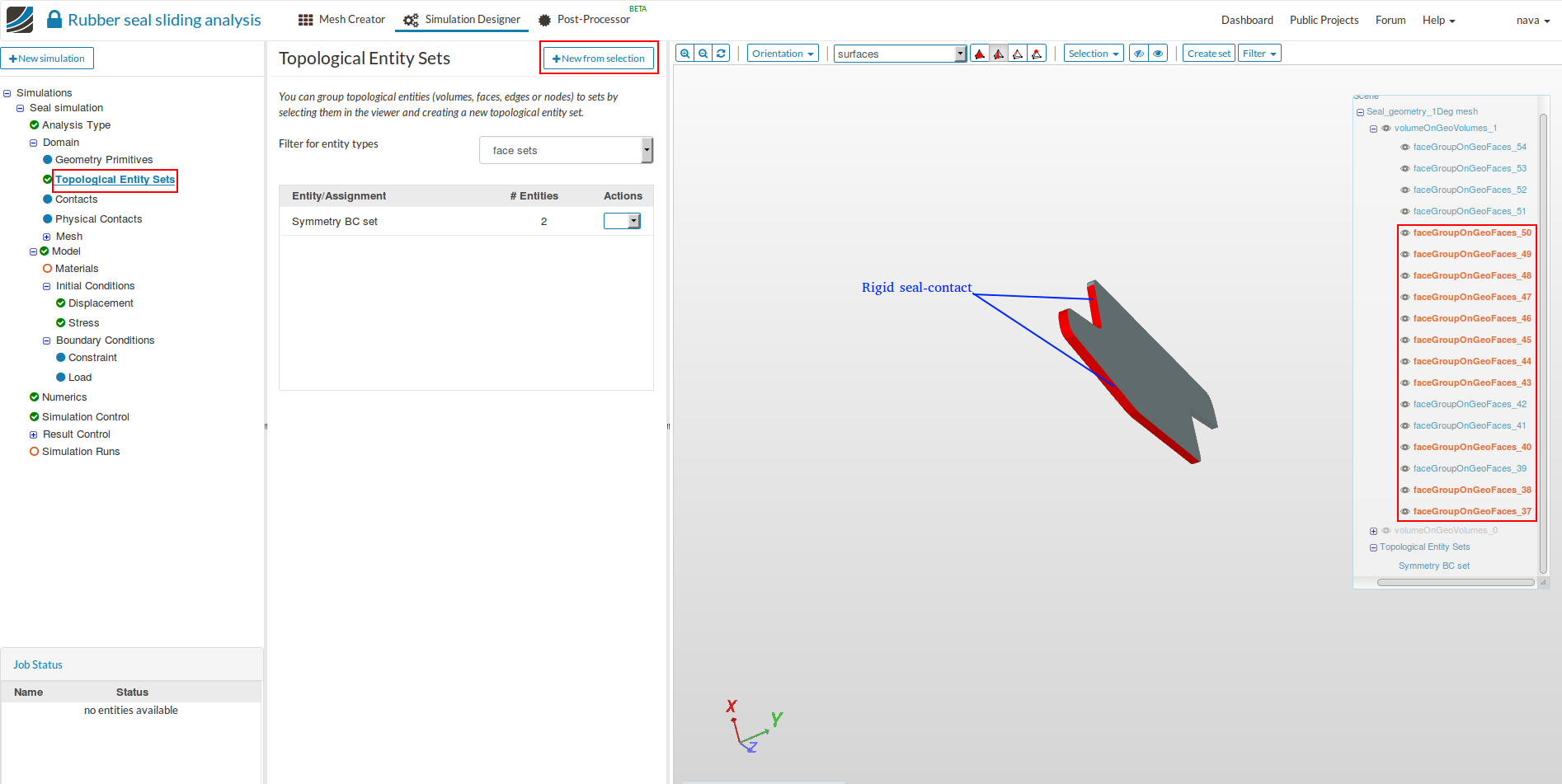
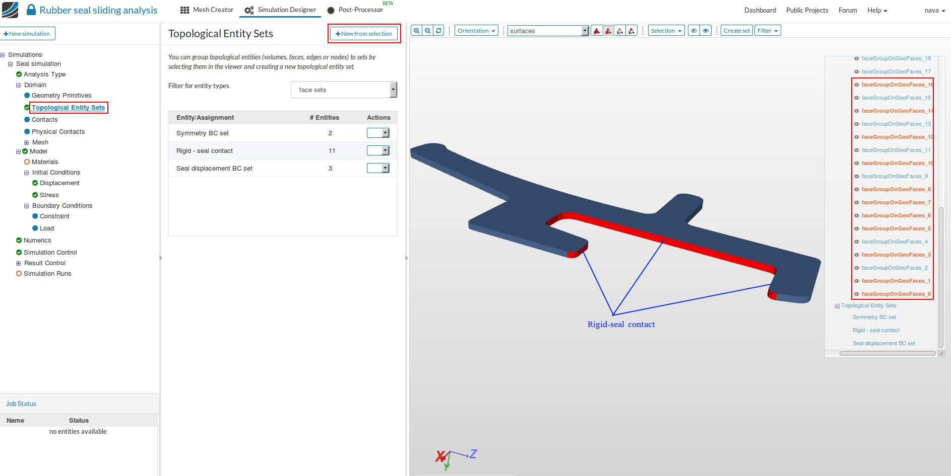
Rigid-seal contact:
- Follow the same step as above for creating the second topological set with a different set of faces as shown in the figure below. Here, we are making a set of faces from the rigid body which is in contact with the seal. For showing all the faces of this topological set, the seal body is hidden in the figure below.
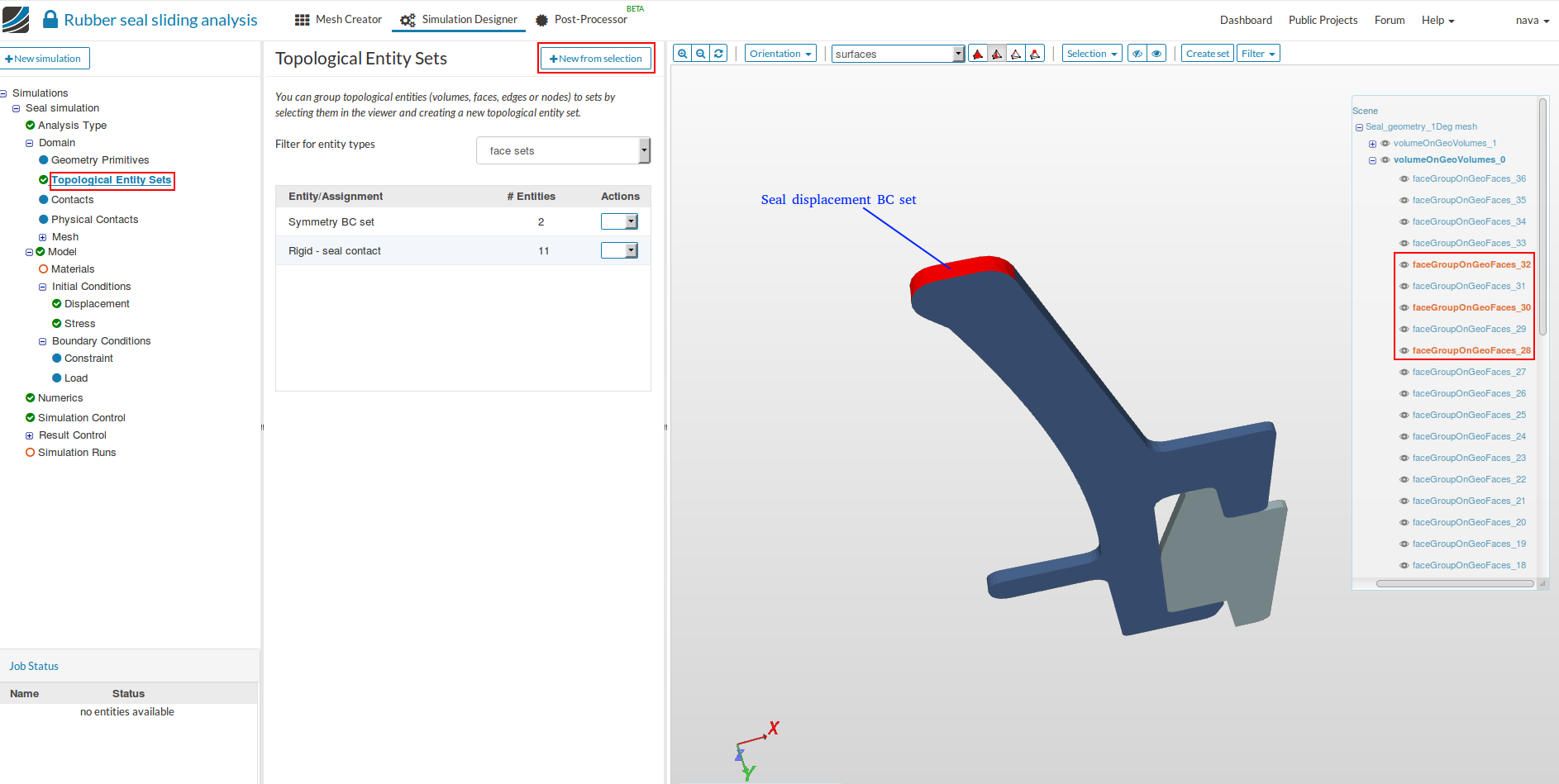
Seal displacement BC set:
- Follow the same step as above for creating the third topological set with a different set of faces as shown in the figure below. Here, we are making a set of faces from the seal body where displacement will be applied.
Seal-rigid contact:
- Follow the same step as above for creating the fourth topological set as shown in the figure below. Here, we are making a set of faces from the seal body which is in contact with the rigid body. For showing all the faces of this topological set, the rigid body is hidden in the figure below.
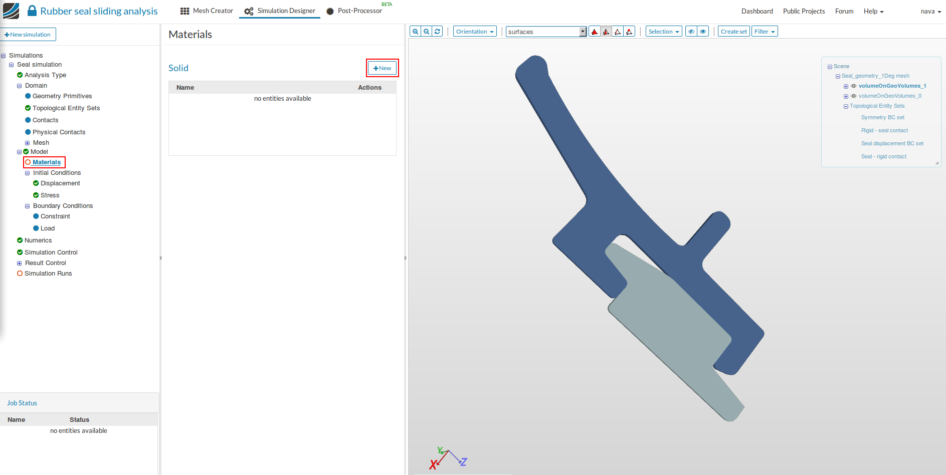
Select Solid Material
-
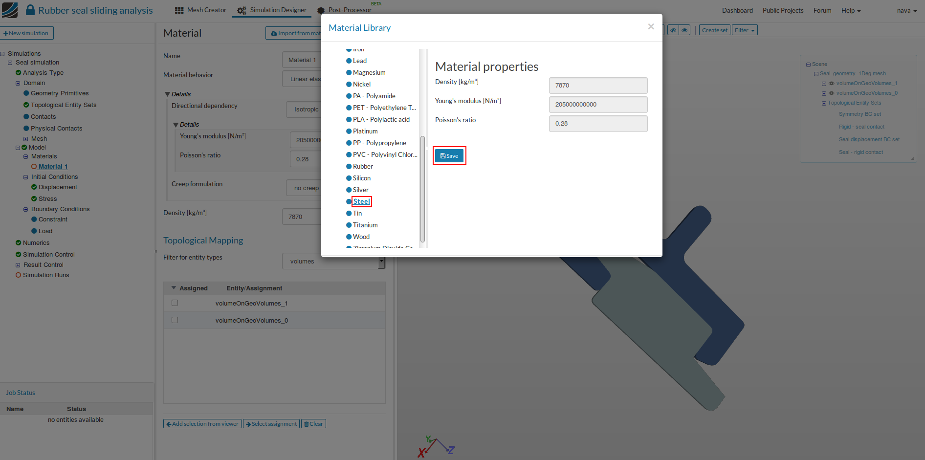
Now we will define material for our rigid body (Steel) and seal (Rubber). Select Material from the sub-tree and click New.
-
Click on Import from material library and select Steel and then Save.
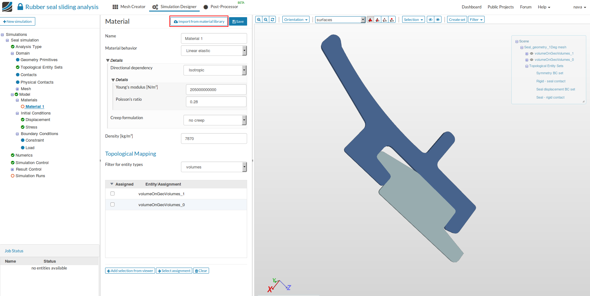
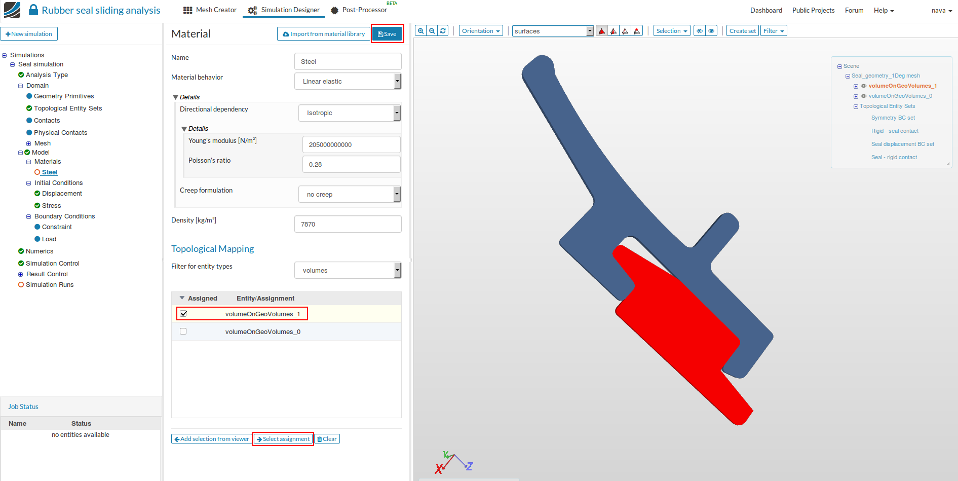
- Select volumeOnGeoVolumes1 (rigid body) to add the volume to which steel is assigned and then Save.
- You can highlight the selected volume by clicking on Select assignment.
- Similarly add rubber material for the seal following same steps as above.

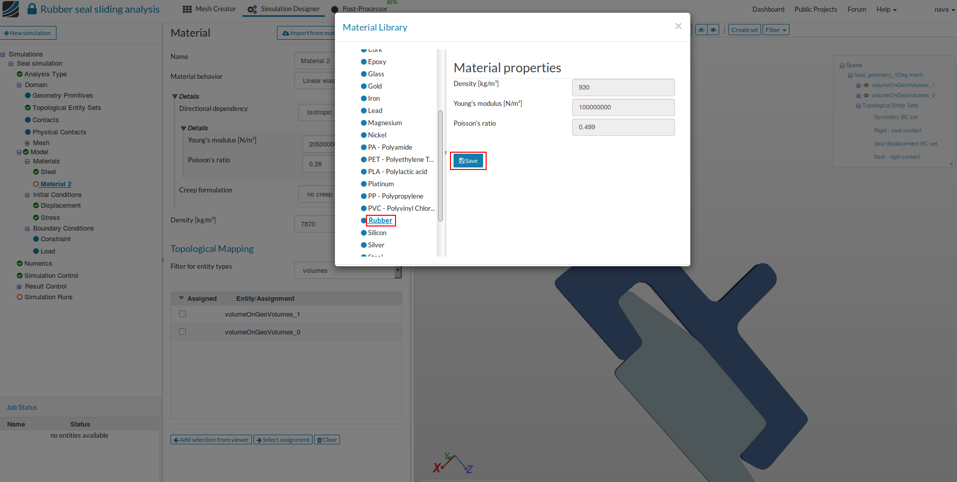
-
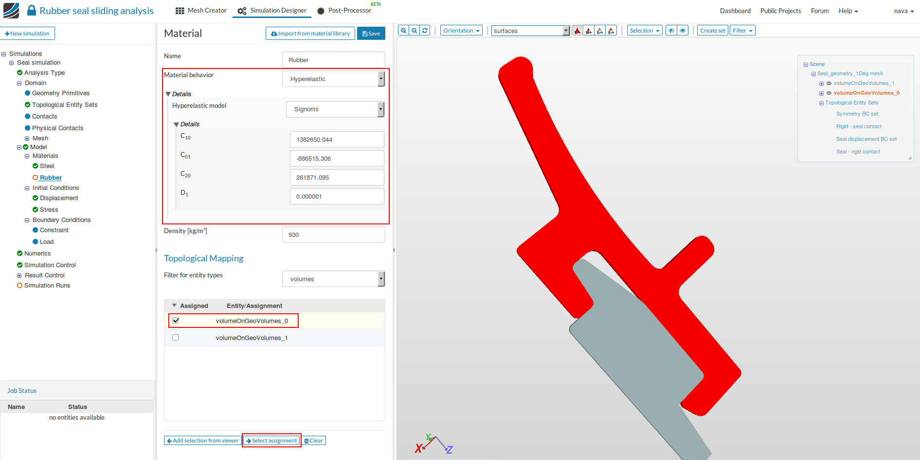
Select Hyperelastic for ‘Material behaviour’ and in the ‘Hyperelastic model’ choose Signorini. Use the parameters given in the figure below.
-
Select volumeOnGeoVolumes0 (seal) to add the volume to which rubber is assigned and then Save.
-
You can highlight the selected volume by clicking on Select assignment.
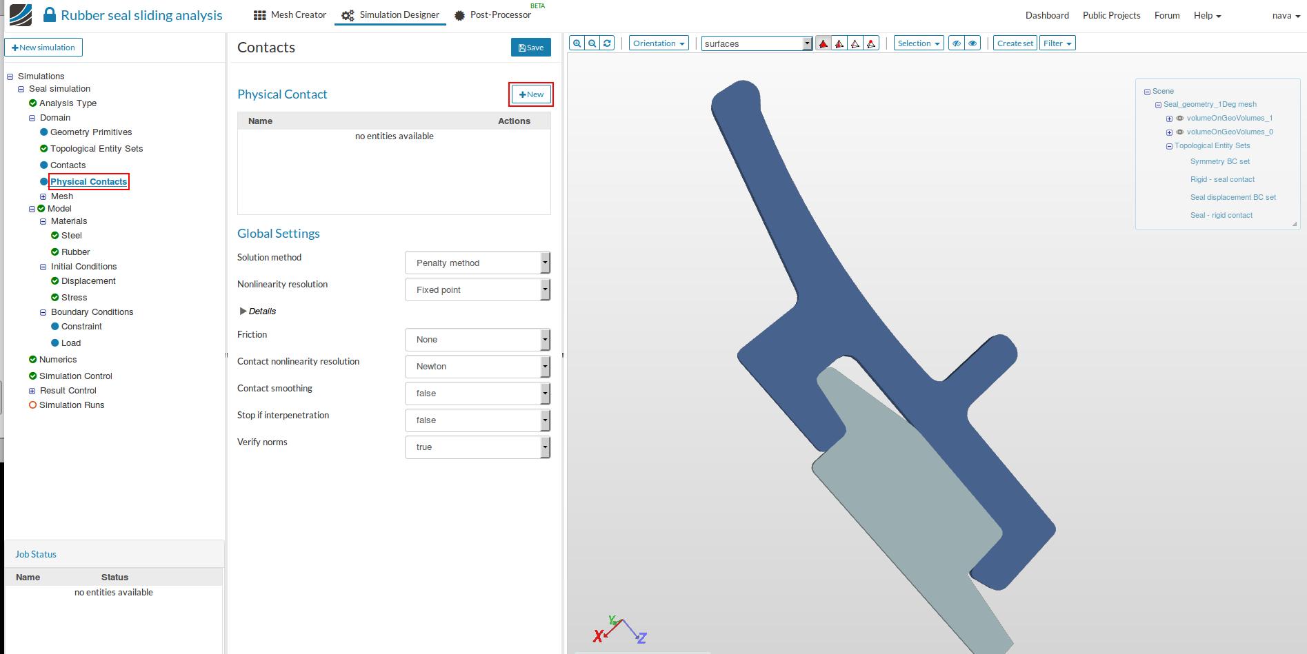
Physical Contacts
In this section we will define the physical contact between the seal and the rigid body. We are using penalty method for modelling the contact.
- Select Physical Contacts and then click on New. The Penalty method is available as default and don’t change any options here.
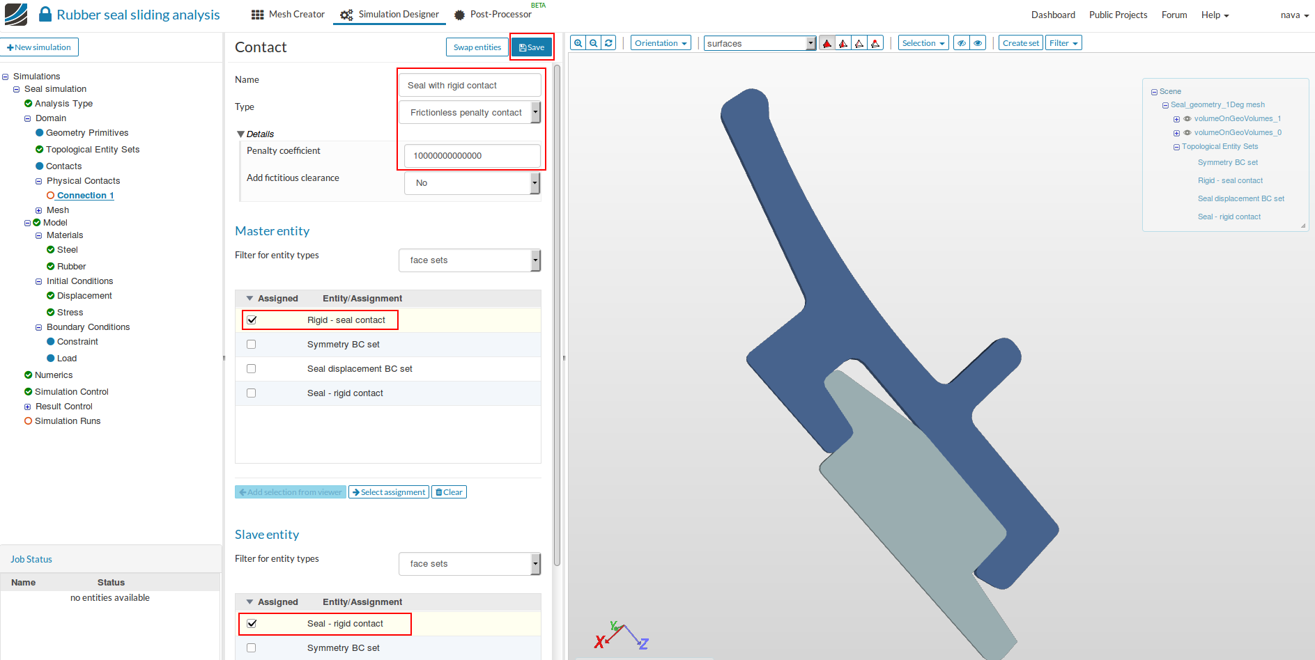
- Change the ‘Name’ to Seat with rigid contact (optional) and give a very high value of
‘Penalty factor’ ( 1e13). - Here, we are not considering friction at the contact, therefore choose Frictionless penalty contact as ‘Type’.
- Select Rigid-seat contact as a ‘Master entity’ and Seal-rigid contact as ‘Slave entity’ and then click Save.
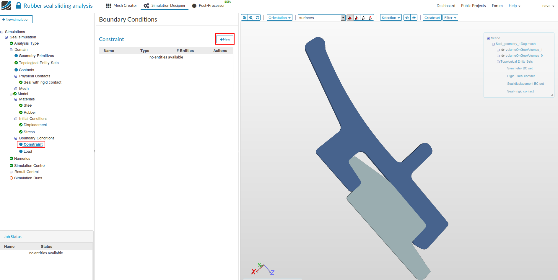
Boundary Conditions
In this section we will define the fixation of the rigid body, symmetry boundary conditions for seal along the circumferential direction for modelling axisymmetry and displacement of the seal body.
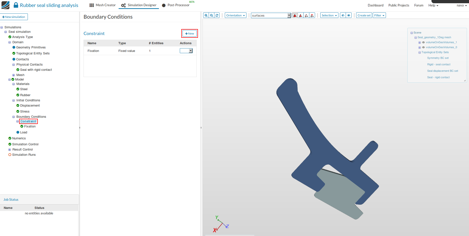
- Let’s first define fixation. Select Constraint in the tree and click New.
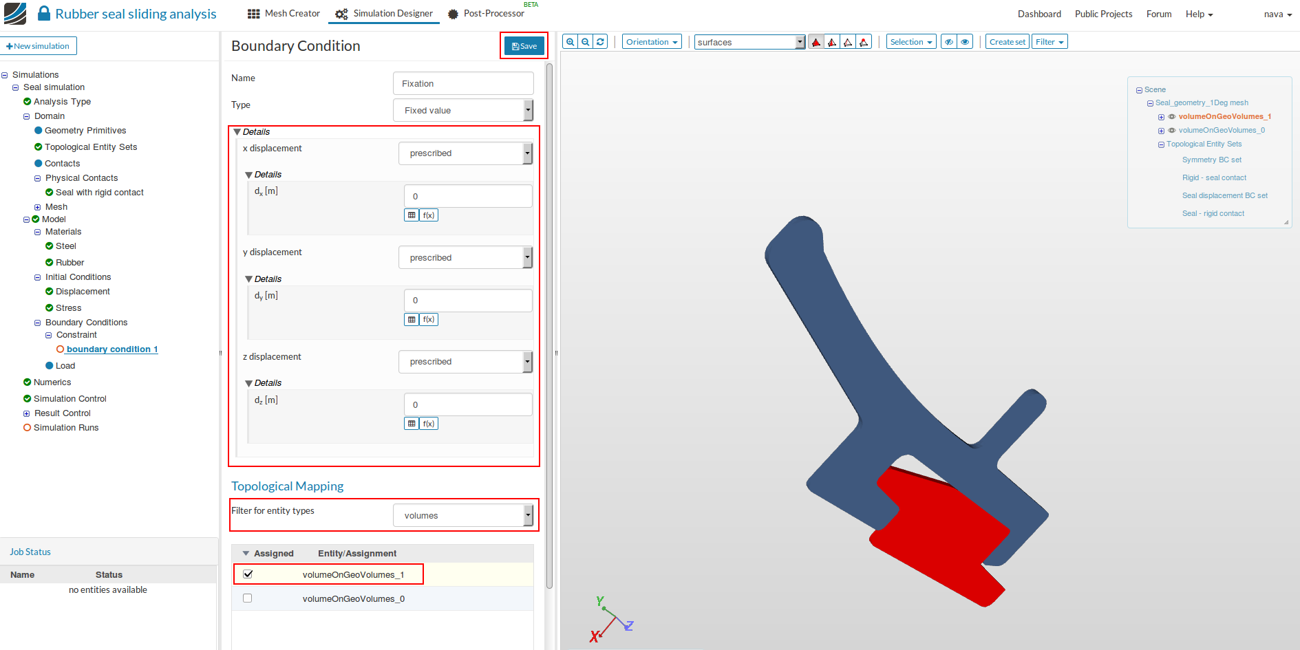
- Rename the Boundary condition to Fixation (optional). Choose the ‘Type’ Fixed value. Under Topological Mapping, change ‘Filter for entity types’ to volumes and select volumeOnGeoVolumes1 (rigid body). Then click Save.
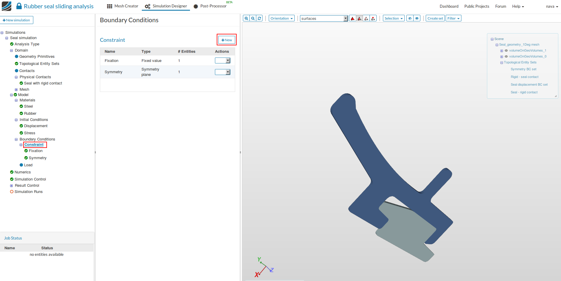
- For defining the symmetry boundary conditions, select Constraint in the tree and click New.
- Rename the Boundary condition to Symmetry (optional). Choose the ‘Type’ Symmetry plane. Under Topological Mapping, change ‘Filter for entity types’ to face sets and select Symmetry BC set. Then click ‘Save’.

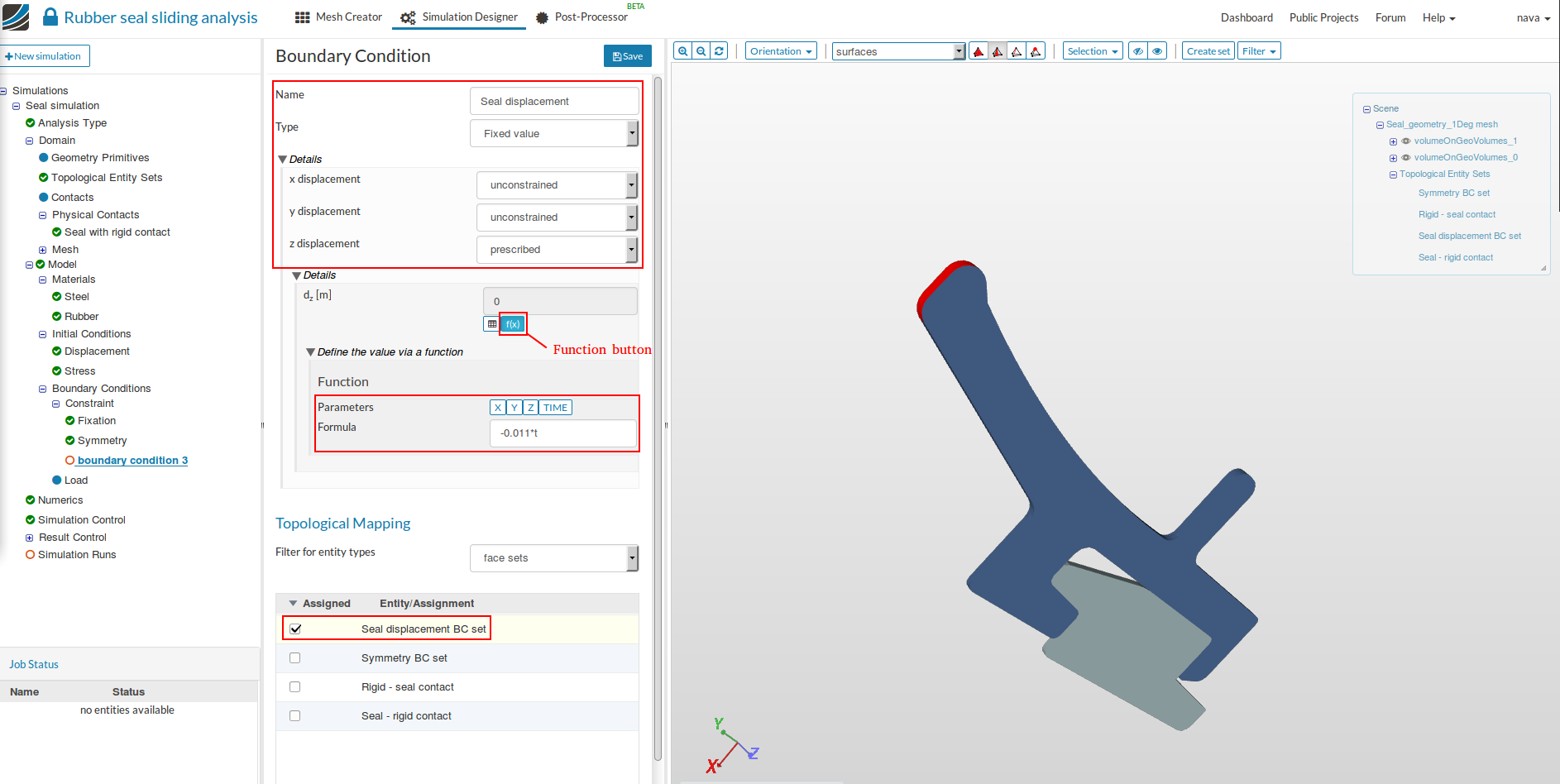
- For defining the seal displacement, select Constraint in the tree and click New.
- Rename the Boundary condition to Seal displacement (optional). Choose the ‘Type’ Fixed. Choose unconstrained for x and y displacement and for the z displacement, specify it as a function by clicking on ‘function button’ and give 0.011*t in the ‘Formula’.
- Under Topological Mapping, change ‘Filter for entity types’ to face sets and select Seal displacement BC set. Then click Save.
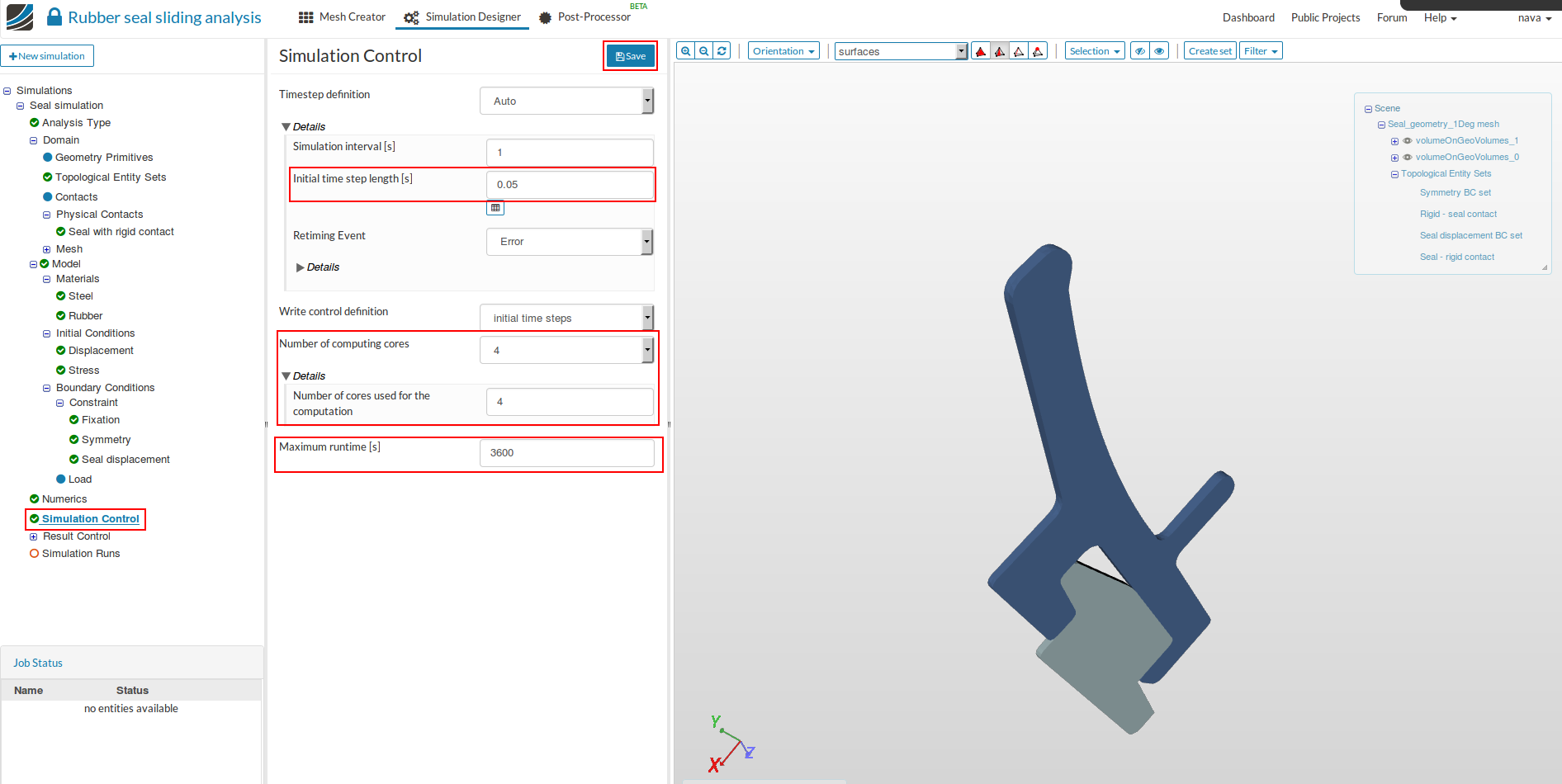
Simulation Control
- Click on Simulation control and change ‘Initial time step length [s]’ to 0.05 under details of ‘Timestep definition’, ‘Number of computing cores’ to 4, under details ‘Number of cores used for the computation’ to 4 and Maximum runtime [s] to 3600.
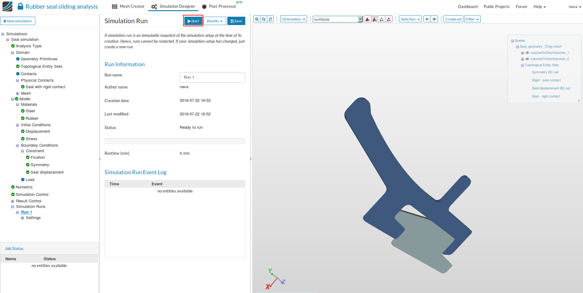
- Click on Simulation runs and create a new run.


- The new run will be created under Simulation Runs. Click Start to run the simulation.
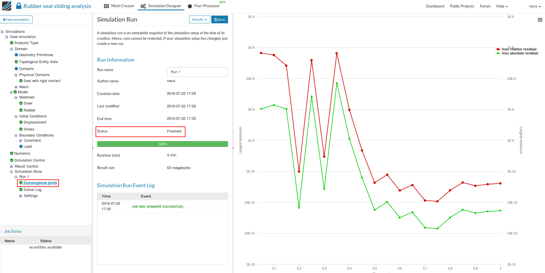
- The run takes approximately 4min. After the run is finished you can see the ‘Status’ as Finshed and the convergence plot can be seen by selecting Convergence plots.
Post-processing
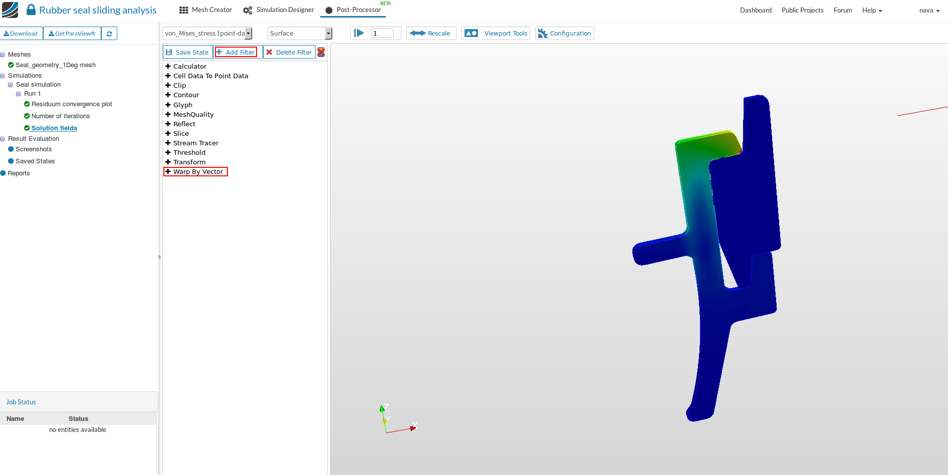
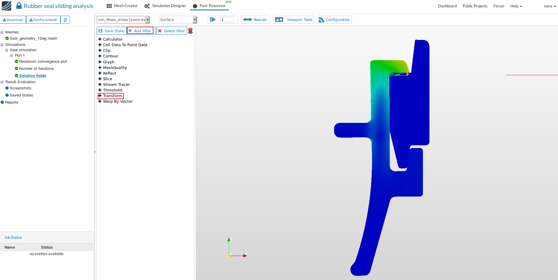
- Once the simulation is over, click on Post-processor tab to view the results and select Solution fields.

- In order to see the deformed shape of the rubber seal, click on Add Filter and then Warp by Vector.
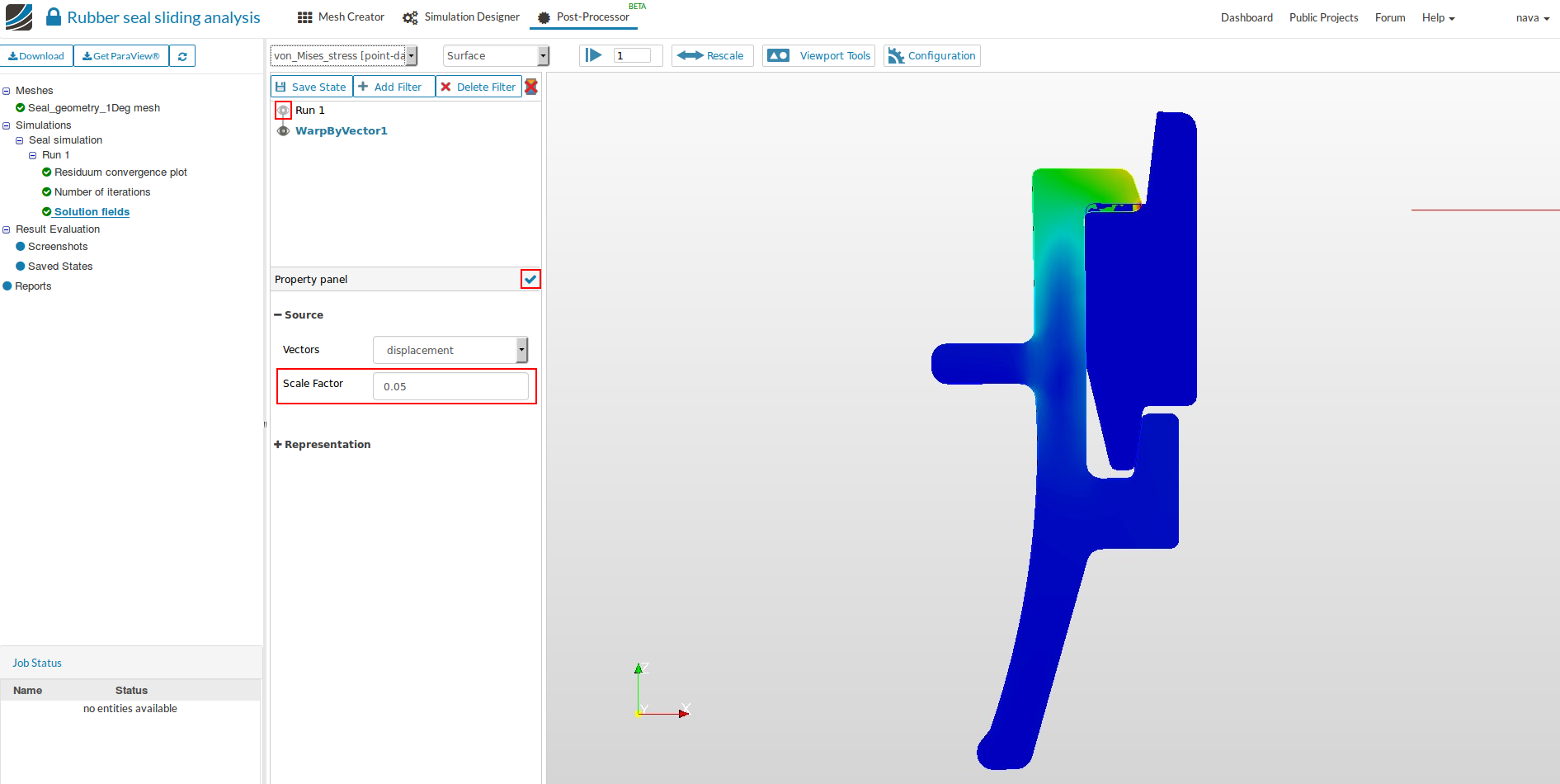
- Give a suitable ‘Scale Factor’ for scaling the deformation (say 0.005). Click on tick mark to apply the changes. You will see both deformed and undeformed geometry. In order to hide the undeformed geometry, click on the ‘Eye button’ at the left of Run 1.
-
The result you see in the viewer window is only a 1 deg sector of the whole circular symmetric body. Since the problem is circular symmetric, the stress and deformation result will be also symmetric.
-
Hence, the result of the complete body can obtained by revolving the result along the axis. This can be done by clicking on Add Filter and then Transform.
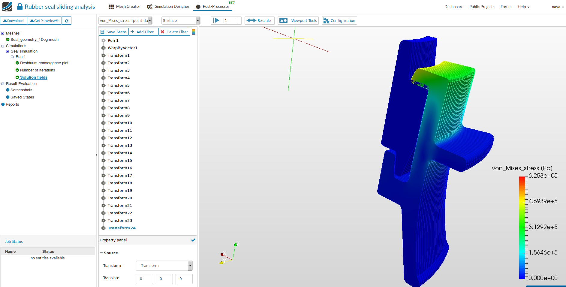
- Since the axis of symmetry is z axis and the sector is of 1 deg, give the value 1 for the ‘Rotate’ under 3rd column. Click on the tick mark to reflect the changes. This operation will create a copy of the result moved by 1 deg.

- Repeat the same step 24 times to visualise the result for a 25 deg sector. The figure below shows von Mises stress of the seal.
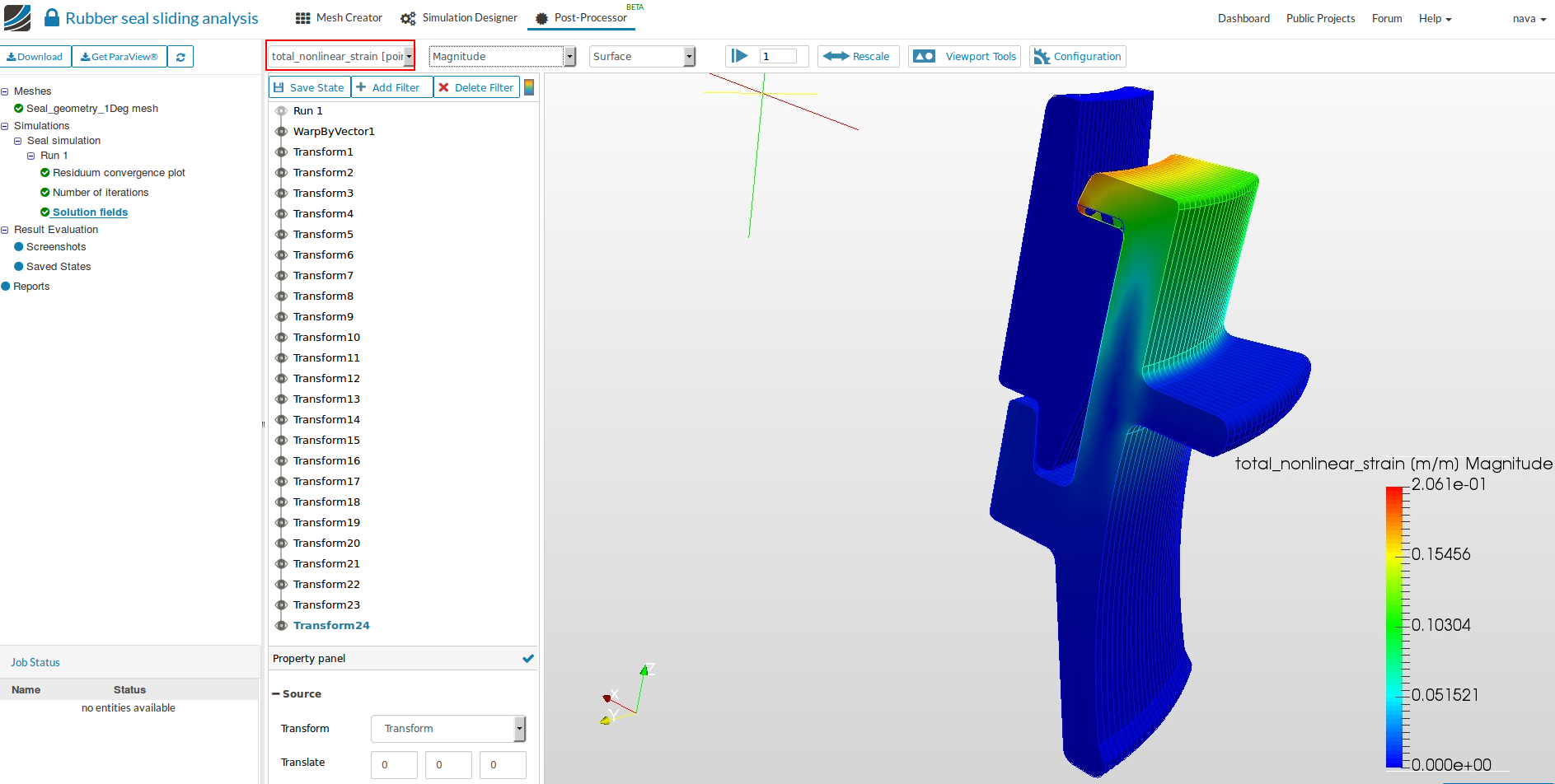
- You can also view total non linear strain of the body by selecting total_non_linear_strain for all the filters.
- This can be done more elegantly in Paraview. Following link provides details on postprocessing in Paraview.
