NOTE: This tutorial was updated on 10/2016 to match the updated version of the platform
If you would like to watch the fourth session of the Drone Workshop again or in the case you missed it, you can access the full recording below.
 - Frequency Analysis of a Structural Frame")
Background:
Much effort is going into the investigation of vibrations when developing an aerial vehicle. Of further interest here are two main aspects: What are the design-dependent natural frequencies of the vehicle (eigenfrequencies) and how does the drone reacts to external periodic excitations at this specific frequencies.
This information are important to improve the dynamic stiffness of the drone while operating and to avoid long-term harm to the material like fatigue fractures.
Exercise:
To perform such a vibration analysis it is therefore necessary two run two different simulations. According to the preliminaries of the preface we will first run a Frequency Analysis to identify the eigenfrequencies of the drone design. This results will be used in Level 2 for the correct simulation setup.
Step-by-Step-Instructions:
Meshing:
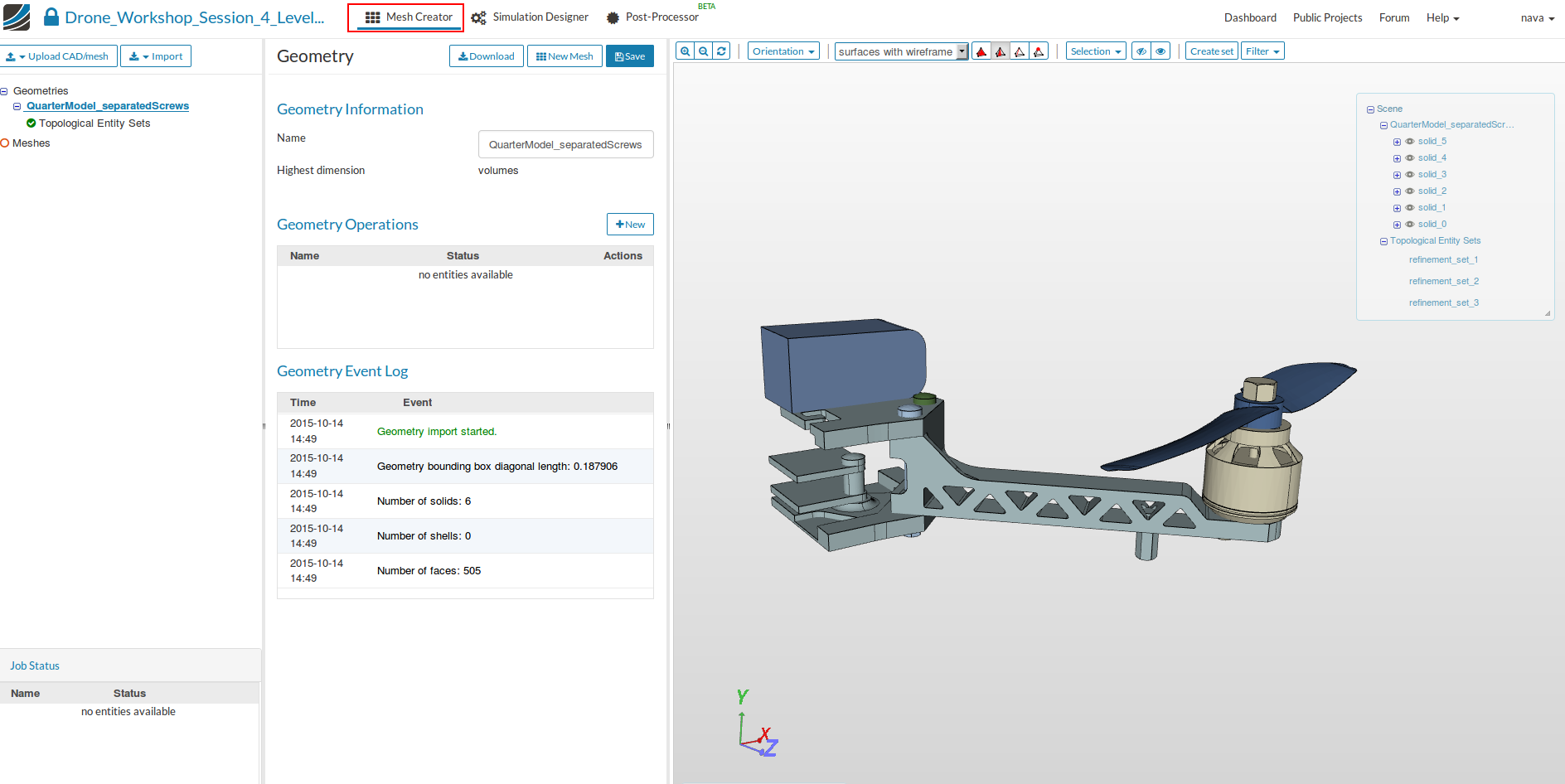
First of all you have to import the geometries into your SimScale workspace. For this, you only have to click on this link and a project with everything you need will be added to your workspace. ease note that this can take several minutes. By default you will be in the Mesh Creator tab.
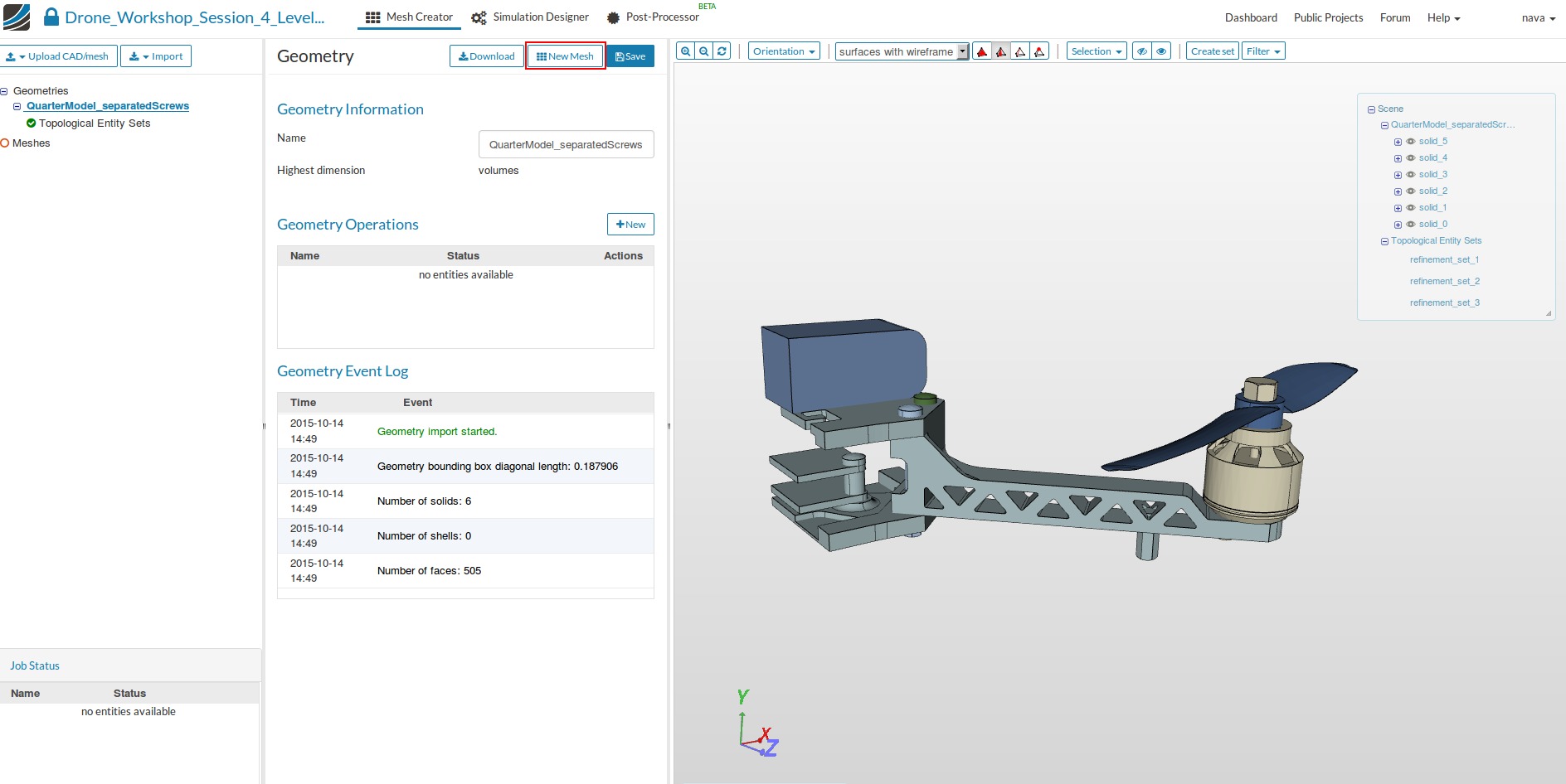
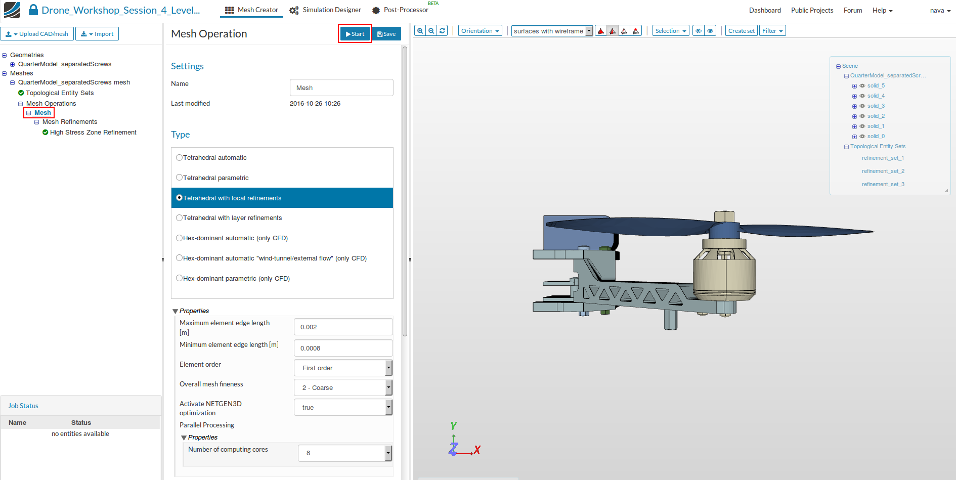
- Click on the New Mesh item in the project tree. This will open an additional column in the middle.
- Select Tetrahedral with local refinement from the list and define following parameters:
- Name: Mesh
- Maximum mesh edge length: 0.002
- Minimal mesh edge length: 0.0008
- Overall mesh fineness: 2 - Coarse
- Activate NETGEN3D: True
- Number of processors: 8
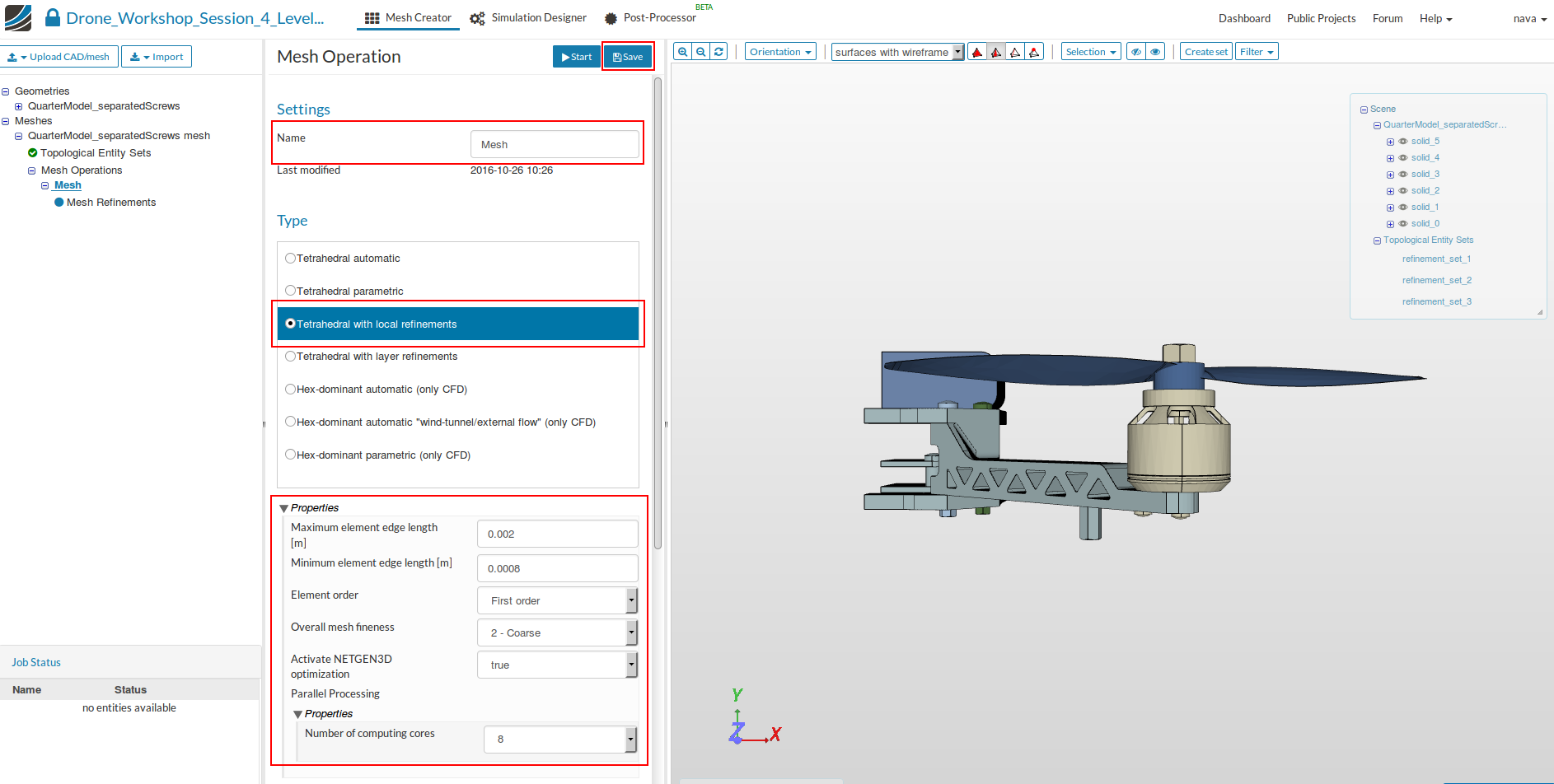
- Save the settings by clicking on Save button.
Now we have defined a range for the base mesh size which is fine for regions where we are not expecting high stress. Here you should keep in mind that, in general, the mesh size is related to the local accuracy of the simulation. It is therefore necessary to refine the mesh in those areas where high stresses are expected.
We will now apply local refinements on faces where we expect high stresses.
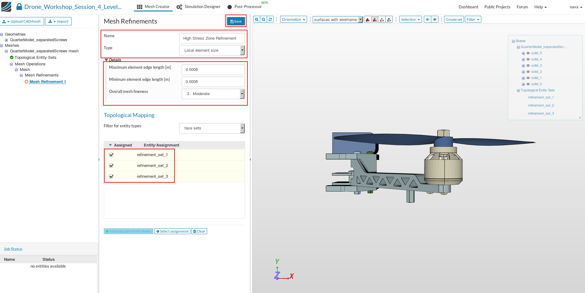
- Click on the New button near the Mesh Refinements option which will add a new sub-item to the project tree. Now you can specify the mesh refinement.
- Name: High Stress Zone Refinement
- Maximum mesh edge length: 0.0008
- Minimal mesh edge length: 0.0008
- Overall mesh fineness: 3 - Moderate
- Next, select the faces you want to apply this refinement by using the list below. Since the face selection would take lot of time for this mesh, we have prepared a ready-to-use face set. To use this sets, please change the Filter for entity type to face sets and select refinement_set_1, refinement_set_2 and refinement_set_3.
- Finally Save the settings.
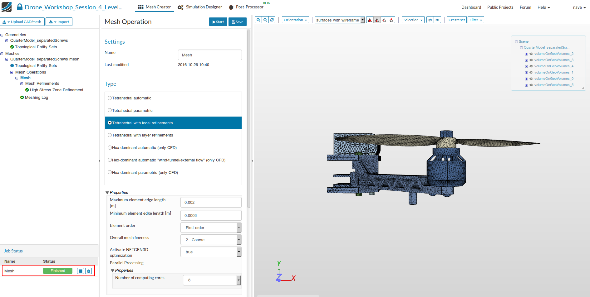
- Now our mesh is ready for computation. Click on the Mesh in the project tree and click the Start button. The meshing job will start in a few moments and all computation is done via cloud computing.
Once the mesh computation is completed, finished status will appear in the lower left corner.
Simulation Setup
-
After the mesh is completed we will set up the simulation. Click on the Simulation Designer button in the main ribbon bar.
-
Click on the New button to create a simulation.
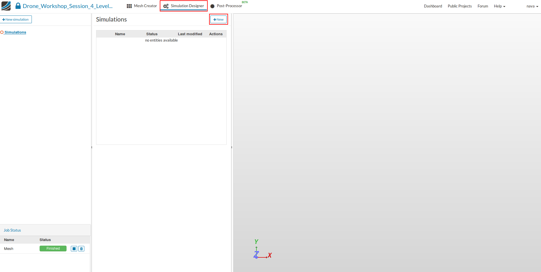
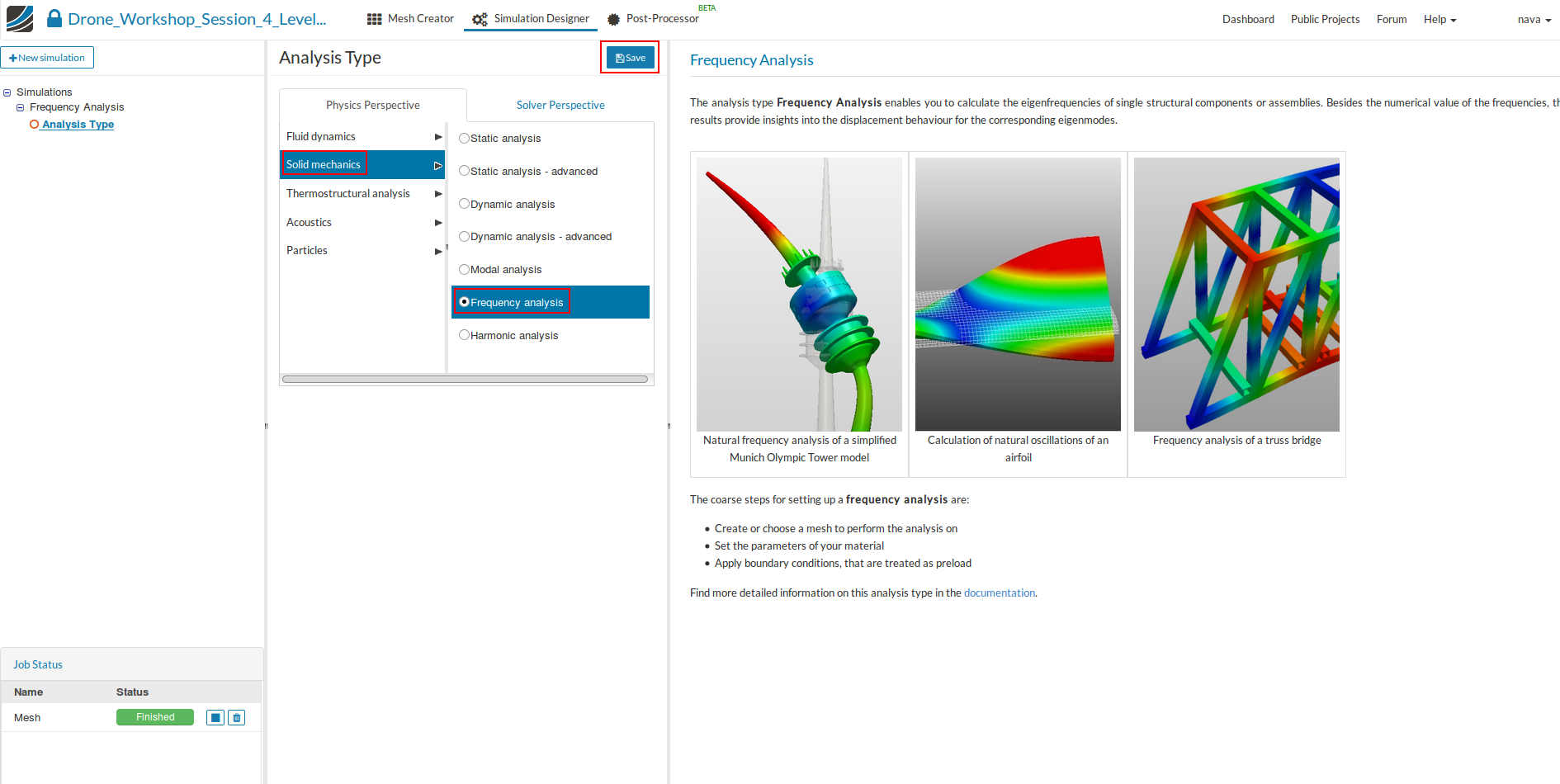
This will open an additional column in the middle. Here you can select the type of simulation you want to run. In our case we will run a Frequency Analysis simulation.
- Select Frequency Analysis option and then Save the settings.
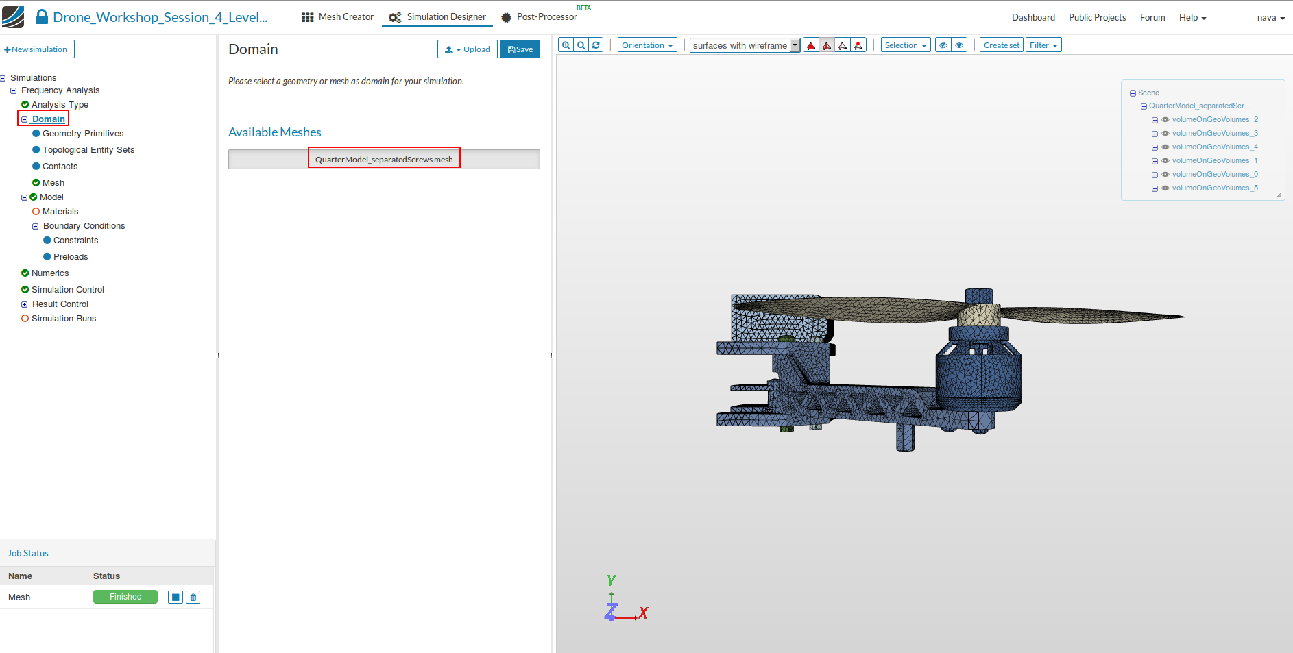
Domain
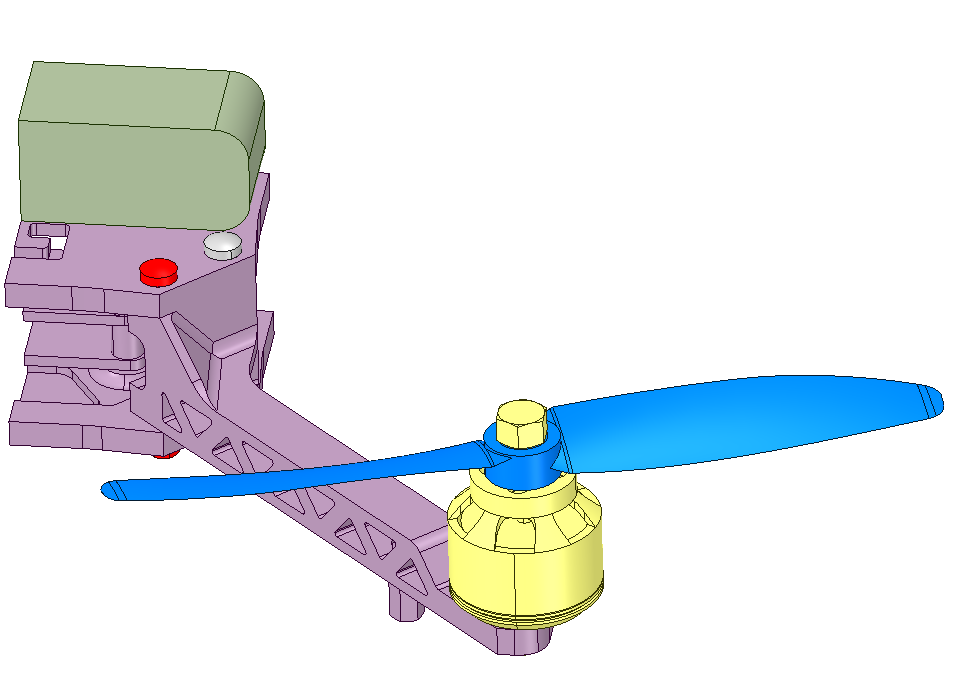
Next you have to specify which mesh you want to use for your simulation. Click on the Domain item in the project tree and select QuarterModel_separatedScrews mesh from the menu which disappears in the middle column. Don’t forget to Save your selection.
Topological Entity Sets
Before proceeding with the simulation setup we will create Topological Entity Sets which we will use for the next steps. They allow to group multiple entities from the same type.
We will create four different face sets by selecting the faces we want to group graphically.
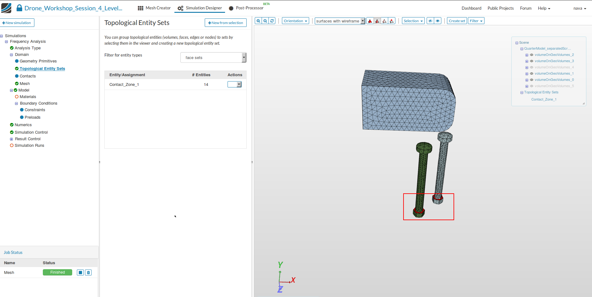
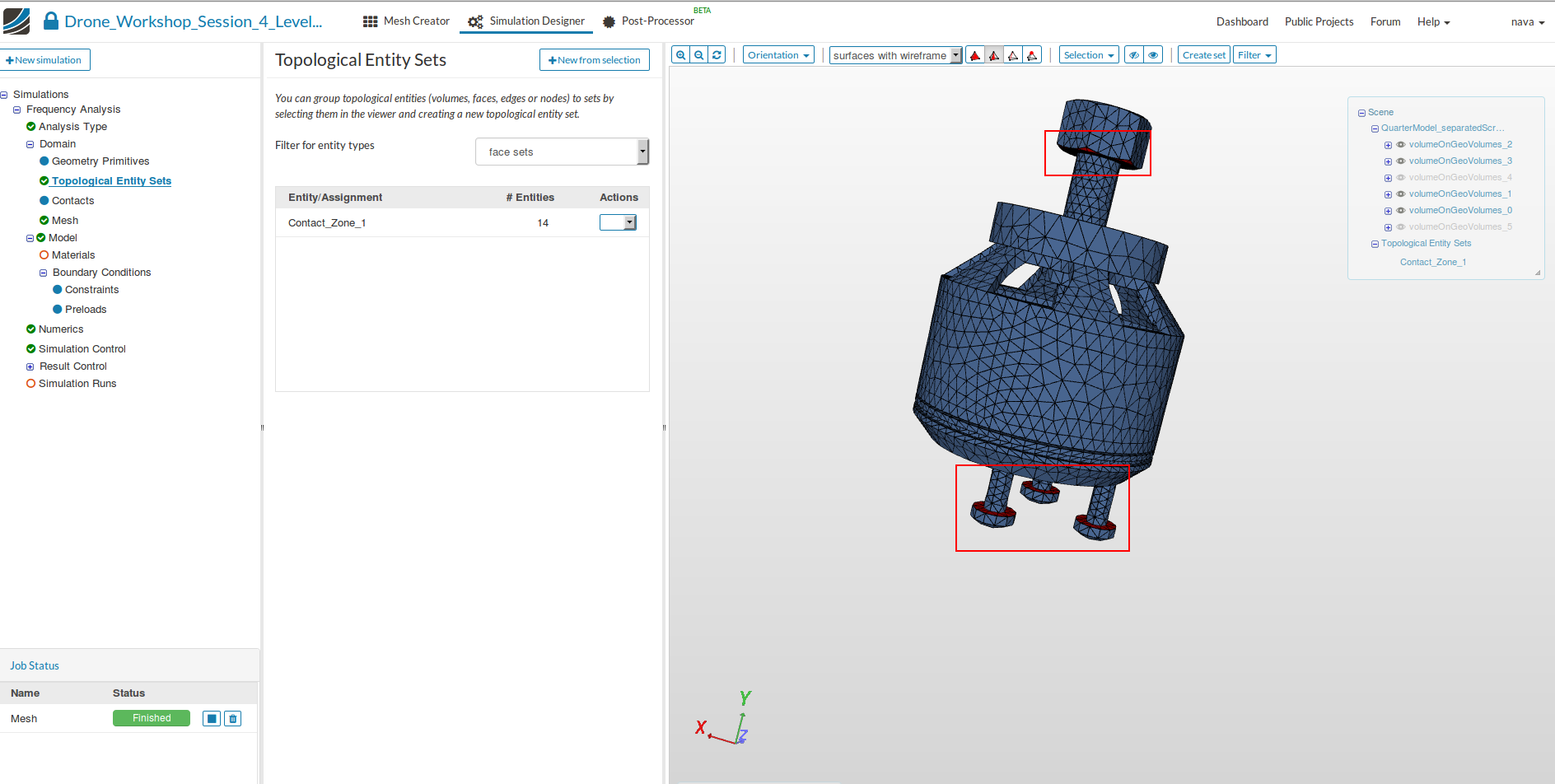
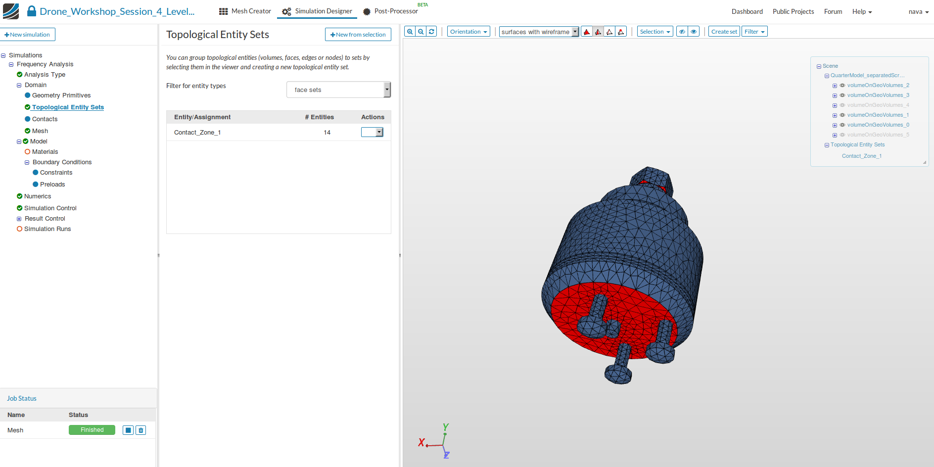
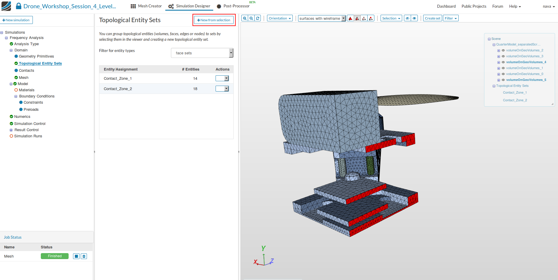
Contact_Zone_1 (14 faces)
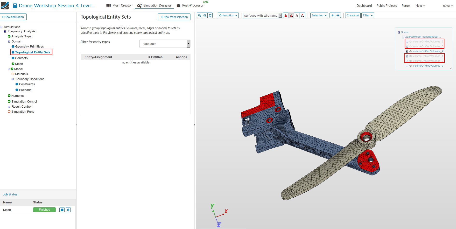
This face set should contain all Master entities for the contact definition. To be able to select the surfaces it is necessary to hide some of the volumes of the mesh.
-
Hide therefore the following volumes by clicking the eye symbol: volumeOnGeoVolumes_0, volumeOnGeoVolumes_1, volumeOnGeoVolumes_2, volumeOnGeoVolumes_3.
-
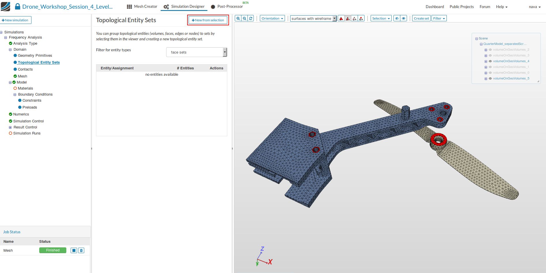
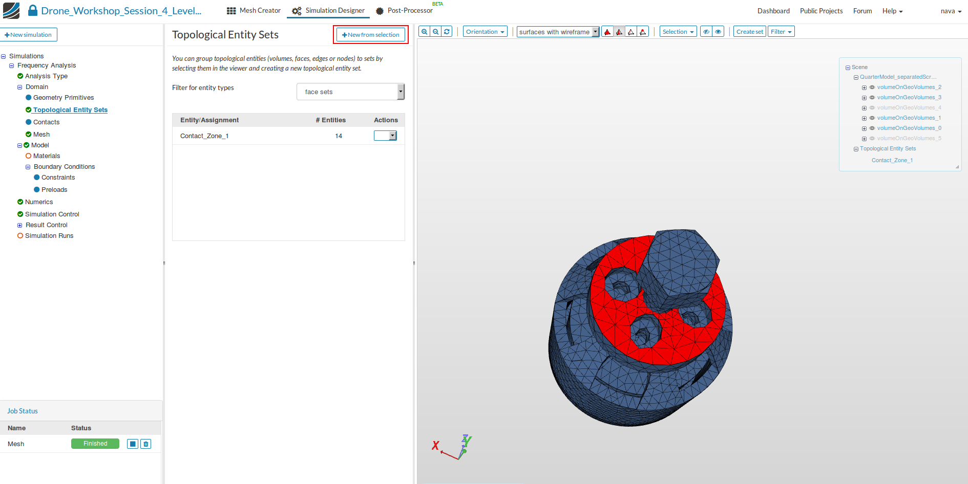
Go to Topological Entity Sets in the project tree and then select all the 14 faces which are needed. Please use the images below to identify the faces you need.
-
Click on New from selection and give it a suitable name - Contact_Zone_1 (optional).
Contact_Zone_2 (18 faces)
This face set should contain all Slave entities for the contact definition. To be able to select the surfaces it is necessary to hide some of the volumes of the mesh.
- Hide therefore the following volumes by clicking the eye symbol: volumeOnGeoVolumes_4, volumeOnGeoVolumes_5
Now you are able to select the 18 faces which are needed. Please use the images below to identify the faces you need.
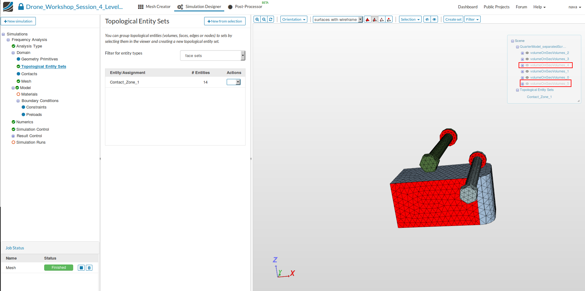
- Click on New from selection and then give this set a suitable name - Contact_Zone_2 (optional).
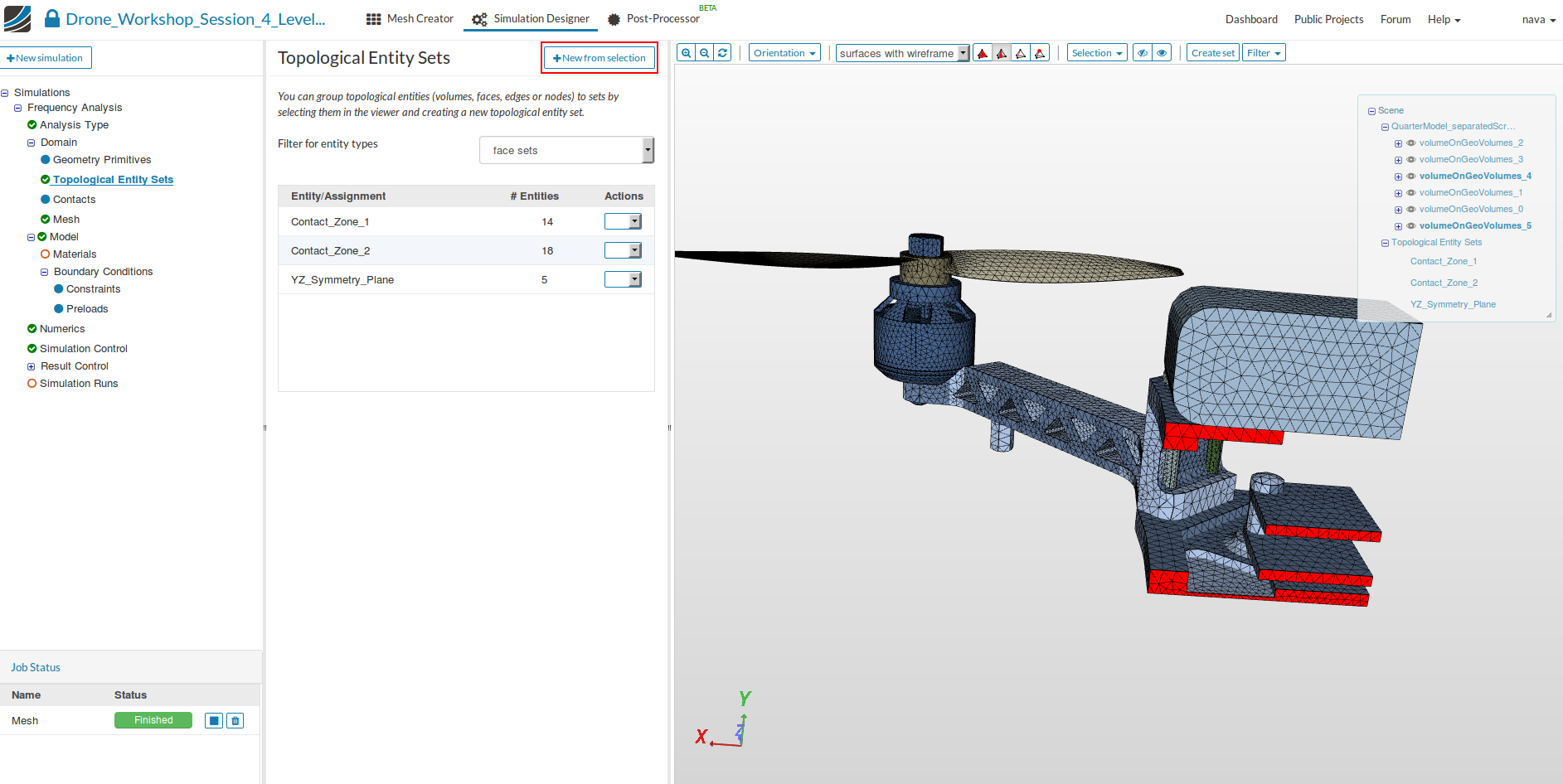
In the following we will define two Topological Entity Sets for the two symmetry planes. Please note that for frequency and harmonic analysis it is necessary to not ‘overcontraint’ the simulation. You should therefore NOT include the faces of the battery to this face set.
YZ_Symmetry_Plane (5 faces)
This face set should contain all faces of the drone chassis (volumeOnGeoVolumes_5) which are in the YZ symmetry plane.
-
Select the faces according to the image below and create the entity set following the same steps as above.
-
Specify the name to be YZ_Symmetry_Plane.
XY_Symmetry_Plane (4 faces)
This face set should contain all faces of the drone chassis (volumeOnGeoVolumes_5) which are in the XY symmetry plane.
-
Select the faces according to the image below and create the entity set following the same steps as above.
-
Specify the name to be XY_Symmetry_Plane.
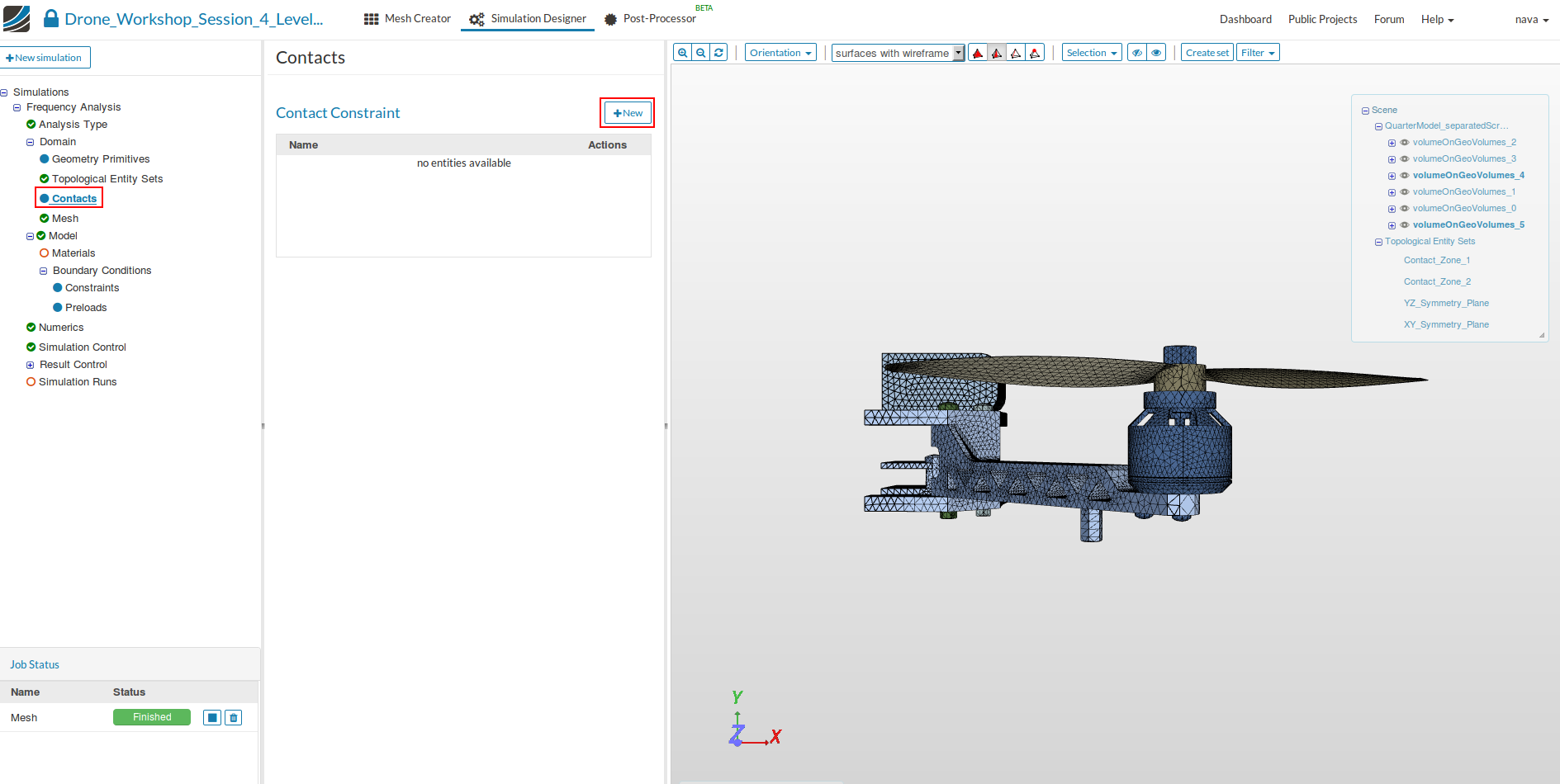
You can see all the created topological sets in the figure below.

Contacts
Since we are simulating an assembly of two parts, it is necessary to define Contacts which are describing the kinematic behaviour of the parts.
- Click on the Contacts item in the project tree which will open a new middle column menu where you can add new contacts by clicking on the New button.
In contrast to the last two homeworks, today we will define all kinematic dependencies in one contact.
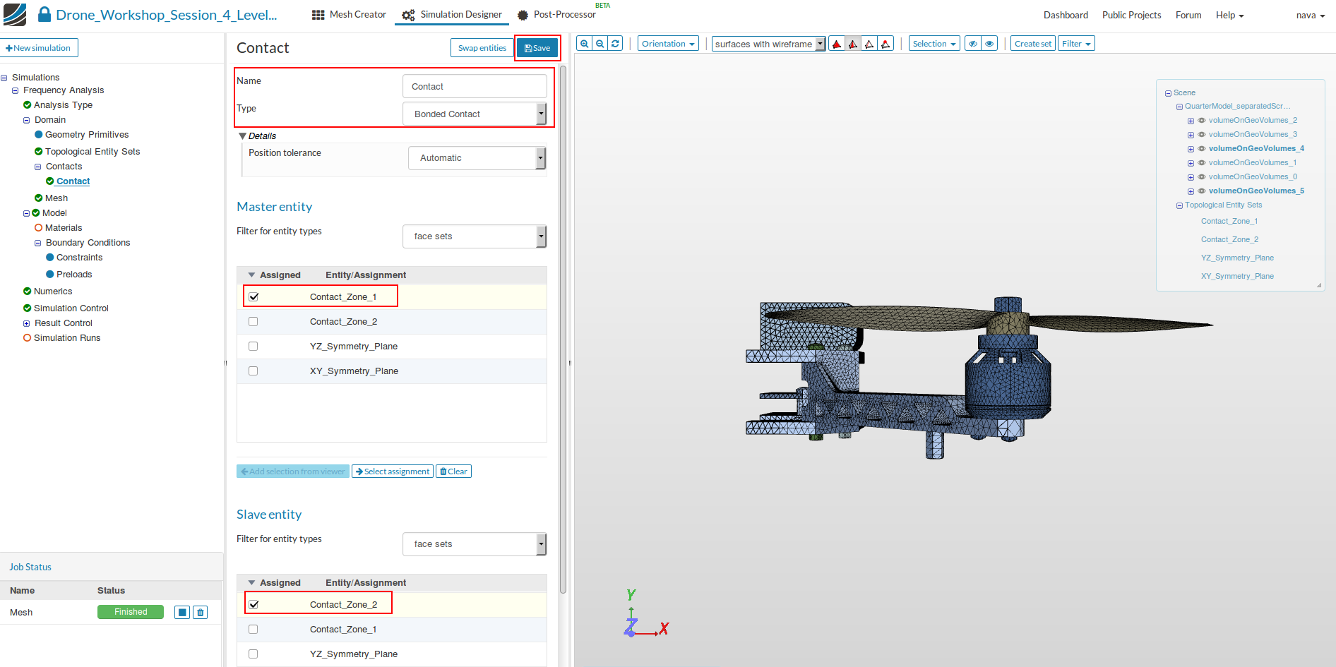
Contact
In this contact we will fix the assembly made of the battery, the frame, the screws, the engine and the propeller. Instead of selecting the faces for master and slave entity from the list or graphically we will use the face sets we created some minutes ago.
- Specify the following parameters:
- Name: Contact
- Type: Bonded Contact
- Master entity: Contact_Zone_1
- Slave entity: Contact_Zone_2
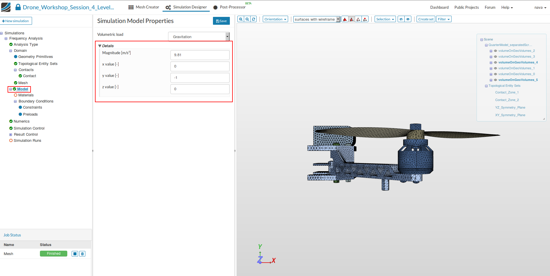
Model
Next we have to define the physical model we want to use for this simulation.
-
Click therefore on the Model item in the project tree which will open a middle column windows. Here you can define the gravitation.
-
Specify the following parameters:
- Magnitude: 9.81
- x value: 0
- y value: -1
- z value: 0
Materials
Now we define and assign material properties to the different parts.
- Click on the Material item in the project tree. This will open a middle column menu where you can edit and create materials and assign them to volumes. Click on the New button
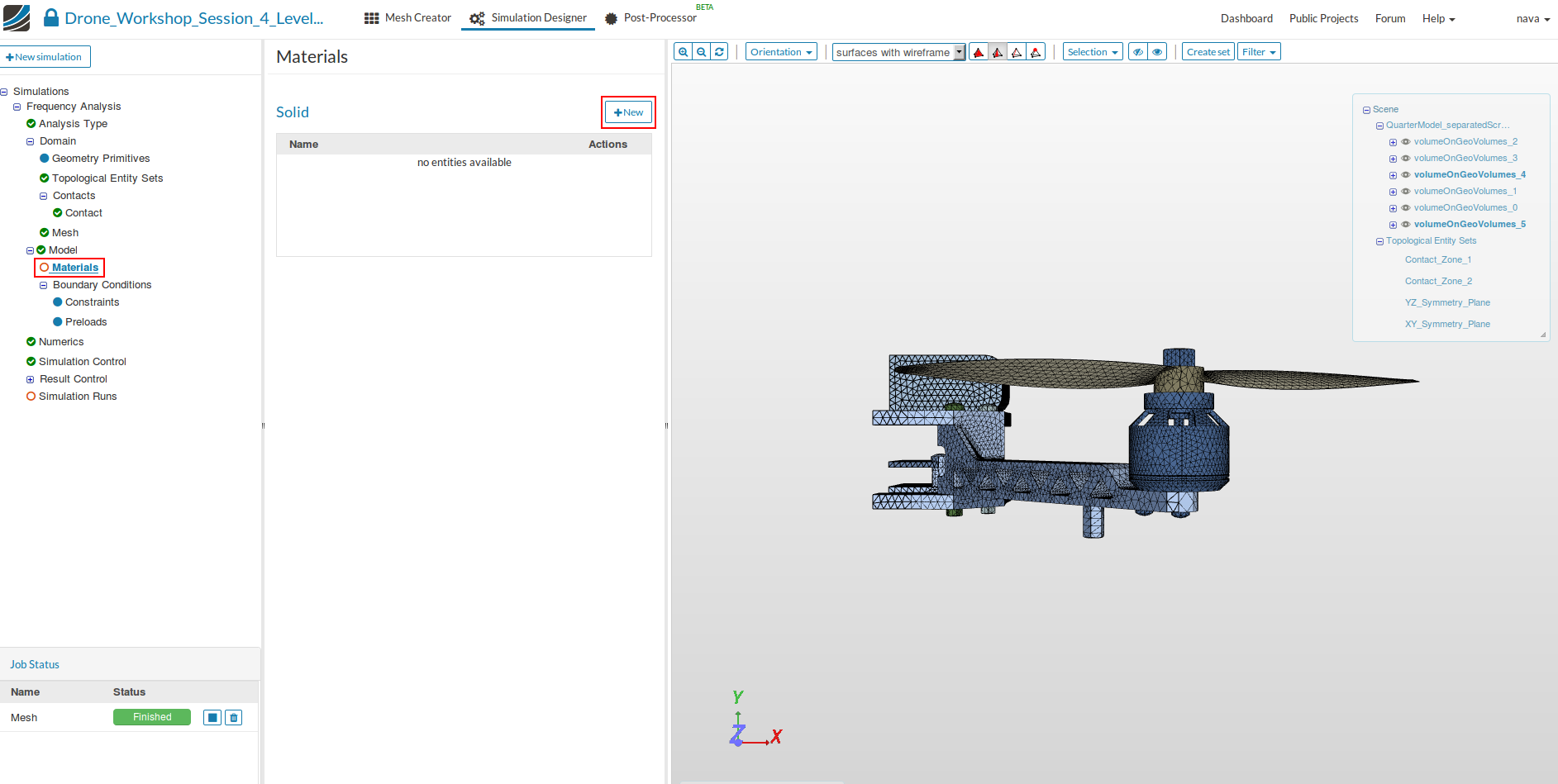
Now you can define your new material based on your own material properties or access our Material Library which includes ready-to-use material models for several materials.
We will start with the manual definition of materials:
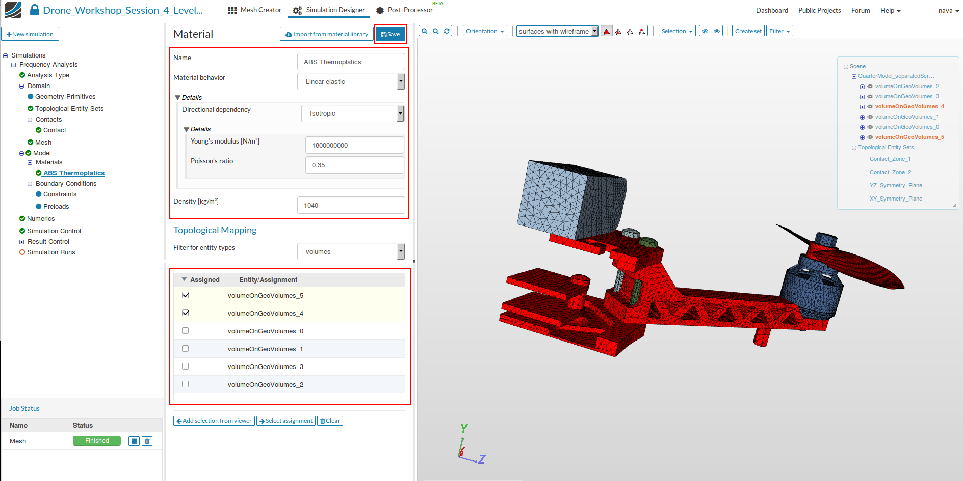
ABS Thermoplastics
- Specify the following parameters:
- Name: ABS Thermoplastic
- Young’s Modulus [N/m2]: 1800000000
- Poisson’s ratio: 0.35
- Density [kg/m3]: 1040
- Assign it to the drone body and the propeller (volumeOnGeoVolumes_4, volumeOnGeoVolumes_5) and finally Save the settings.
- Add an additional material to your project tree for defining the next material.
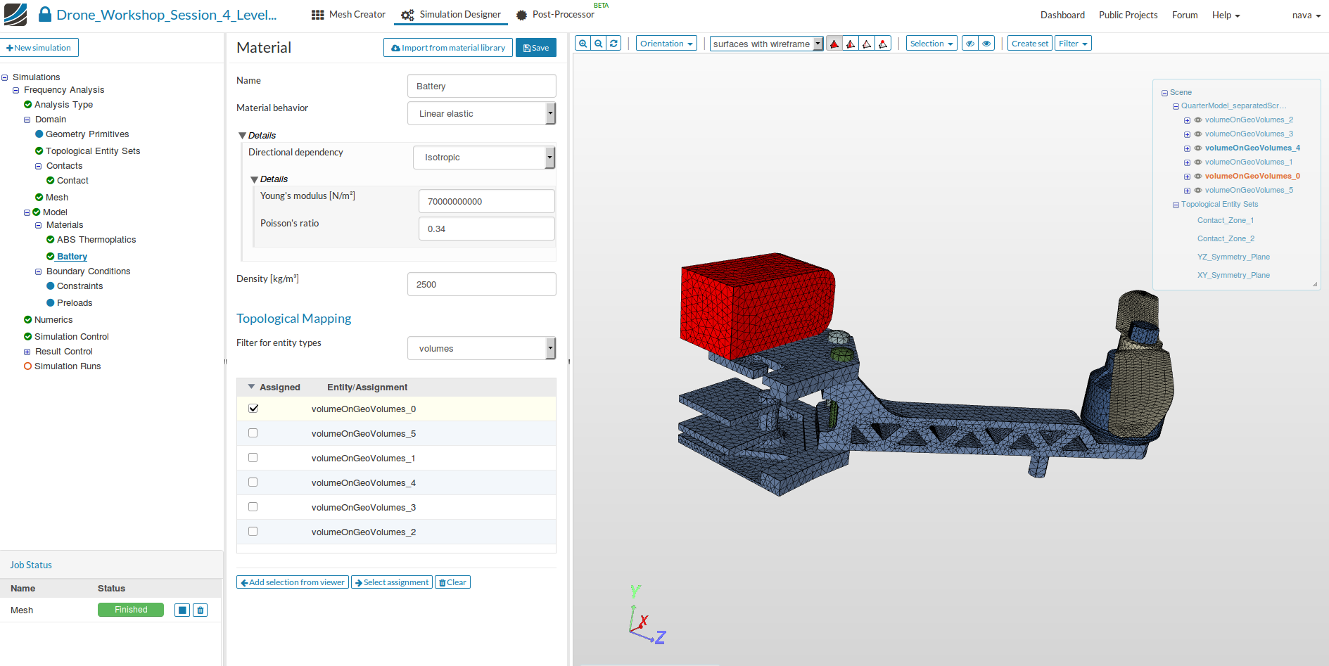
Battery
- Specify the following parameters:
- Name: Battery
- Young’s Modulus [N/m2]: 70000000000
- Poisson’s ratio: 0.34
- Density [kg/m3]: 2500
- Assign the material to the battery of the drone (volumeOnGeoVolumes_0)and finally Save the settings.
Steel
Next we will assign the steel material model to the screws and the engine. Add an additional material to your project tree.
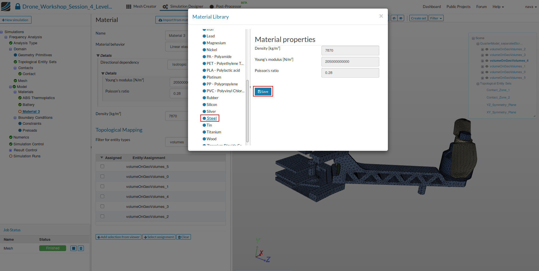
Now we will access our material library instead of creating the material model manually.
- Click on the Import from material library which will open a widget.
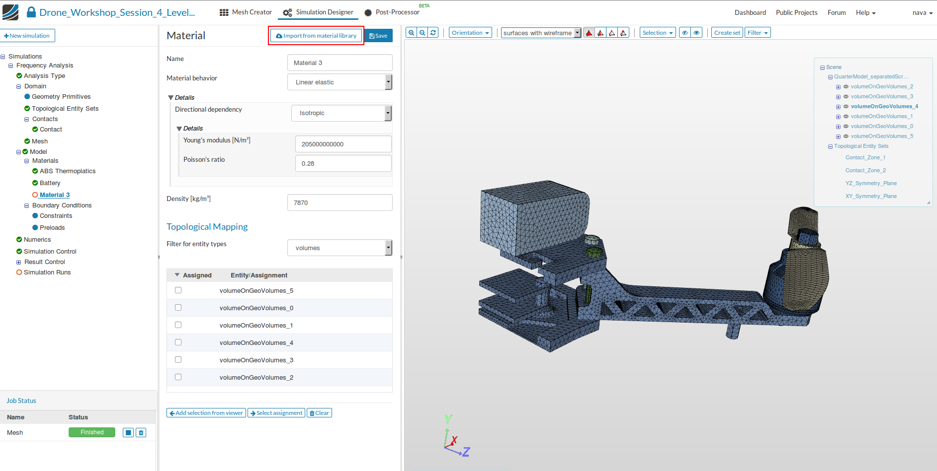
- Please select steel from the list on the left side and save your selection by clicking the related button.
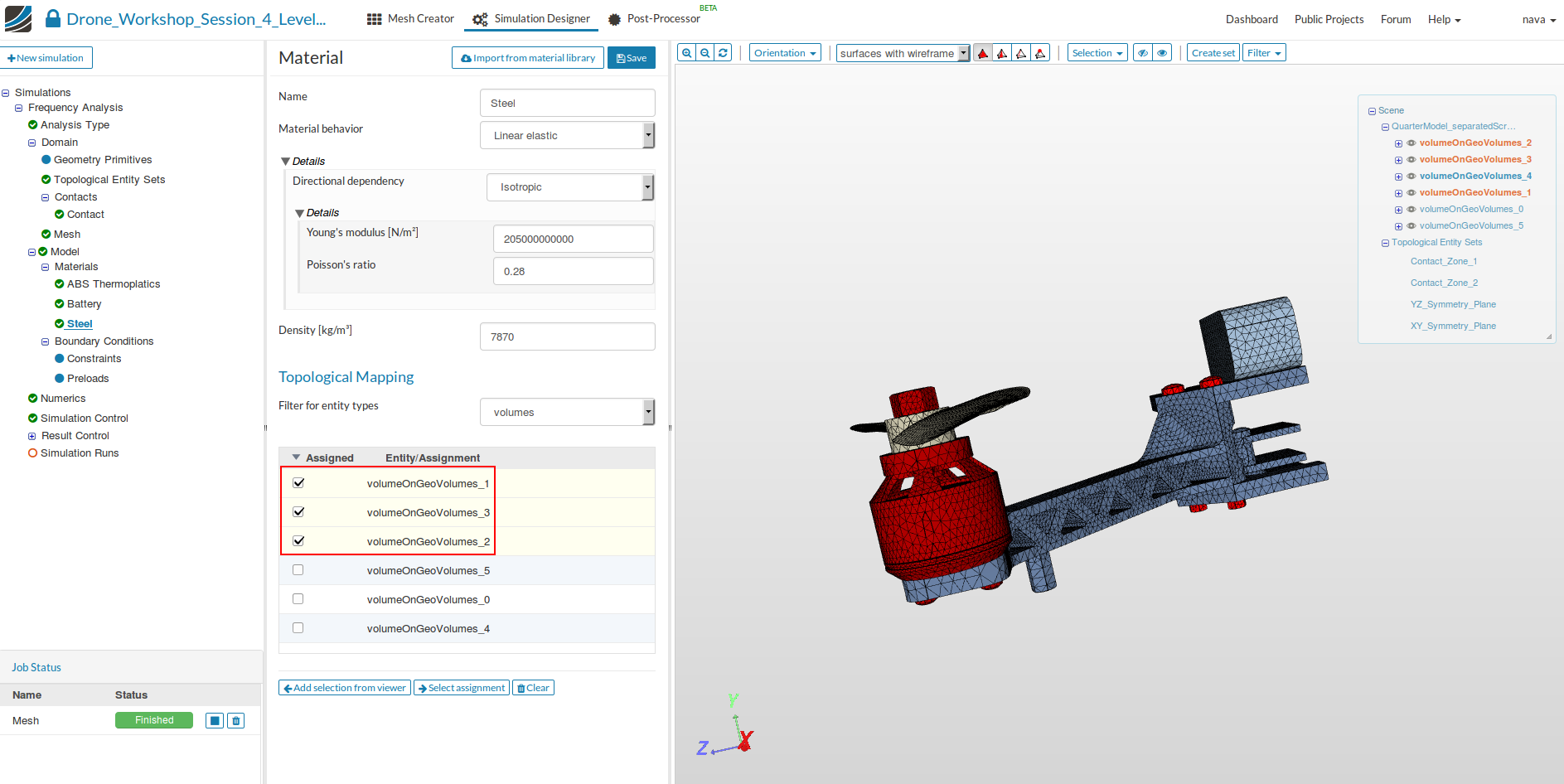
- Now assign the material to the screws and the engine (volumeOnGeoVolumes_1, volumeOnGeoVolumes_2, volumeOnGeoVolumes_3).
Boundary Conditions
Next we can start to define the boundary conditions.
There are two kinds of boundary conditions for structural simulations.
- Constraint conditions are used to limit the degrees of freedom of the model.
- Load conditions are applying an external load to the model
Due the fact that this is only a frequency analysis we only need to define two constraint boundary conditions (external loads are not important at this stage)
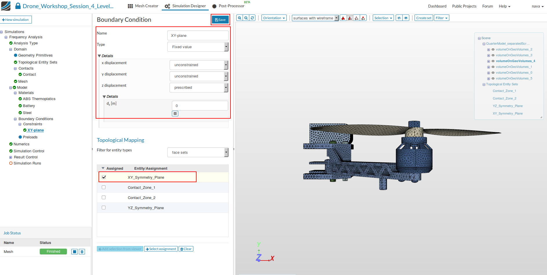
Symmetry XY-plane
This boundary condition is required because we are using a quarter model of the drone.
-
Create a new constraint boundary condition by first clicking on the Constraint and then on New button.
-
Specify the following parameters:
- Name: Symmetry XY-plane
- Type: Fixed Value
- x displacement: unconstrained
- y displacement: unconstrained
- z displacement: prescribed with a value of 0
- Finally, assign the boundary condition to the face set XY_Symmetry_Plane and then Save.
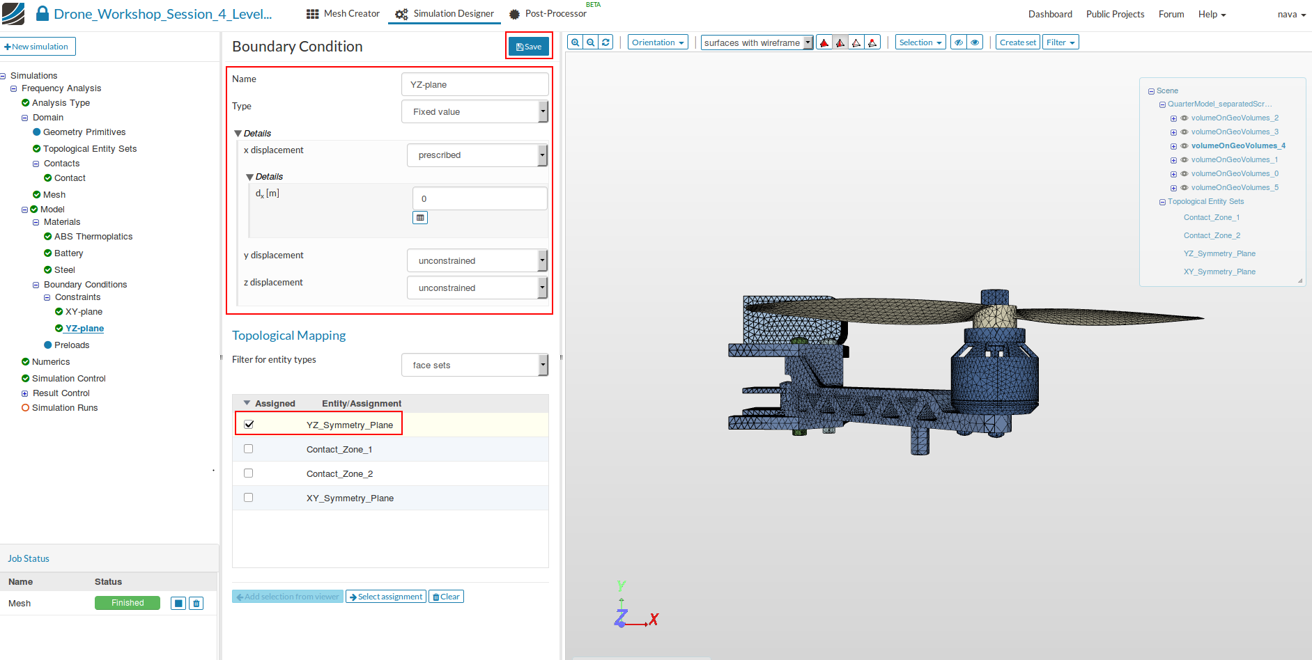
Symmetry YZ-plane
This boundary condition is required because we are using a quarter model of the drone.
- Create a new constraint boundary condition same as above.
- Specify the following parameters:
- Name: Symmetry YZ-plane
- Type: Fixed Value
- x displacement: prescribed with a value of 0
- y displacement: unconstrained
- z displacement: unconstrained
- Finally, assign the boundary condition to the face set YZ_Symmetry_Plane and then Save.
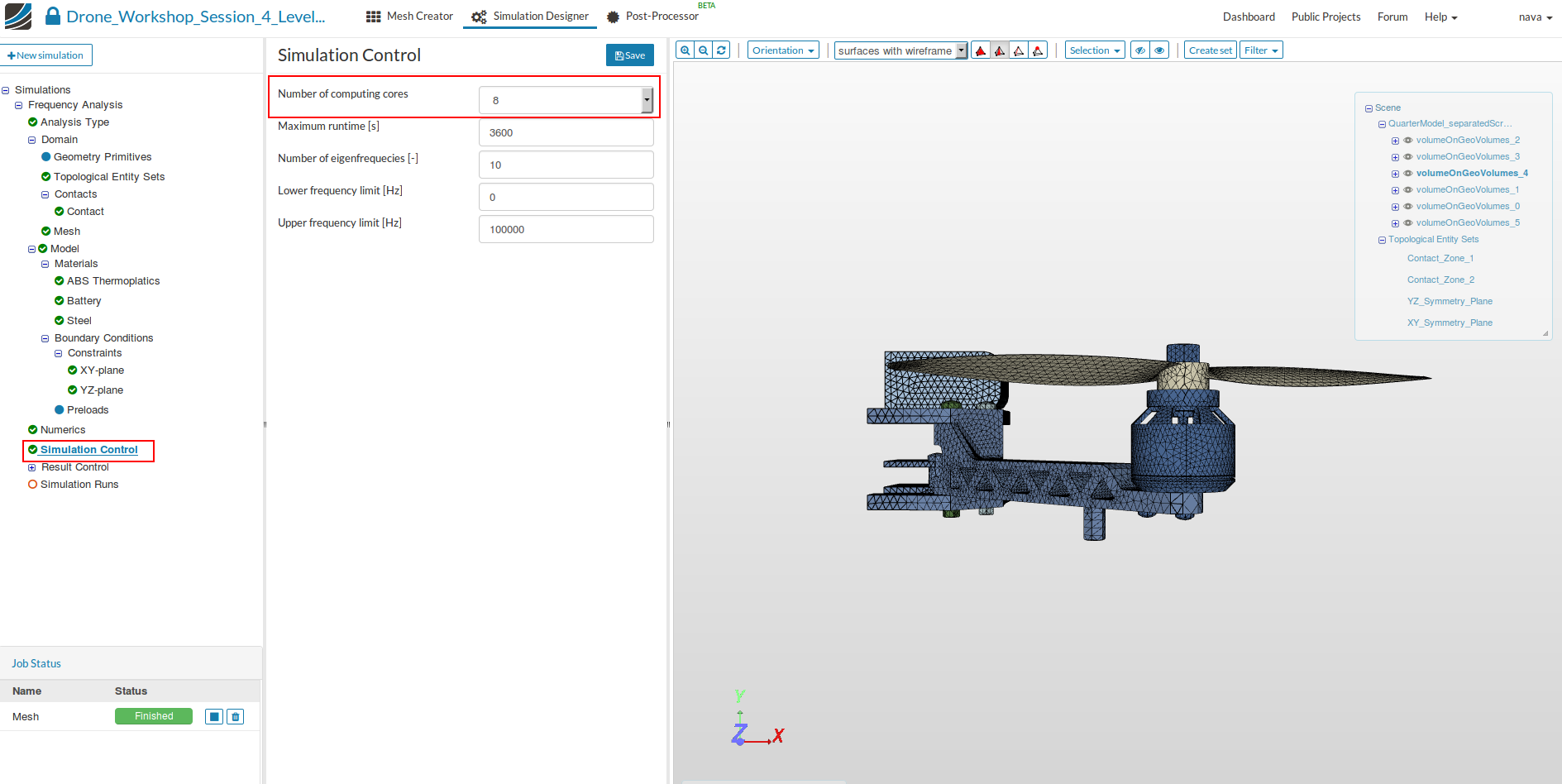
Numerics and Simulation Control
Numerics, which is the next item in the project tree, can be skipped since the default settings are fine.
Click on the Simulation Control item in the project tree to specify how fast and accurate you want the simulation to be computed and change the Number of computing cores to 8 in order to accelerate the simulation.
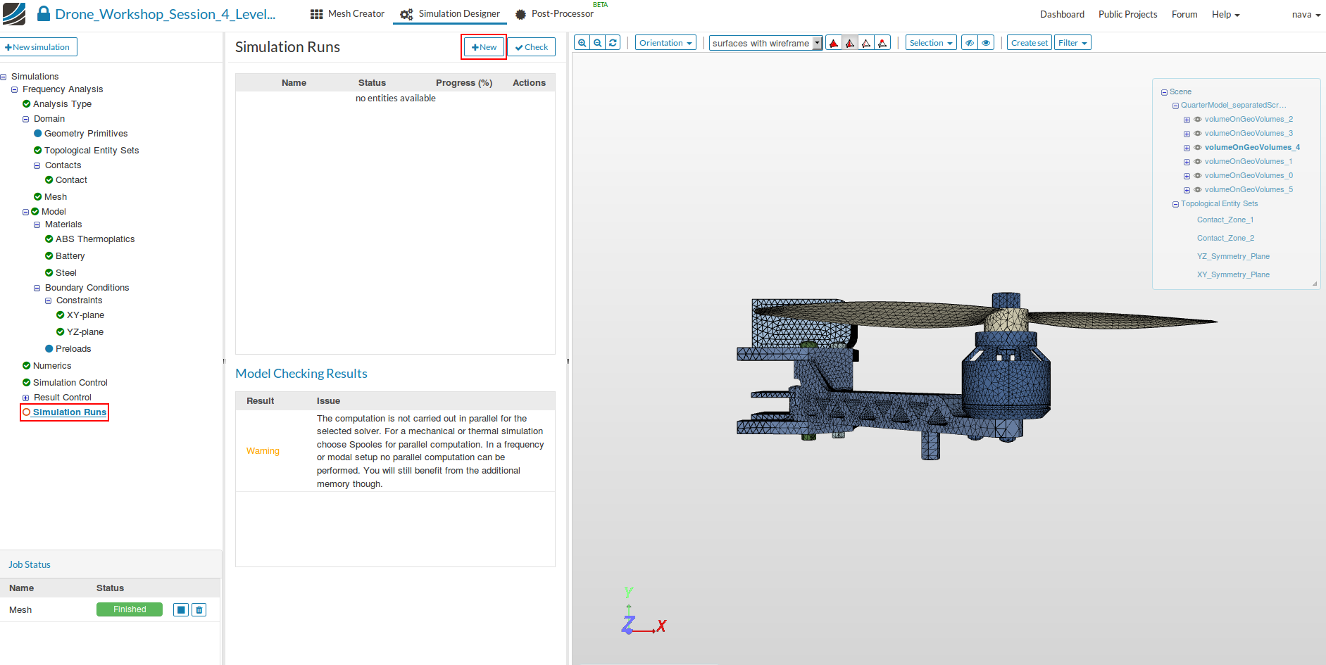
Simulation Runs
- To start the simulation, click on the Simulation Runs item in the tree and click on the New button at the top of the middle column menu. This will create a snapshot of your simulation settings as a new sub-item.
- You can now start the simulation run by selecting it from the project tree and then click on the Start button.
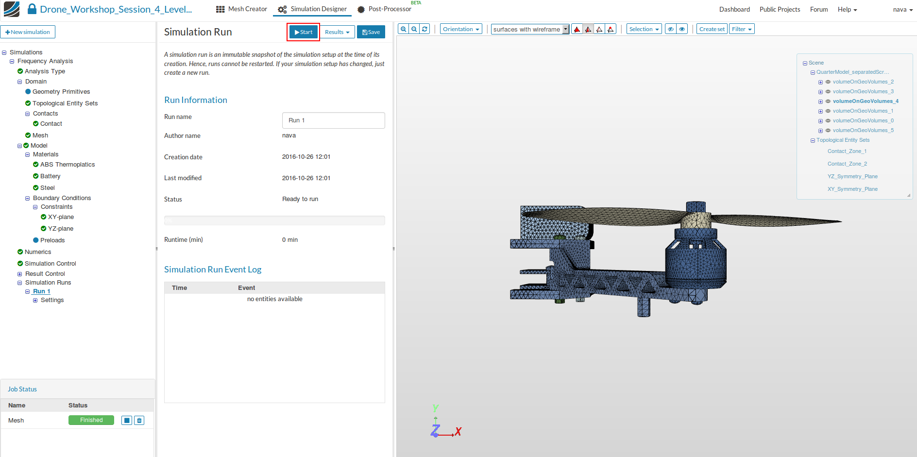
Once your simulation is finished, please click on the Post-Processor button in the main ribbon bar.
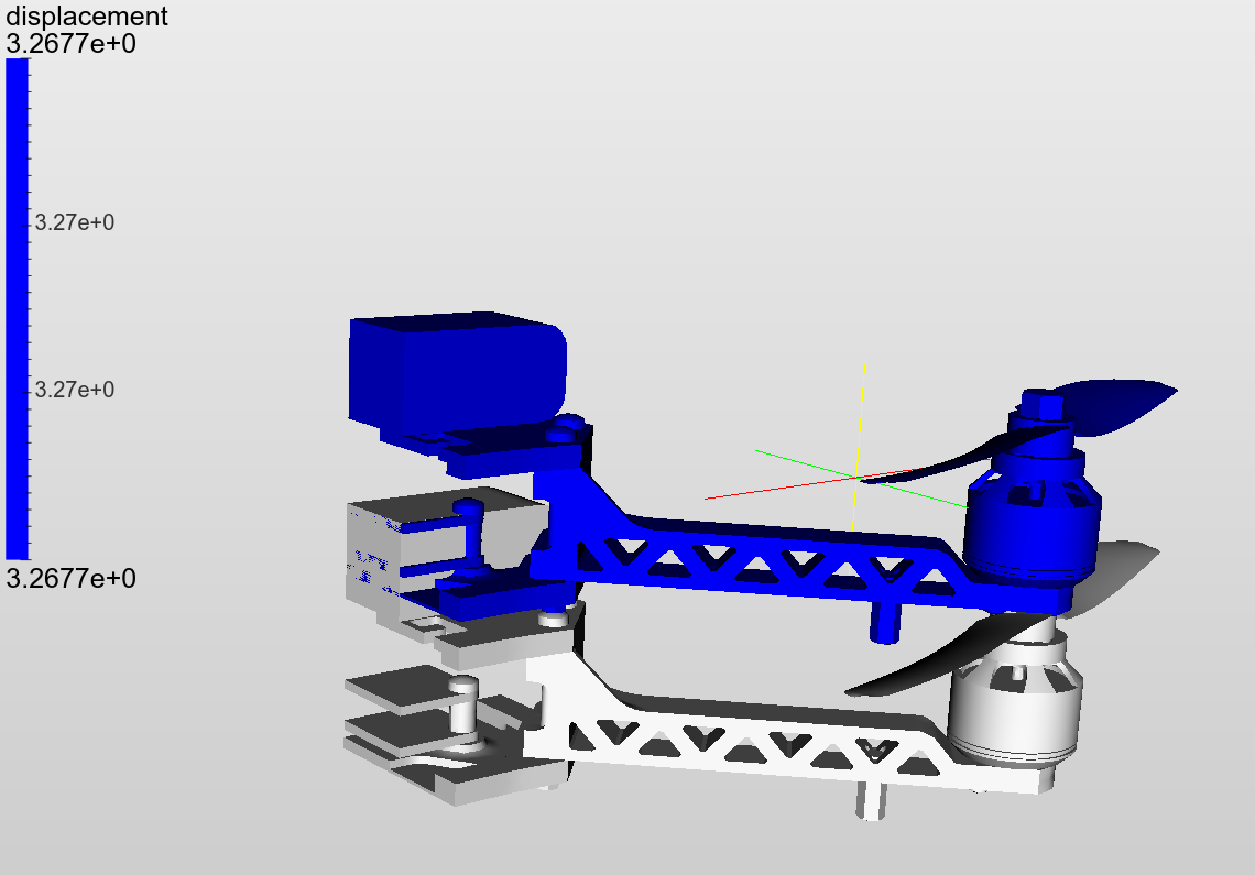
Post Processing
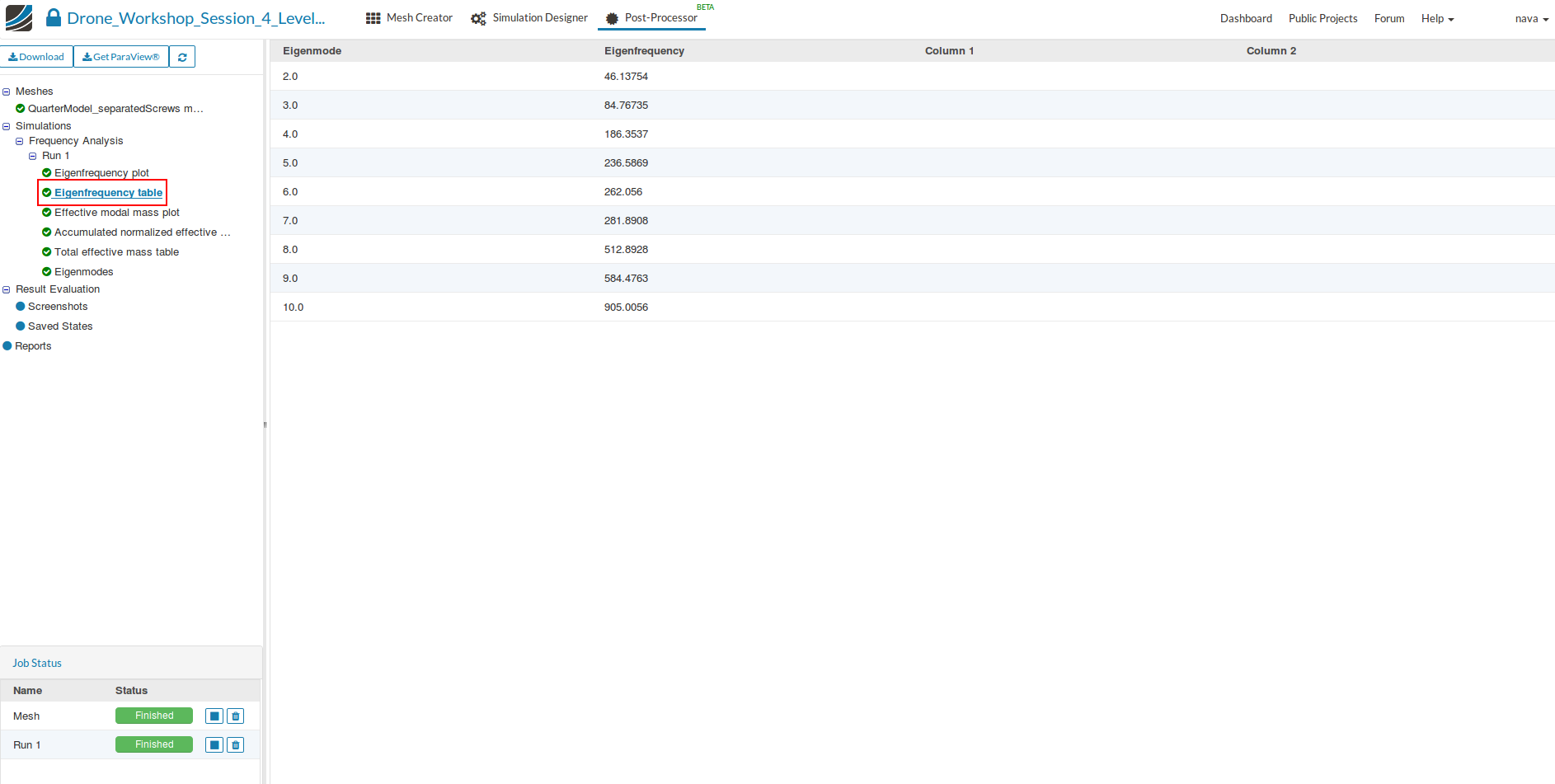
Now we will take a look at the results of our simulation. Since we are interested to find out the eigenfrequencies of the drone, we will not perform a 3D post processing.
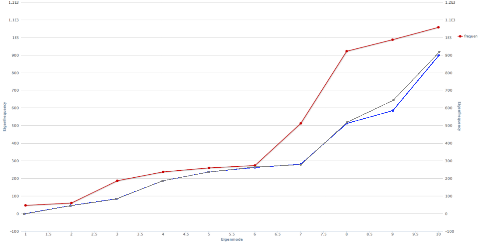
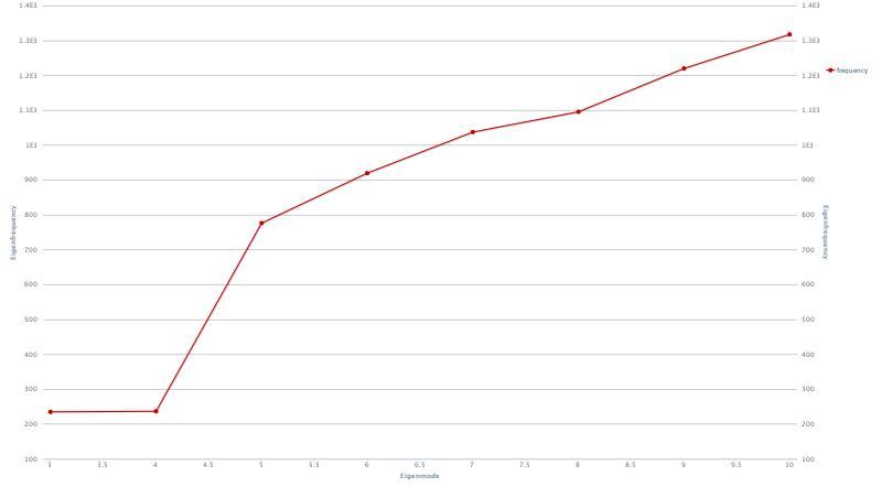
Please click on the Eigenfrequency plot sub-item in the project tree. This will open a graph which shows the first 10 eigenmodes and the related eigenfrequency.
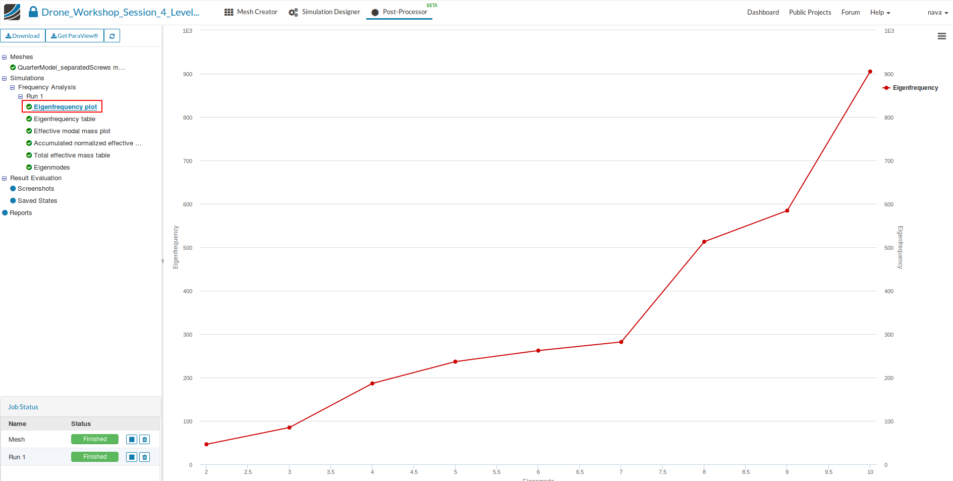
You can also access a table with the eigenfrequencies by clicking the Eigenfrequency table item in the project tree.