Rotating Zones
Now we will create MRF zones, go ahead and add a Rotating Zone under Advanced Concepts. Rename it to Front wheel MRF
Then change:
-
Origin x value [m], y value [m] and z value [m] value to -0.41566, 0.670378 and 0.219731 respectively.
-
Axis of rotation y value [m] to 1
-
Angular velocity [rad/s] to -90.9
-
Then select FrontWheelZone under Topological Mapping and click Select assignment in order to see the selected item in the viewer.
-
Click Save to register your changes.

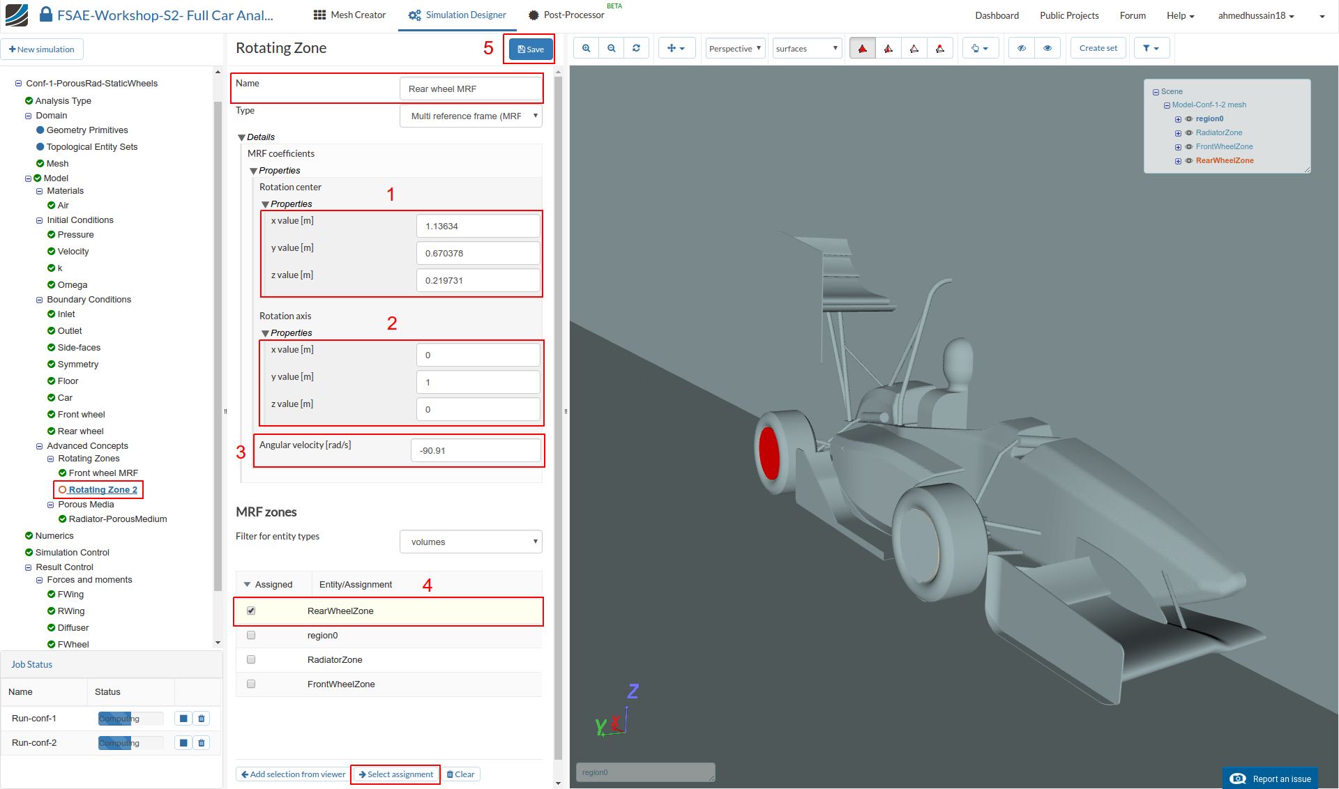
Similarly, perform the same procedure and create a new Rotating Zone. Rename it to Rear wheel MRF. Then change:
-
Rotation center x value [m], y value [m] and z value [m] value to 1.13634, 0.670378 and 0.219731 respectively.
-
Rotation axis y value [m] to 1.
-
Angular velocity [rad/s] to -90.9
-
Then select RearWheelZone under MRF zones and click Select assignment in order to see the selected item in the viewer.
-
Click Save to register your changes.
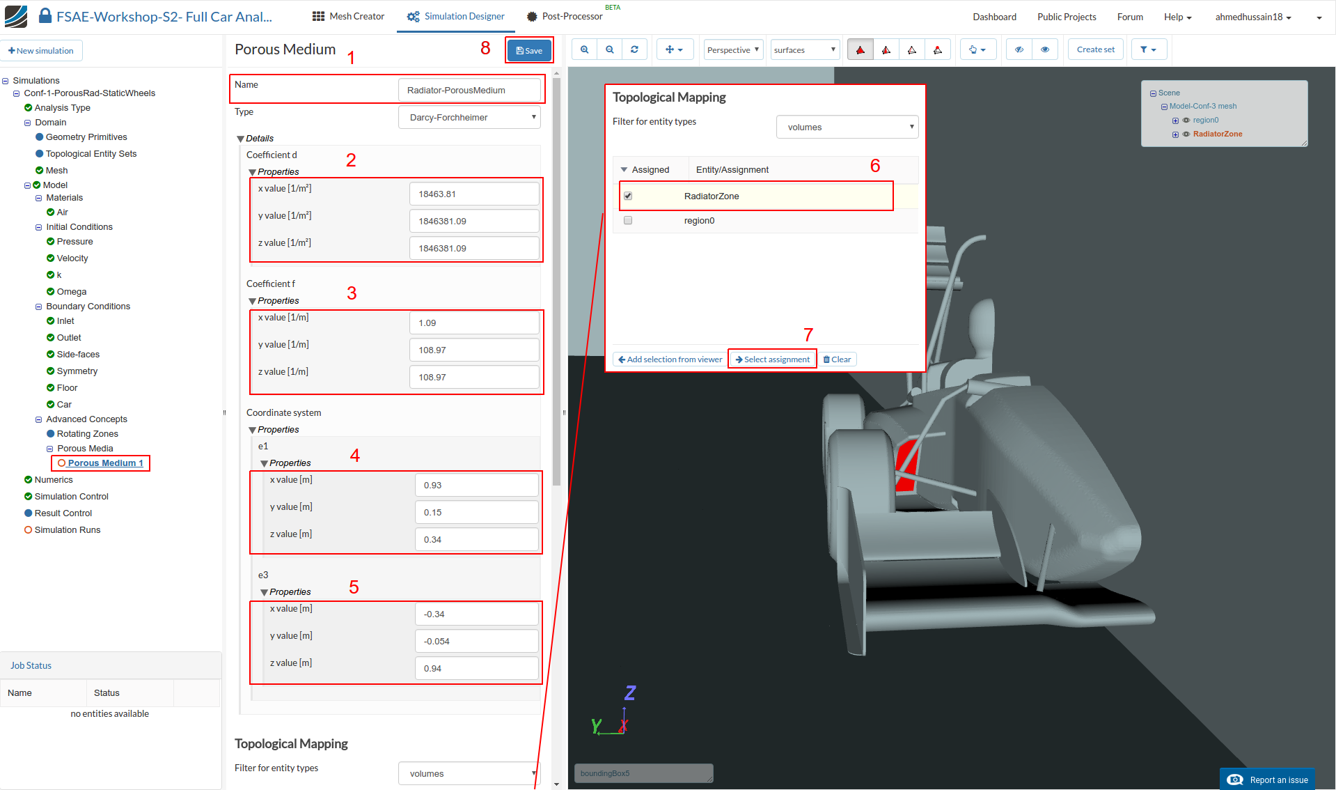
Porous Media
In this section we will define the radiator volume source via porous media. Expand the Advanced Concepts tree item and proceed to Porous Media. Click +New to create a new porous media definition.

After creating a new porous media definition, you will be automatically directed to the its properties panel. Change:
-
Name to Radiator-PorousMedium (optional) and set the Type to Darcy-Forchheimer
-
Coefficient d x, y and z values to 18463.81, 1846381.09 and 1846381.09 respectively.
-
Coefficient f x, y and z values to 1.09, 108.97 and 108.97 respectively.
-
Coordinate system e1 x, y and z values to 0.93, 0.15 and 0.34 respectively.
-
Coordinate system e3 x, y and z values to -0.34, -0.054 and 0.94 respectively.
-
Scroll down and select RadiatorZone under Topological Mapping.
-
Click Select assignment to see the selected volume source in viewer.
-
Click Save to register your changes.
Numerics
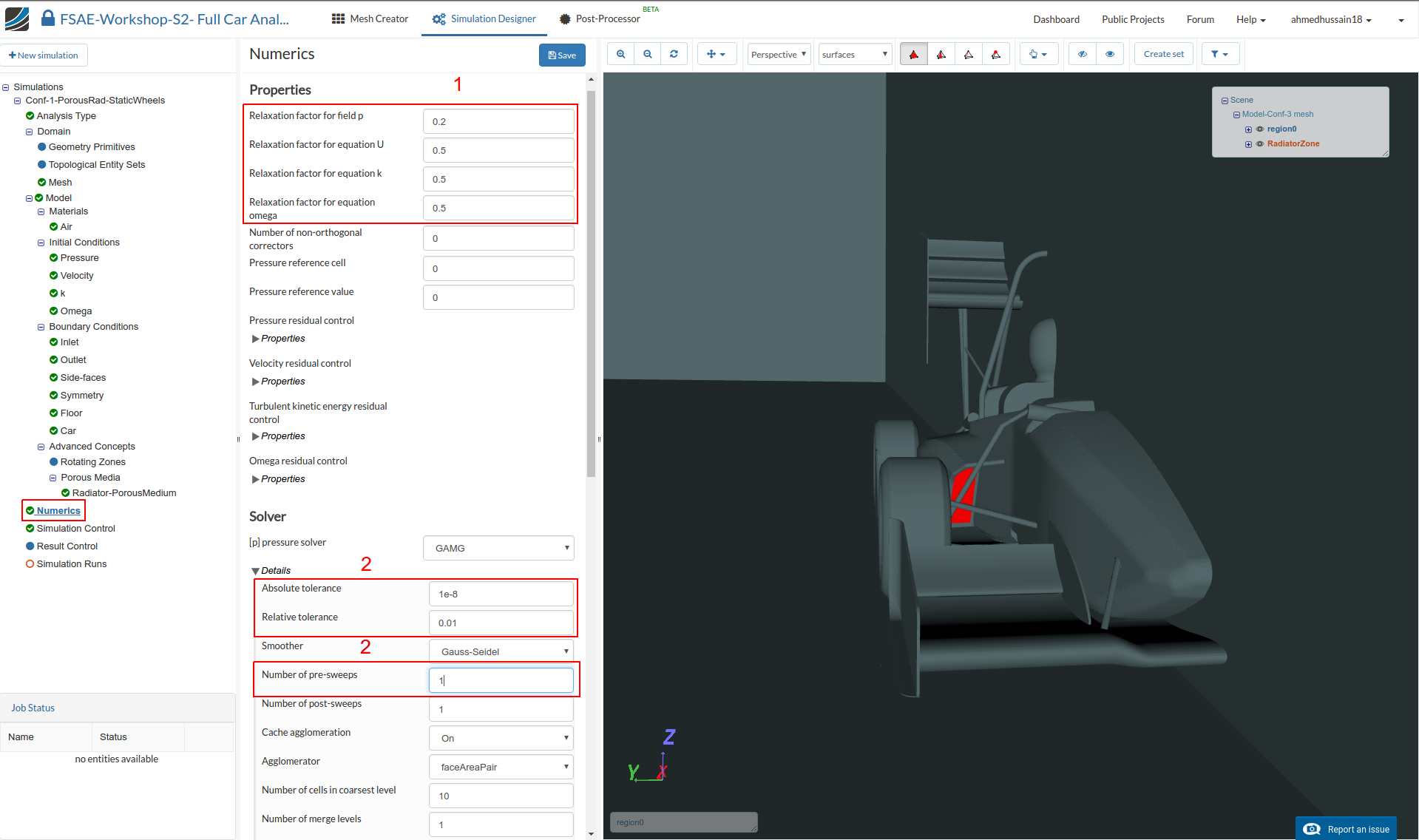
After defining all the boundary conditions, we will proceed to set up the numerics for our simulation. Go to Numerics and change:
-
Relaxation factor for field p, Relaxation factor for equation U, Relaxation factor for equation k and Relaxation factor for equation omega to 0.2, 0.5, 0.5 and 0.5 respectively.
-
Furthermore, under [p] pressure solver, change Absolute tolerance, Relative tolerance and Number of pre-sweeps to 1e-8, 0.01 and 1 respectively.
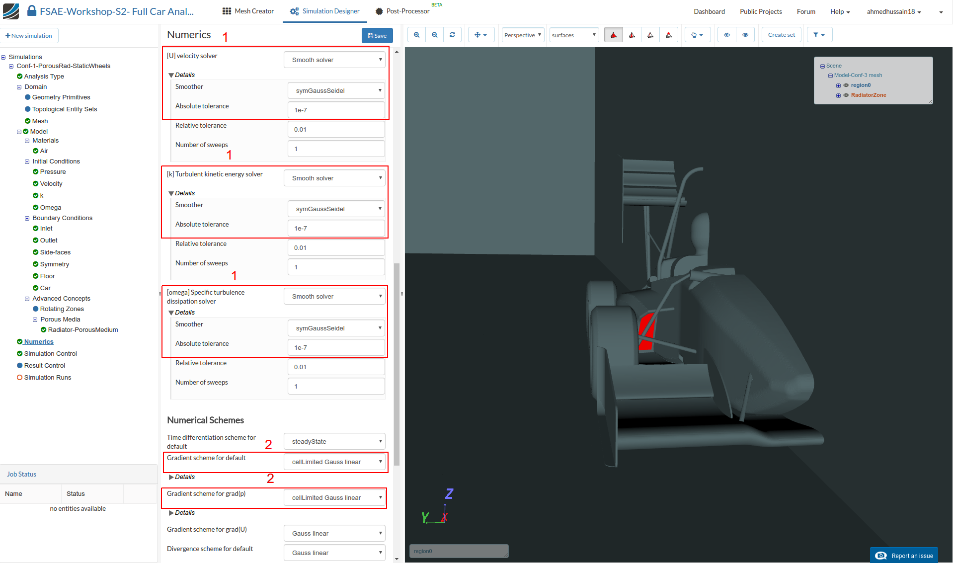
Scroll down until [U] velocity solver and change:
-
[U] velocity solver to Smooth solver, Smoother to symGaussSeidel and Absolute tolerance to 1e-7. Do the same for [k] Turbulent kinetic energy solver and [omega] Specific turbulence dissipation solver.
-
Change both Gradient scheme for default and Gradient scheme for grad(p) to cellLimited Gauss linear
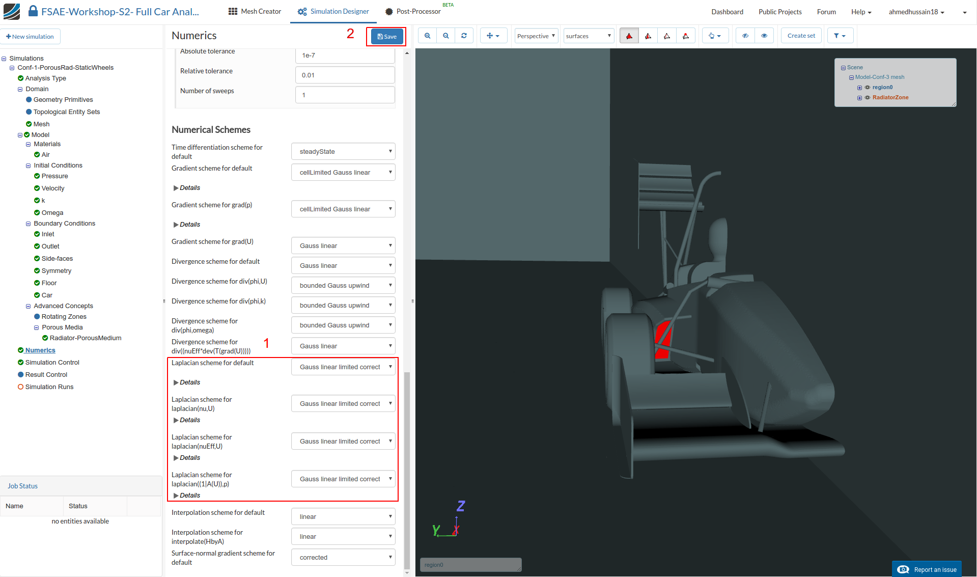
Scroll down to the end and change:
-
Laplacian scheme for default, Laplacian scheme for laplacian(nu,U), Laplacian scheme for laplacian(nuEff,U) and Laplacian scheme for laplacian((1|A(U)),p) to Gauss linear limited corrected
-
Click Save to register all of your changes.
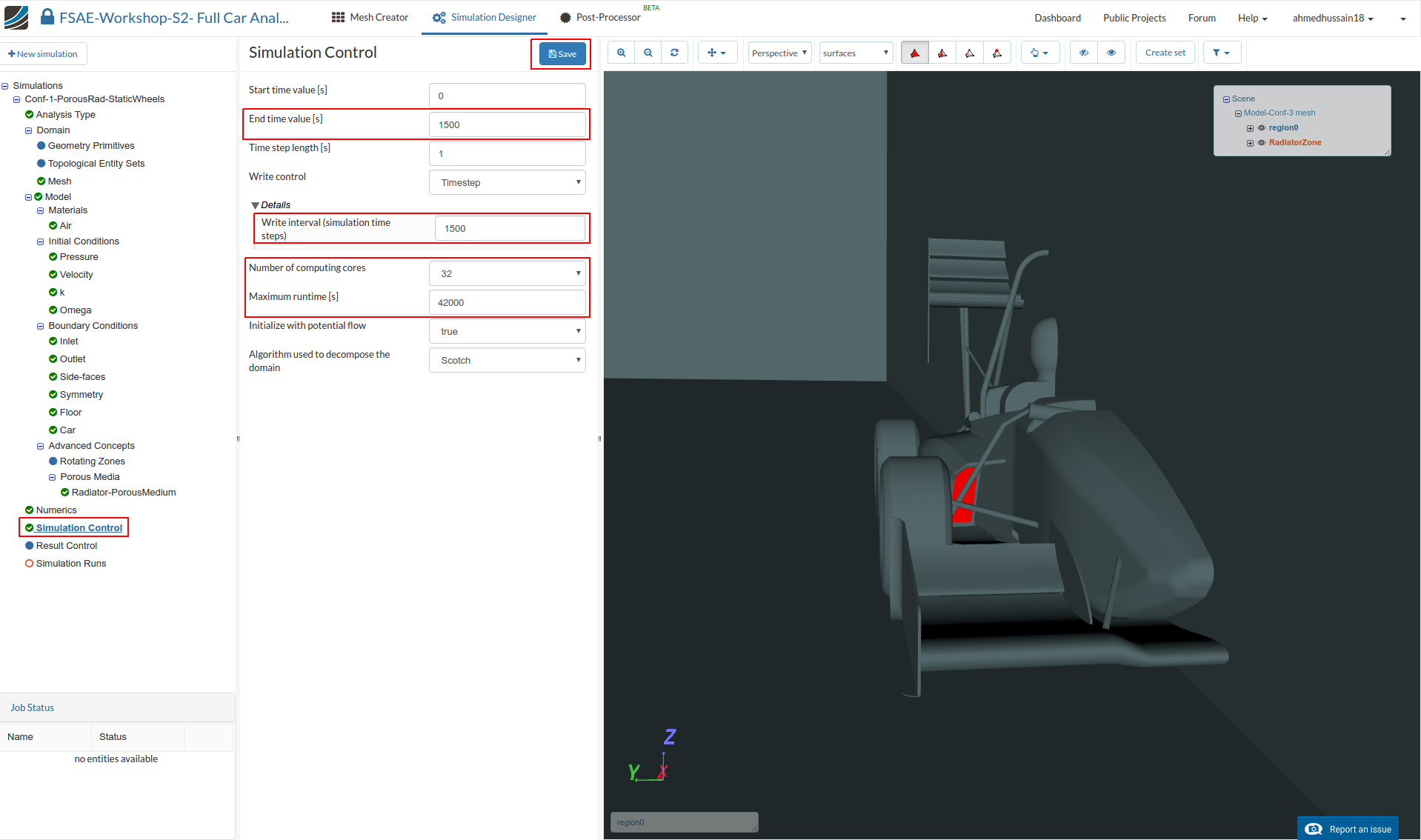
Simulation Control
Next we will define our simulation interval and steps that needs to be recorded. Go to Simulation Control and change End time value [s] to 1500.
Expand Details under Write control and change Write interval (simulation time steps) to 1500.
Next change Number of computing cores and Maximum runtime [s] to 32 and 42000 respectively.
Click Save to register your changes.
Result Control
As our last step before running the simulation, we will create result control items in order to get graphical data sets of interest. Firstly, we will create the result control item for the forces and moments.
Go to Result Control and click New next to Forces and Moments.

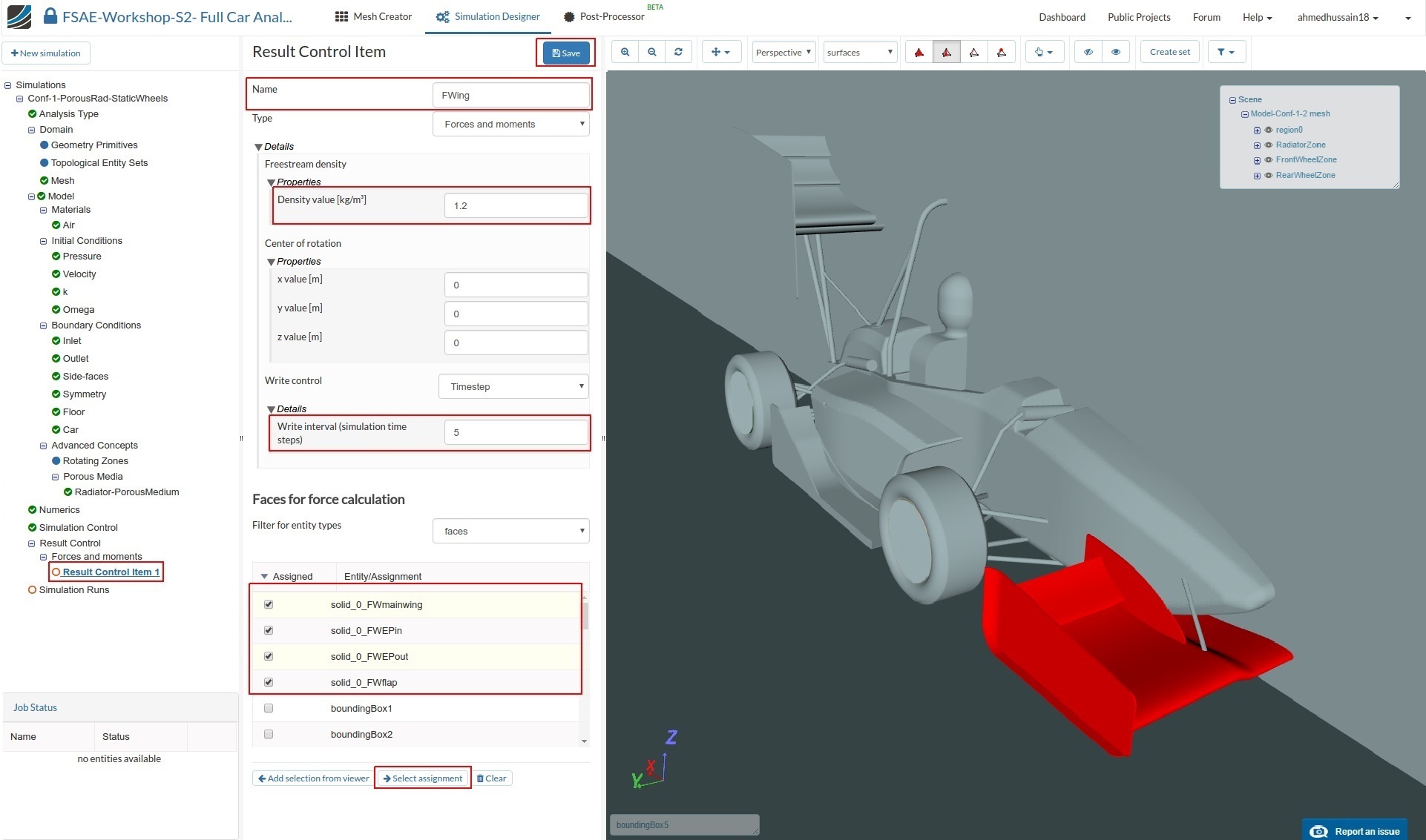
A new force and moment result control item will be created. Rename it to FWing (optional).
Then change Density value [kg/m³] and Write interval (simulation time steps) to 1.2 and 5 respectively.
Select solid_0_FWmainwing, solid_0_FWEPin, solid_0_FWEPout and solid_0_FWflap under Faces for force calculation.
Click Select assignment to see the selected regions in the viewer and then click Save to register your changes.
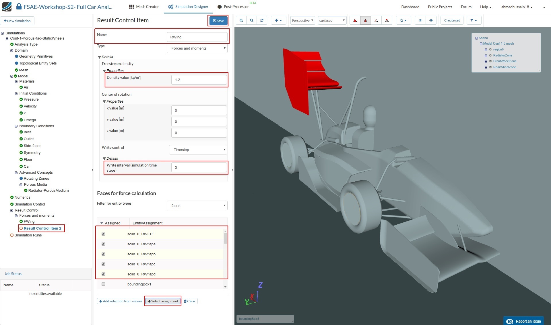
Create another force and moment result control item and rename it to RWing (optional).
Then change Density value [kg/m³] and Write interval (simulation time steps) to 1.2 and 5 respectively.
Select solid_0_RWEP, solid_0_RWflapa, solid_0_RWflapb, solid_0_RWflapc and solid_0_RWflapd under Faces for force calculation.
Click Select assignment to see the selected regions in the viewer and then click Save to register your changes.
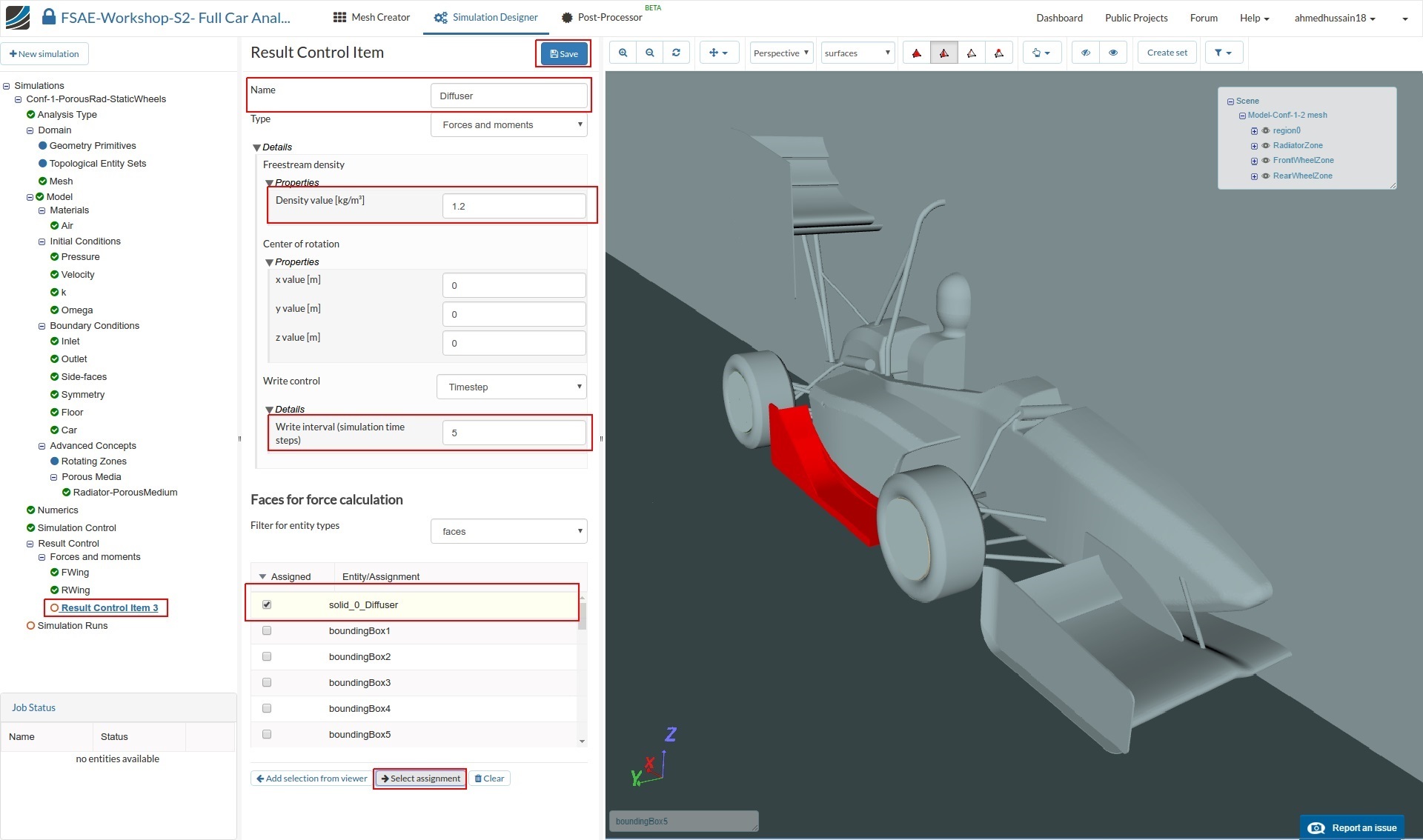
Follow the same procedure to create force and moment result control item for the diffuser. Rename it to Diffuser (optional).
Then change Density value [kg/m³] and Write interval (simulation time steps) to 1.2 and 5 respectively.
Select solid_0_Diffuser under Faces for force calculation.
Click Select assignment to see the selected regions in the viewer and then click Save to register your changes.
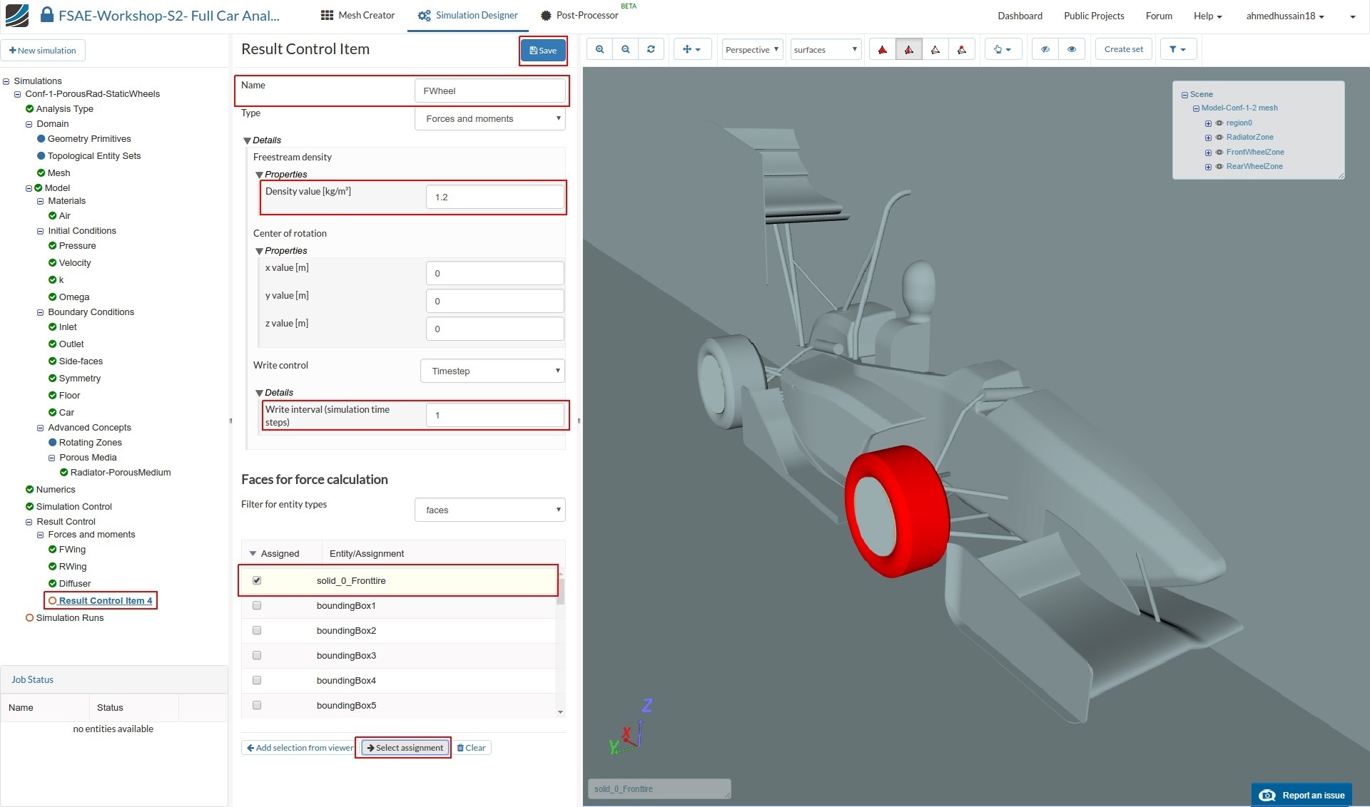
Follow the same procedure to create force and moment result control item for the front wheel and rename the newly created result control item to FWheel (optional).
Then change Density value [kg/m³] and Write interval (simulation time steps) to 1.2 and 5 respectively.
Select solid_0_Fronttire under Faces for force calculation.
Click Select assignment to see the selected regions in the viewer and then click Save to register your changes.
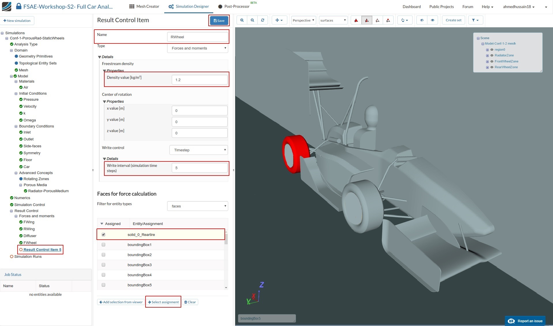
Do the same for rear wheel, rename it to RWheel (optional).
Then change Density value [kg/m³] and Write interval (simulation time steps) to 1.2 and 5 respectively.
Select solid_0_Reartire under Faces for force calculation.
Click Select assignment to see the selected regions in the viewer and then click Save to register your changes.
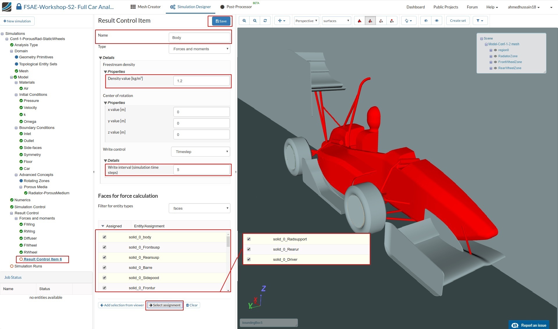
Similarly, for the whole body repeat the procedure and this time rename it to Body (optional).
Then change Density value [kg/m³] and Write interval (simulation time steps) to 1.2 and 5 respectively.
Select solid_0_body, solid_0_Frontsusp, solid_0_Rearsusp, solid_0_Barre, solid_0_Sidepood, solid_0_Frontur, solid_0_Radsupport, solid_0_Rearur and solid_0_Driver.
Click Select assignment to see the selected regions in the viewer and then click Save to register your changes.
Simulation Run
Once all the above steps are defined, we will proceed to create our first simulation run. Go to Simulation Runs and click on New and then Create in order to create a new run.
After the run is created, click Start to start the created run. The simulation run can take up to ~185 minutes (~3 hrs.)
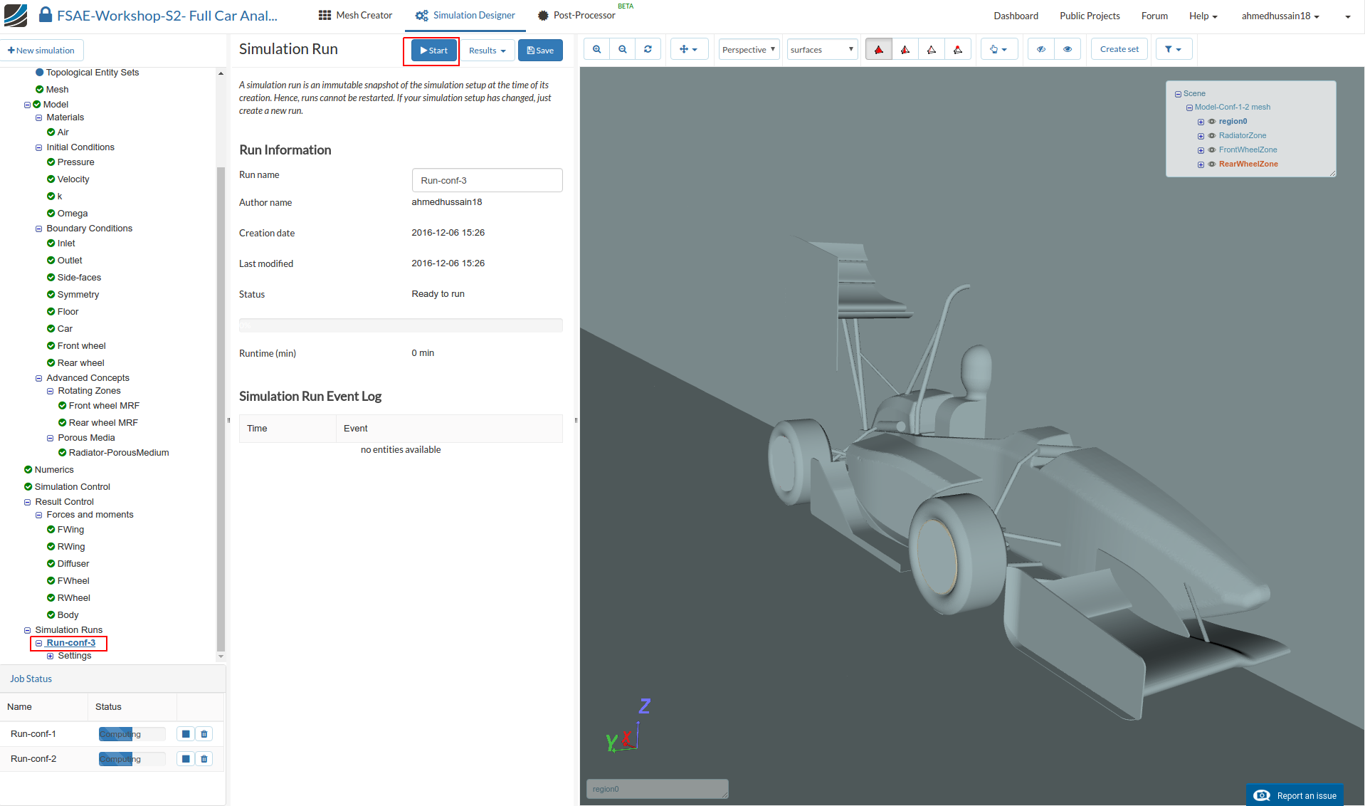
Once your simulation is completed, proceed to Post-Processor tab in order to post-process your results.
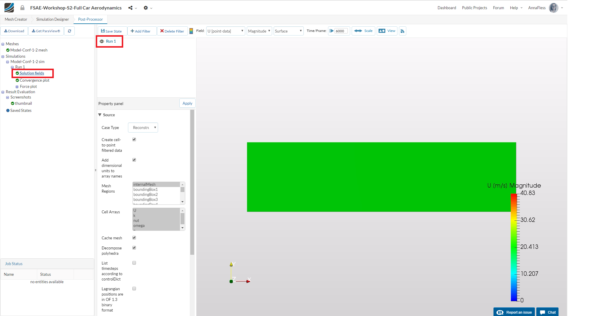
Post-processing
Once in Post-Processor, click on Solution fields under Model-Conf-1-2 sim in order to load the results in viewer. Due to fine mesh it can take up to 5 minutes to load the results in to the viewer.
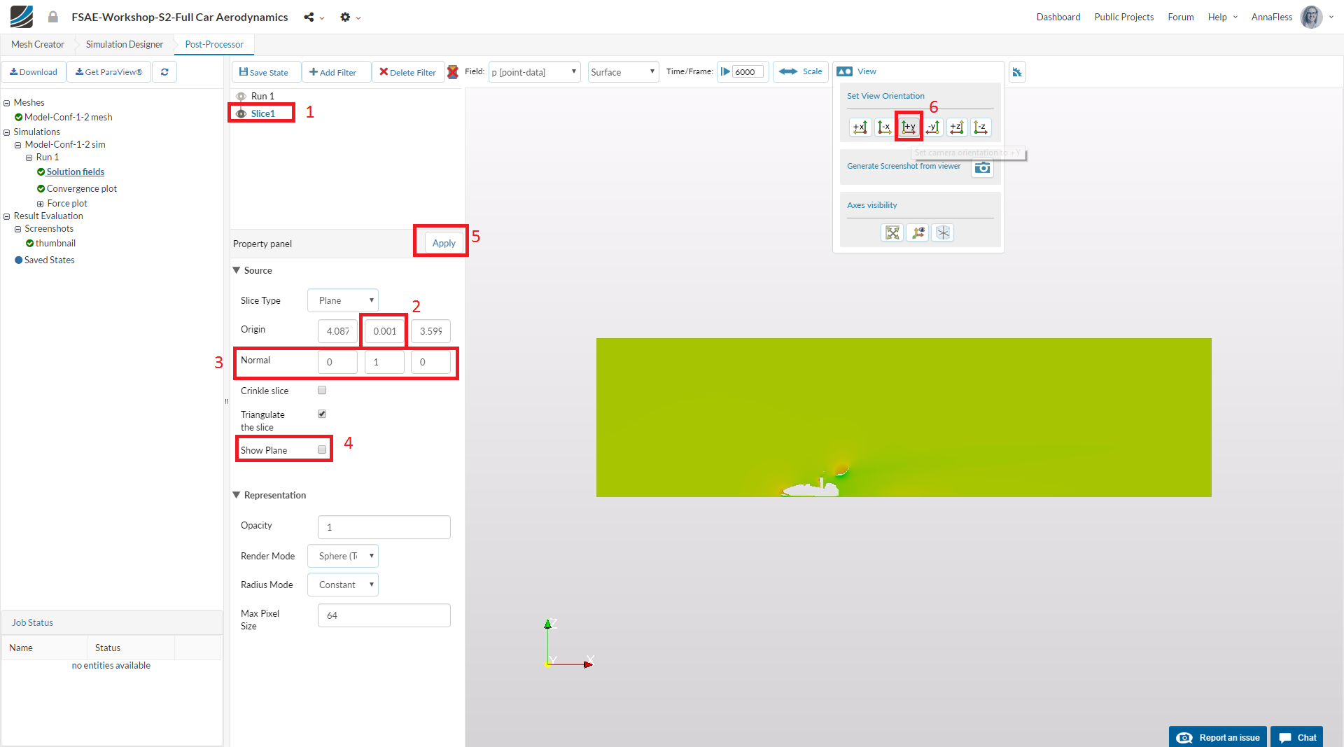
For faster and efficient reviewing of the results, we will use slice filter. In order to add the filter, do the following:
-
Go to Add Filter and select Slice.
-
Change Origin middle value i.e. y value to 0.0011
-
Change Normal to (0,1,0)
-
Uncheck Show Plane.
-
Click Apply to save the changes.
-
Next set camera orientation to +Y from the View tool over the viewer to get a proper view.
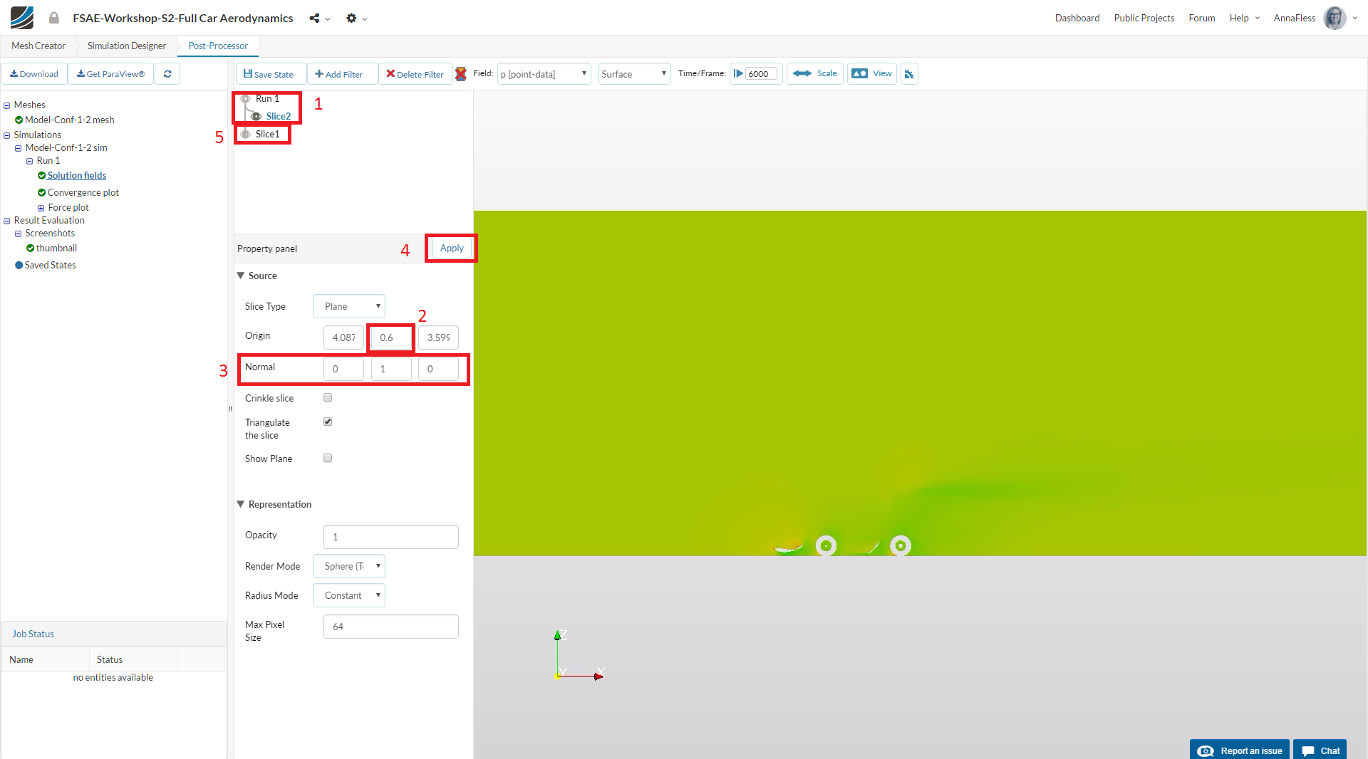
In order to see the pressure and velocity distribution on tires, we have to make another slice. This will be useful afterwards to compare the results between different configurations. First go back to the actual solution field i.e. Run 1 and then:
-
Go to Add Filter and select Slice.
-
Change Origin middle value i.e. y value to 0.6
-
Change Normal to (0,1,0)
-
Click Apply to save the changes.
-
Turn off the previous created slice by unchecking the eye button next to it.
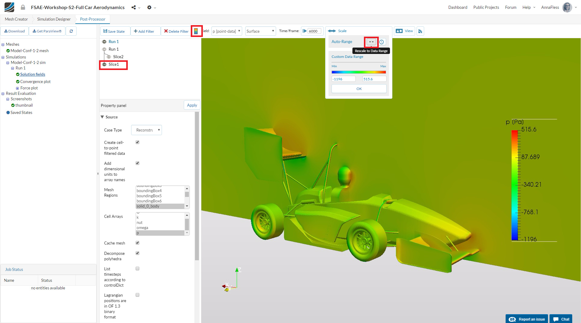
Now we will move further to load the whole car model in order to see the pressure contours over it. For this load again the same result by right clicking on it and then selecting Add result to viewer.
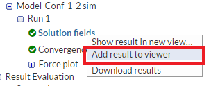
Please note that adding second time the same results can take up to 10 min.
Once the results are loaded, select all the entities next to Mesh Regions starting with solid_0. You can do so by first selecting the first entry i.e. solid_0_body in this case and then holding shift button while going down and then selecting the last one. Next choose only p next to Cell Arrays. Click Apply to save the changes.
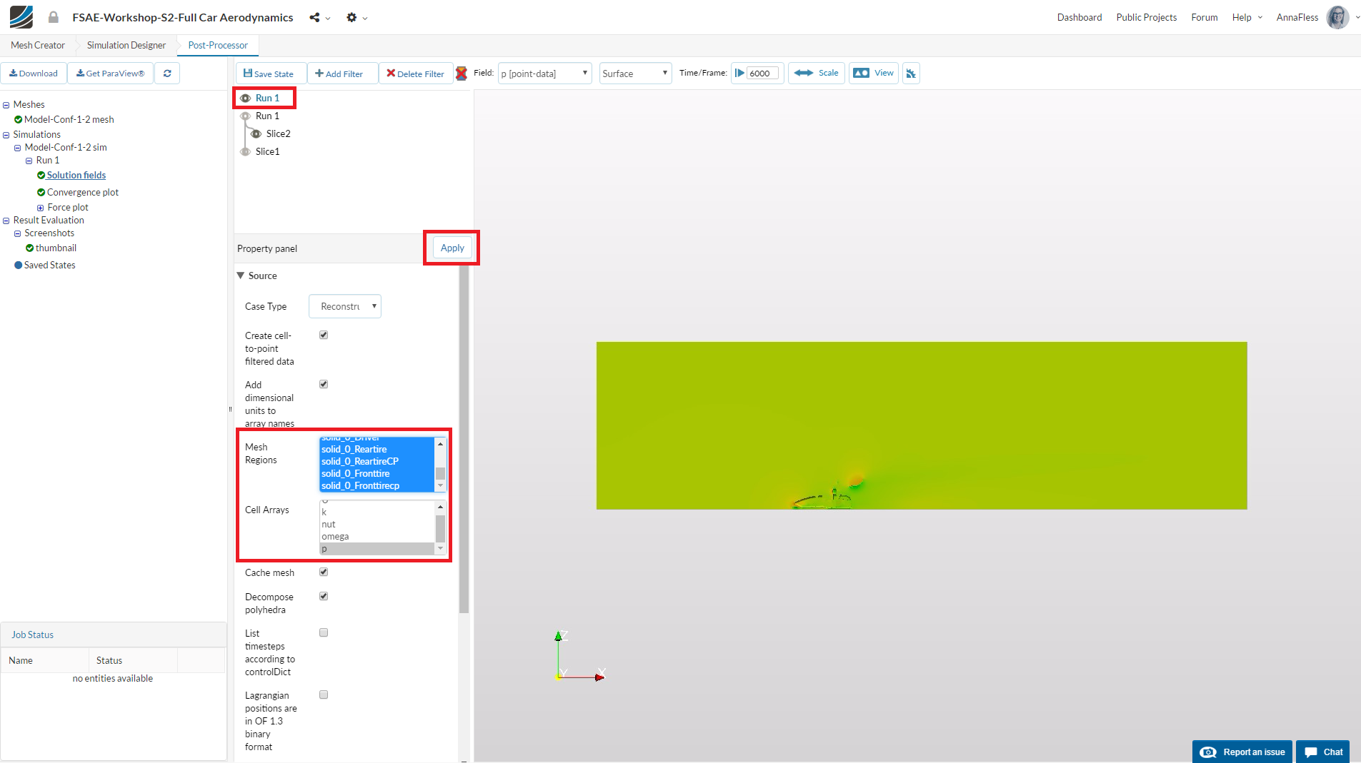
Rescale the pressure contour by clicking the auto rescale button in Scale tool.
Turn on the color bar for pressure and select Slice 1
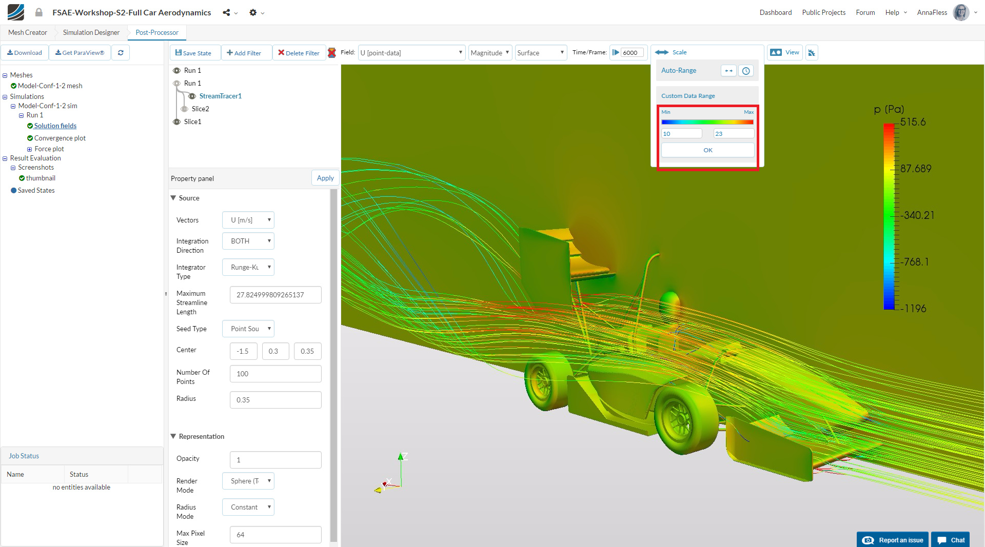
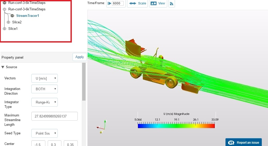
Next we will create the stream lines in order to see the flow.
For this, go back to the first loaded result Run 1
-
Add a filter named StreamTracer
-
Change Center to (-1.5,0.3,0.35)
-
Change Radius to 0.35
-
Click Apply to see the streamlines.
-
Next switch to U [point-data] in order to see the streamlines colored via velocity.
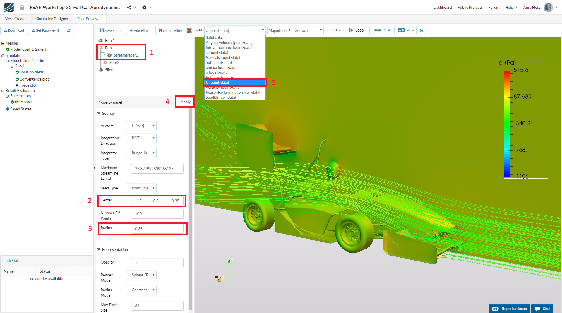
As a last step, we have to rescale the velocity contour to a desired value. To do so, go to the Scale tool and give the lowest and highest values as 10 and 23 respectively. Then click OK. Now also turn on the color bar for the velocity by clicking the color bar button.