Recording

Exercise
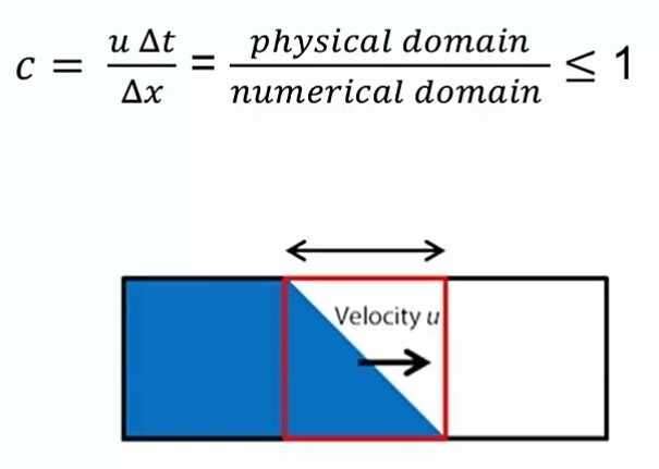
In this exercise we will examine how the Courant number affects the stability and simulation time. A high Courant number speeds up the simulation convergence but can lead to instability. For this reason, the Courant number is restricted below 1 and in some cases an even lower Courant number is required. A lower Courant number corresponds to a smaller time step size and hence more computations, but enhances stability.
The task is to run simulations at different Courant numbers and examine the effects on the convergence speed and stability.
We will be doing a multiphase simulation for this task. Note that these simulations are transient in nature and will take longer to converge. Thus for these types of simulations, selecting the right Courant number is very crucial.
Step-by-Step Instructions
-
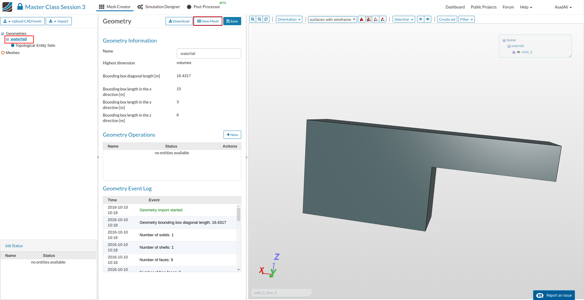
For this project we will use a simple geometry which can be imported using this link.
-
We will examine the waterfall in an open channel with the water entering from one side of the domain and falling into the water reservoir at the bottom of the domain.
Meshing
- Make sure that the geometry item is selected in the Project Tree and press New Mesh to create a new mesh setup for the geometry.
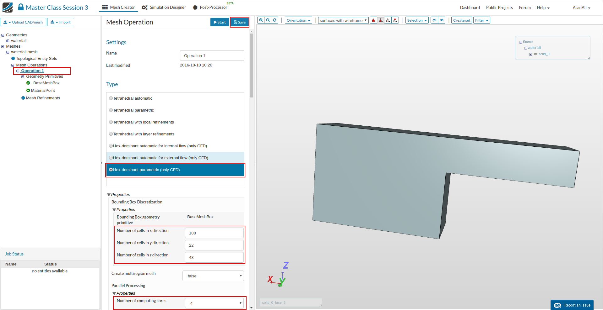
- We will make a fine mesh for this geometry by using the manual Hex-Dominant meshing algorithm. Move to the Hex-dominant parametric (only CFD) in the mesh setup, set the number of cells in the x,y,z directions to 108, 22, and 43 respectively and set the number of cores to 4 for this job.
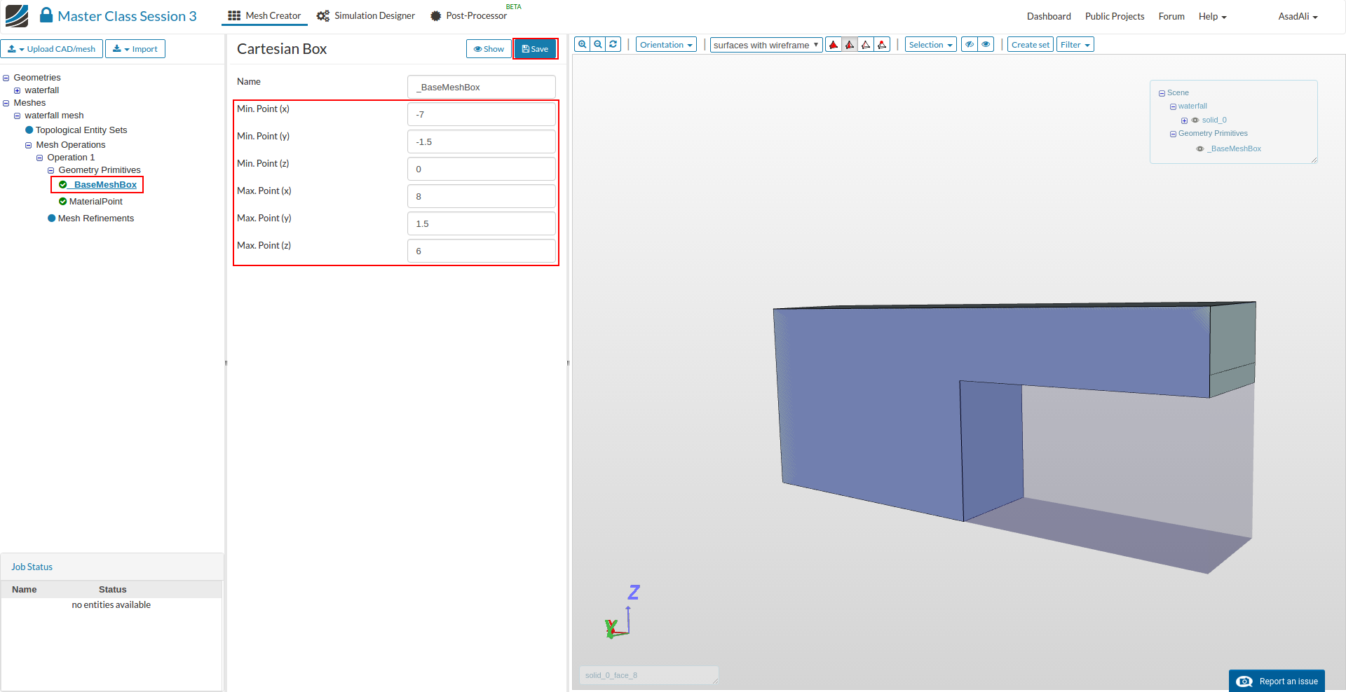
- Now move to the _BaseMeshBox in the mesh tree and set the dimensions for the bounding box as shown in the image below.
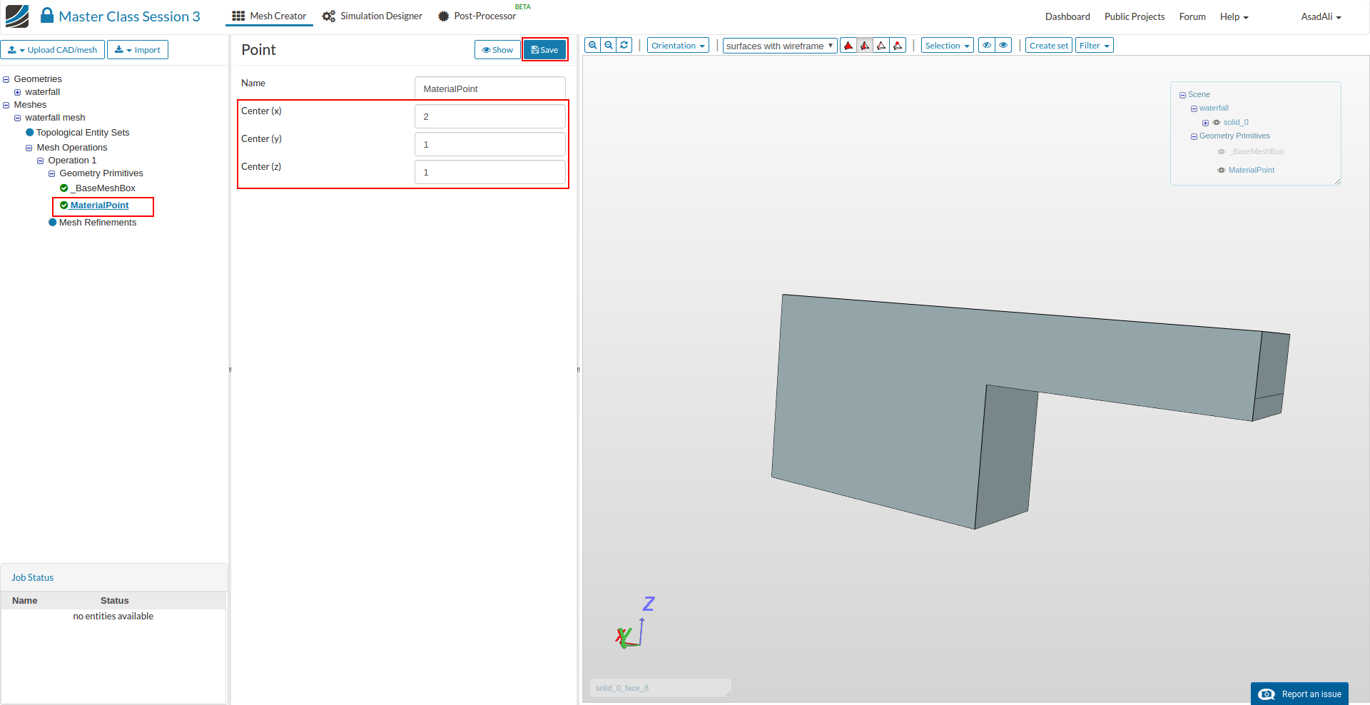
- Next go to the MaterialPoint item in the Project Tree and set the coordinates to (2,1,1).
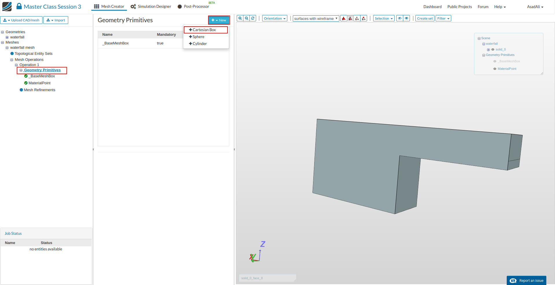
- We want to make mesh refinements as well. To do this, we will create a Cartesian box. Go to the Geometry Primitives item, press New and select Cartesian Box.
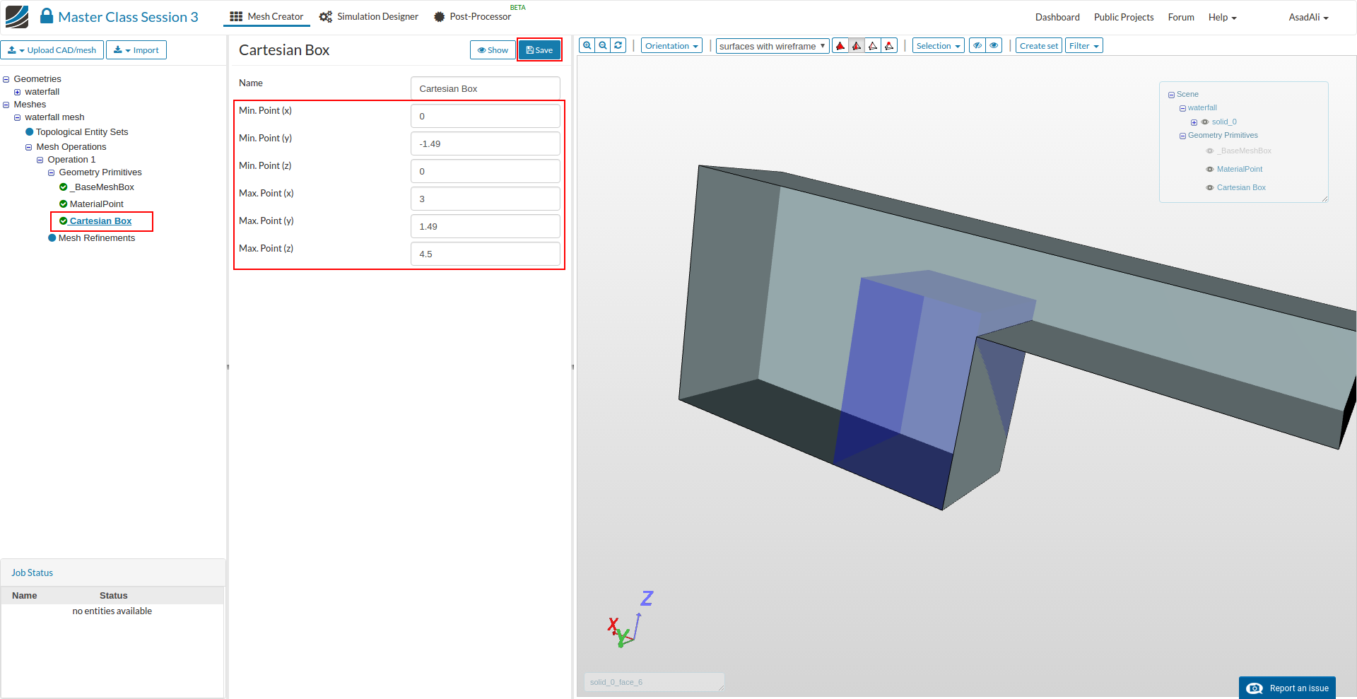
- Set the dimensions of the box as shown in the image below.
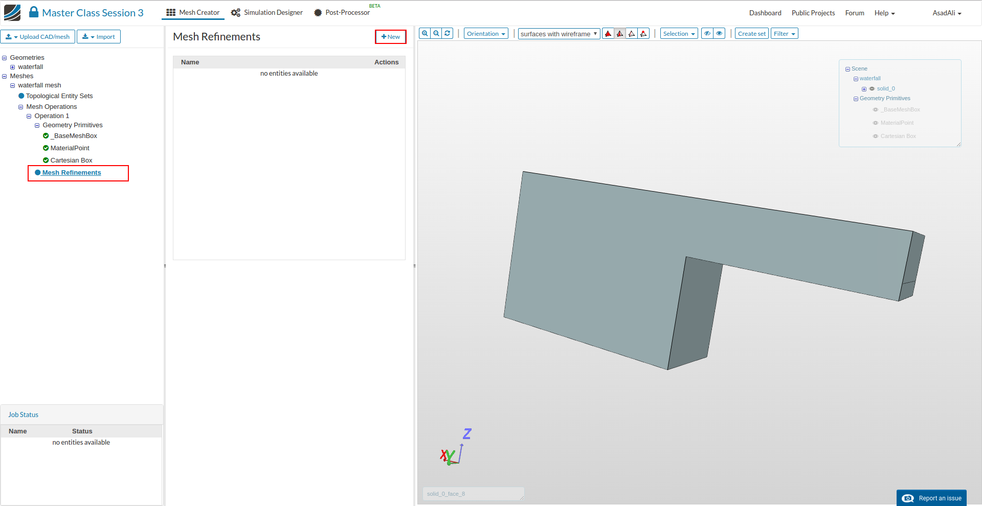
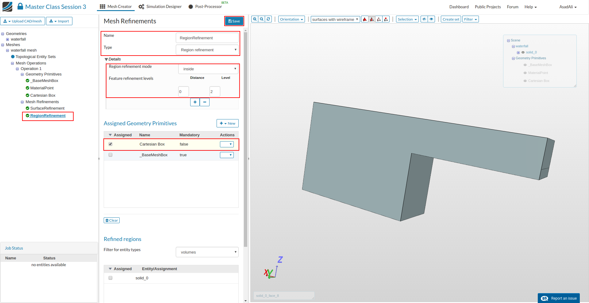
- Now to add mesh refinements, move to the Mesh Refinements in the meshing tree and press New.
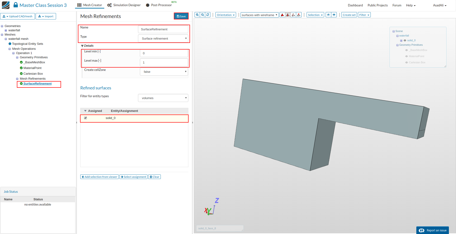
- Rename the mesh refinement to “SurfaceRefinement”, change the refinement type to Surface Refinement, set the refinement levels to 0 and 1, and then Save the selection.
- Similarly add another mesh refinement and name it "RegionRefinement, change the type to Region Refinement. Set the refinement level and assign the refinement to your Cartesian Box geometry primitive. Save the selection.
- Finally move back to Operation 1 in the Project Tree and press Start to start the meshing.
Simulation
- Once the mesh is finished (please note that this can take some time), move to the Simulation Designer tab and press New to start new simulation setup.

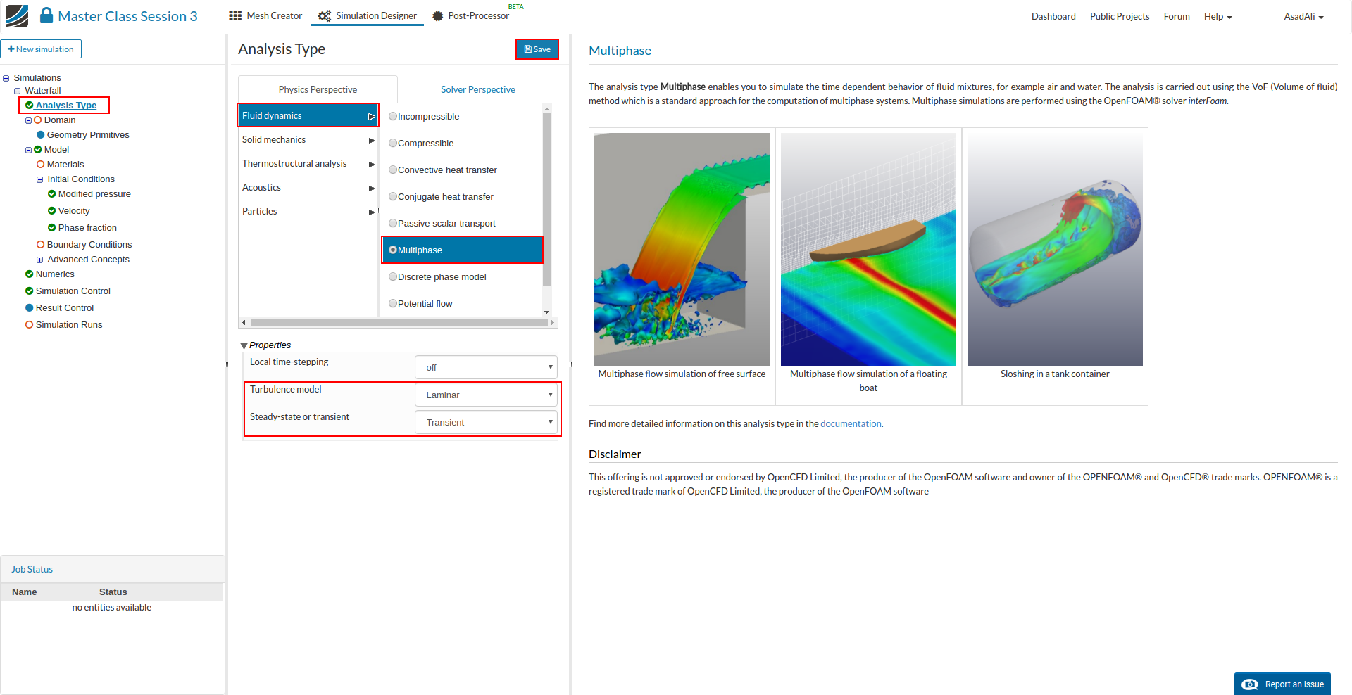
- In the middle column select Fluid dynamics and Multiphase for the Analysis Type. Make sure in the properties that local time stepping is turned off and that the Laminar/Transient model is selected. Once saved the Project Tree will expand in the left column.
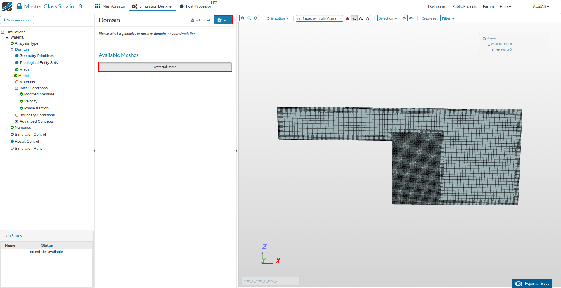
- Go to the Domain item in the Project Tree and assign the mesh. Save the selection. For this simulation we will use the waterfall mesh domain that we just created.
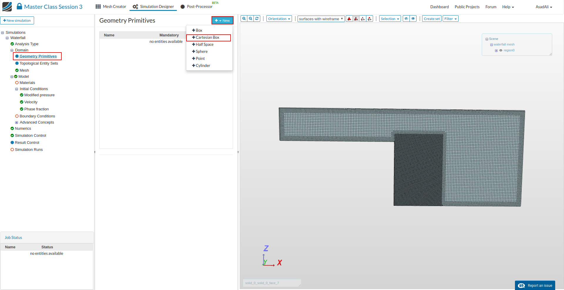
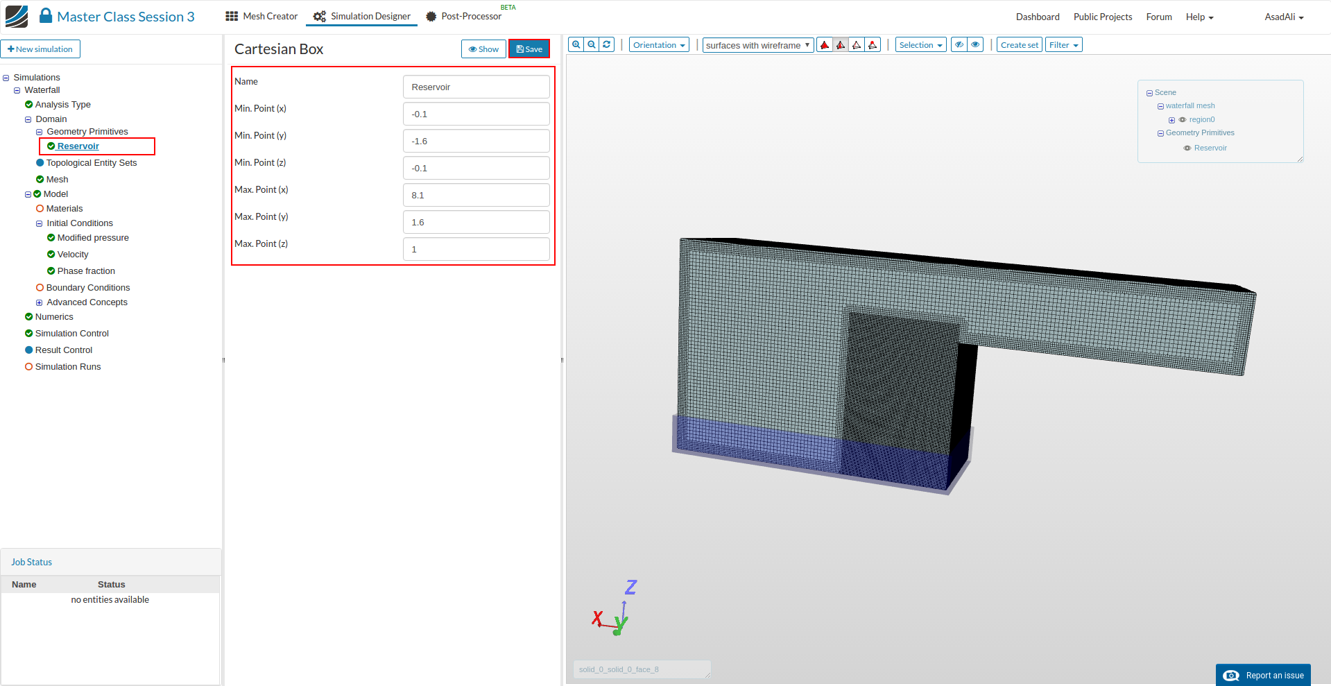
- To create the reservoir of water, move to the Geometry Primitives in the Project Tree and add a new “Cartesian Box”. Rename the box to “Reservoir” and set the dimensions of the box to the values shown in the image below.
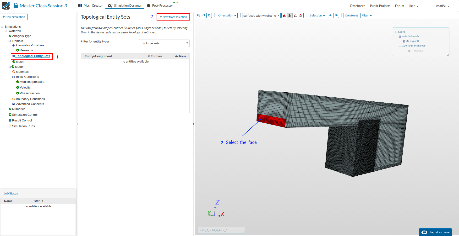
- Now move to the item called Topological Entity Sets, select the inlet face as shown in the image and press +New from selection. Rename this selection to ''inlet".
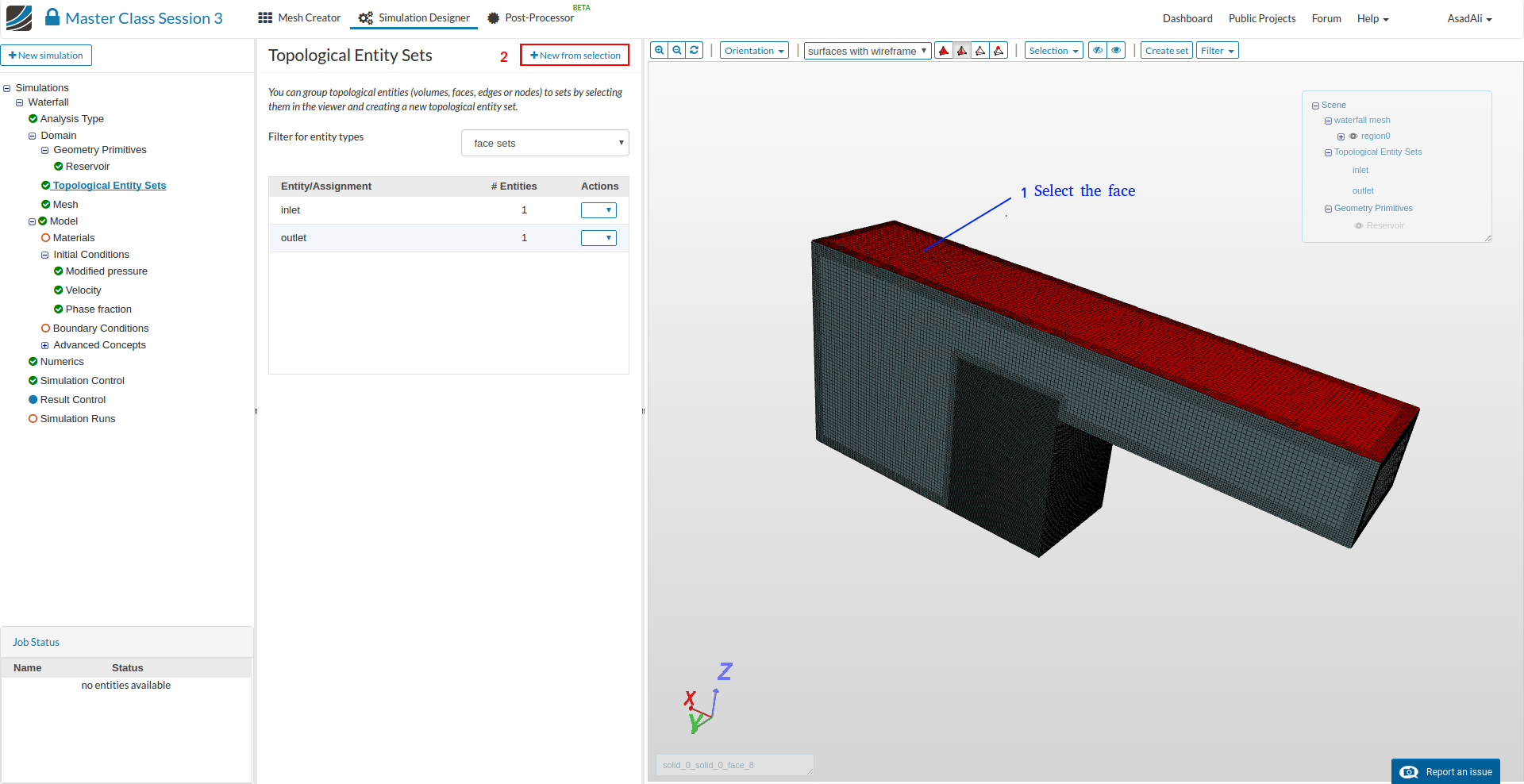
- Similarly select the outlet face as shown in the image below and make a new set. Rename it to “outlet”.
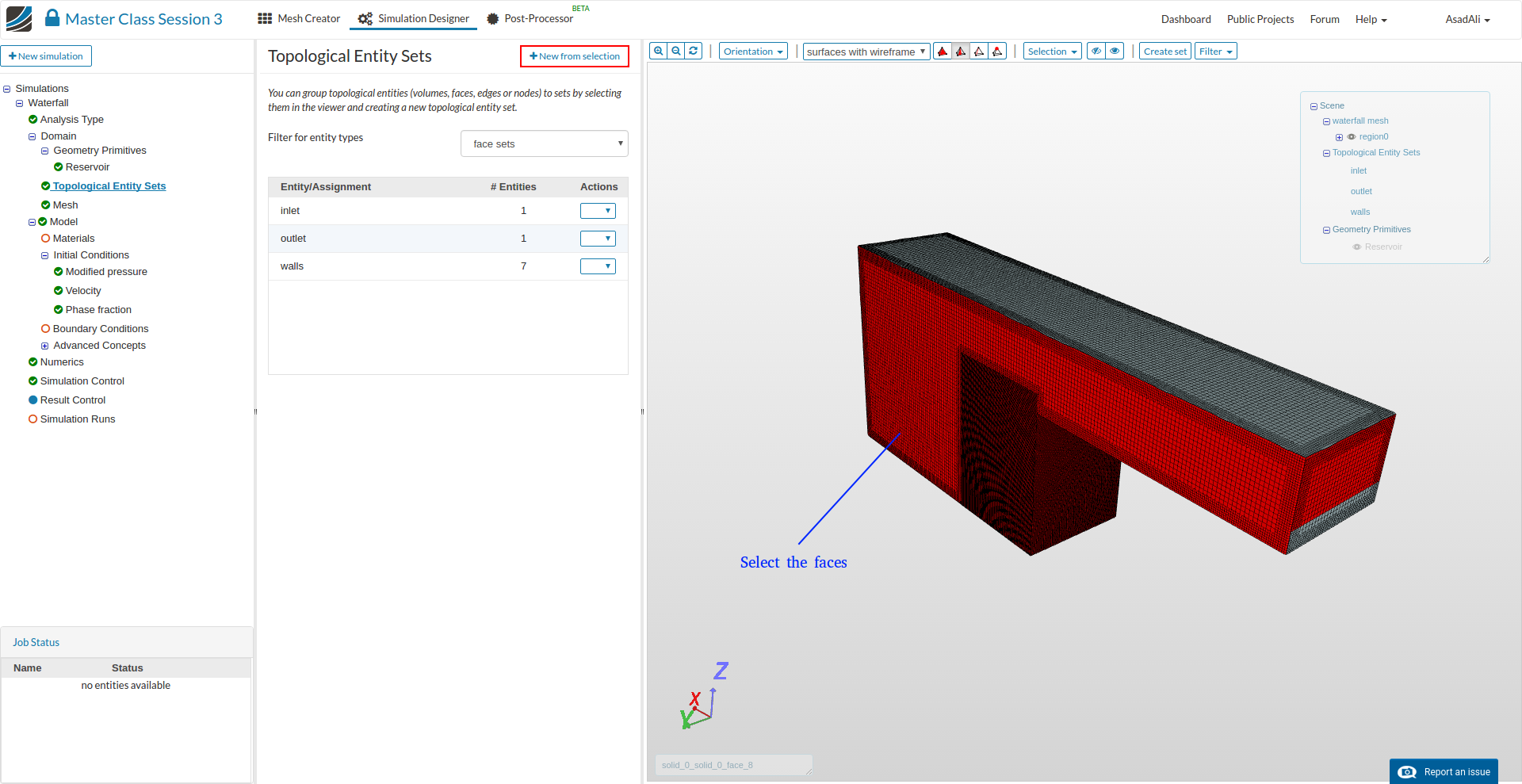
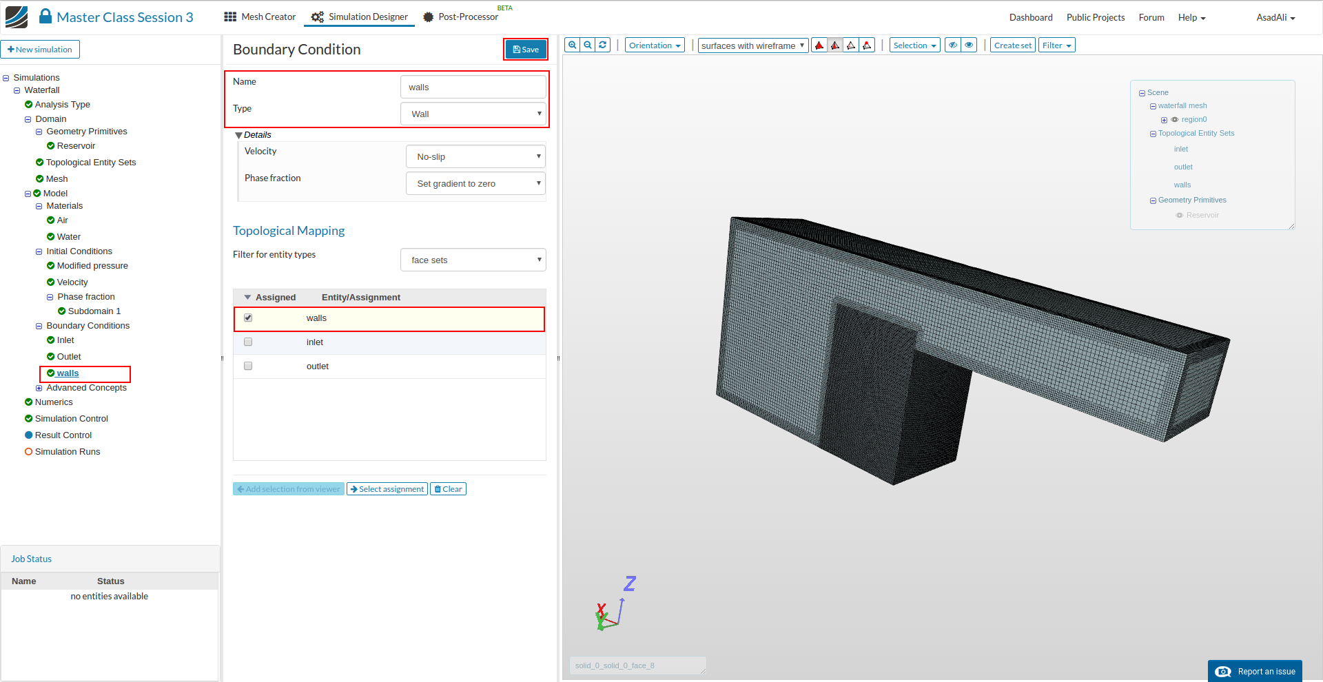
- Finally select the remaining faces and make a new set called “walls”.
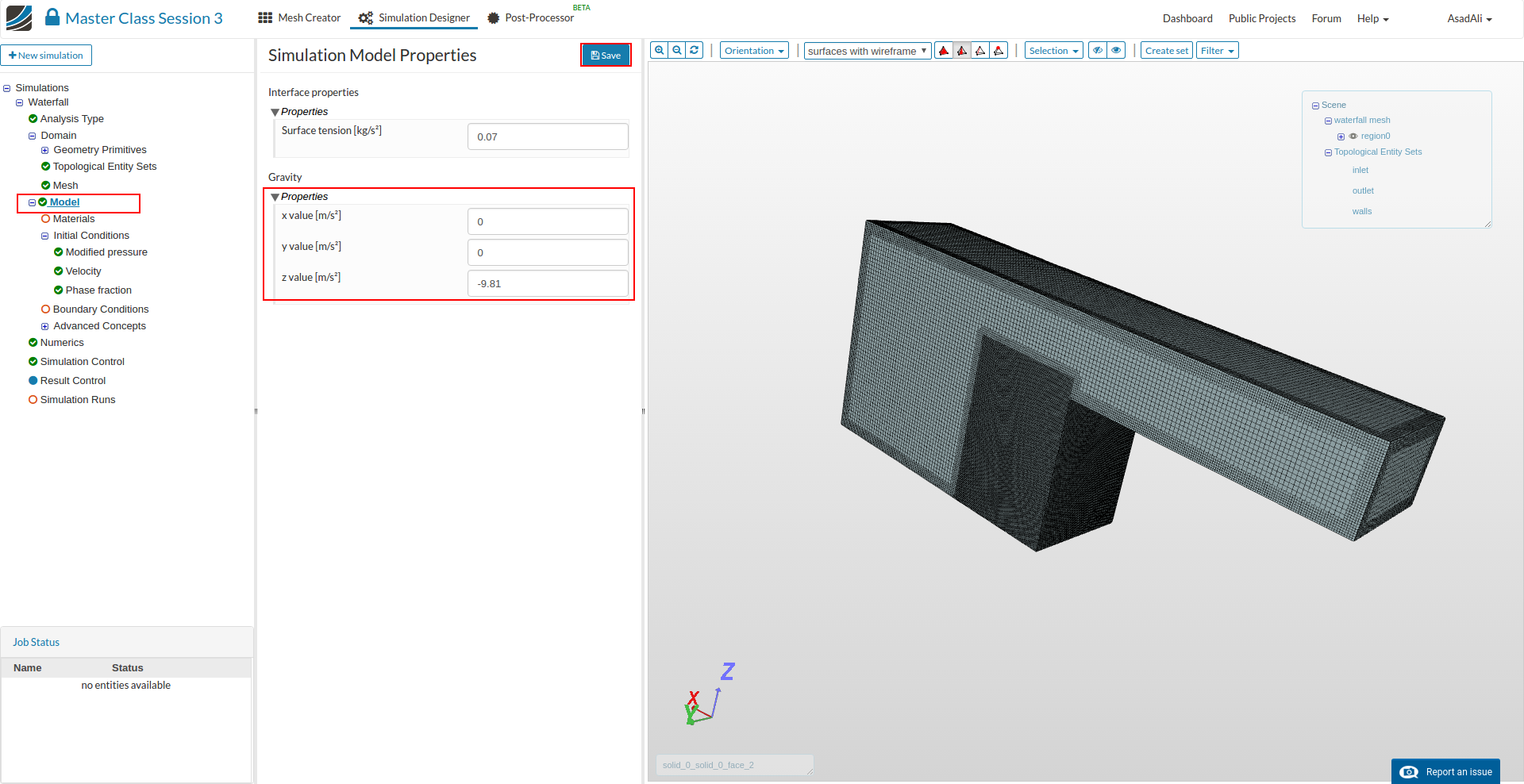
- Now move to the Model item in the Project Tree and set the value for gravity to =9.81 m/s2 for the z value.
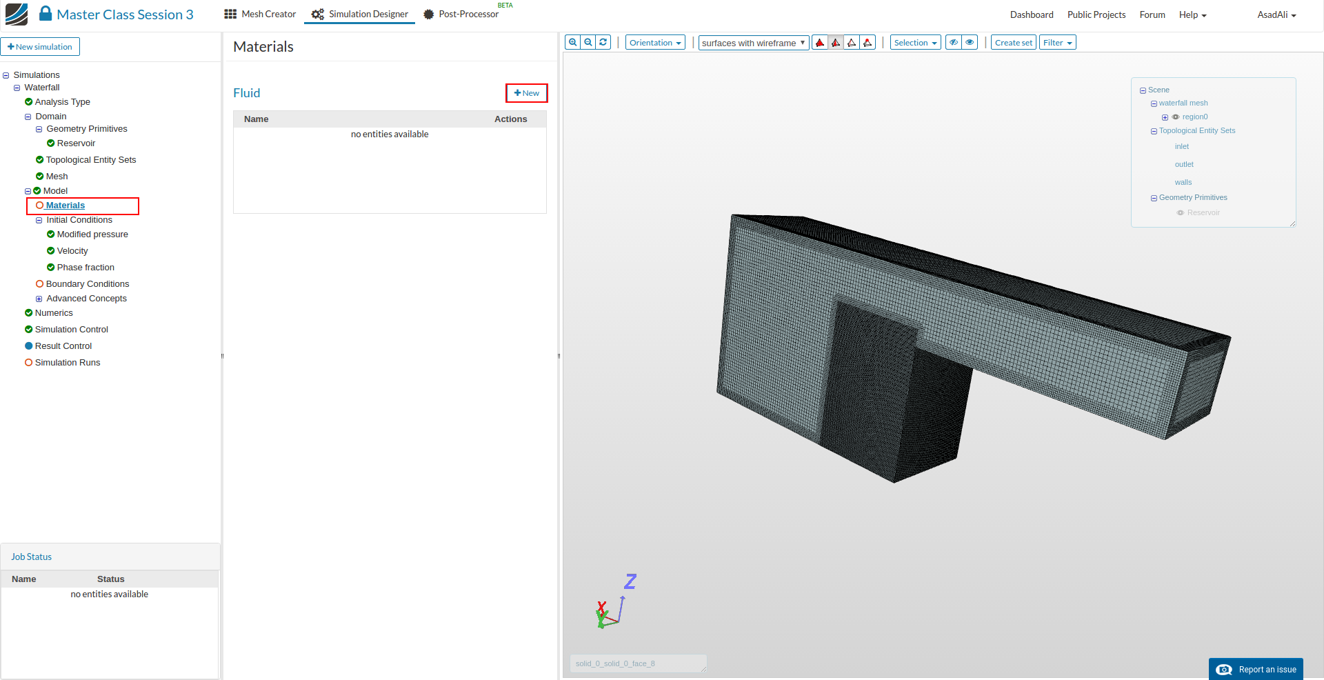
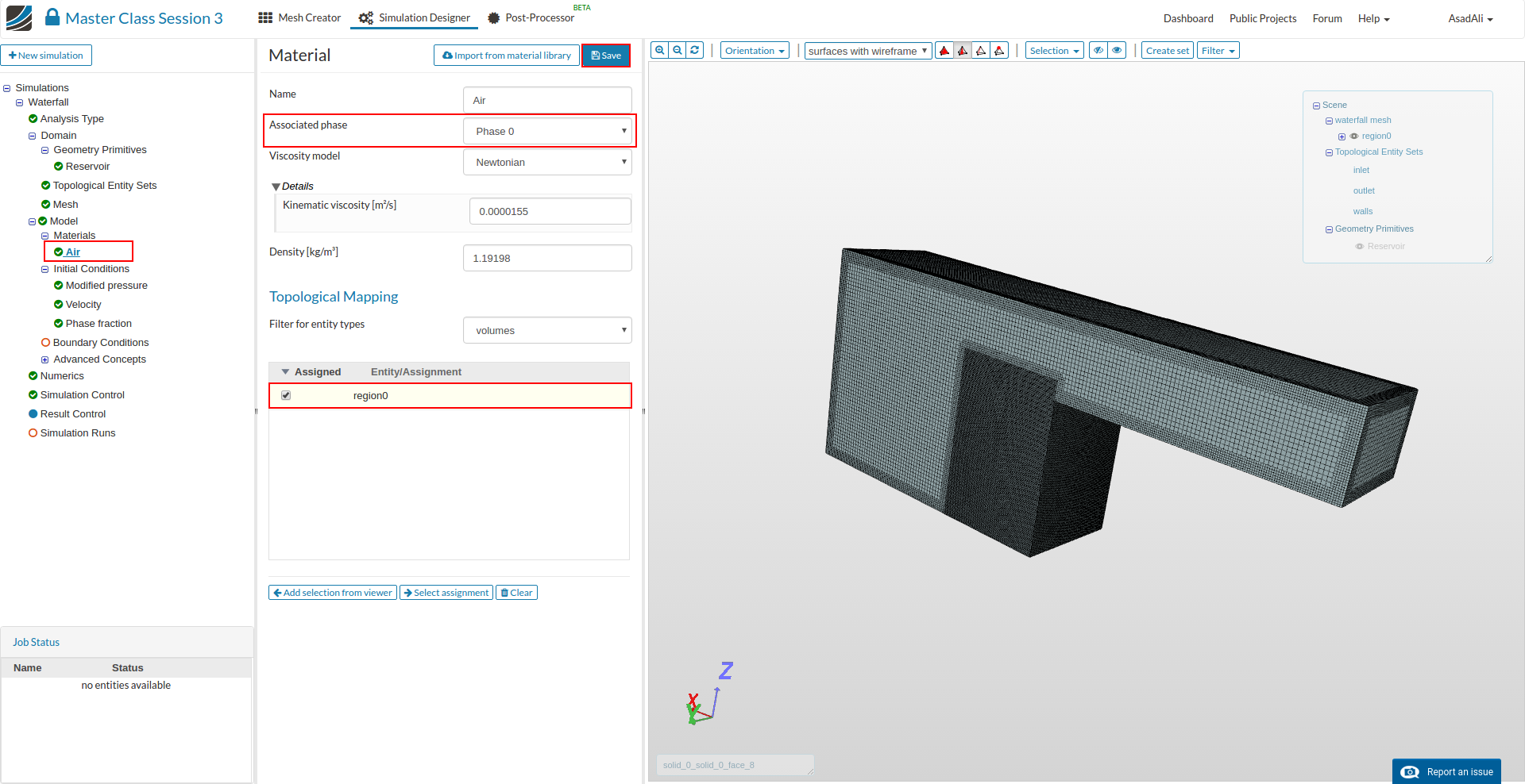
- To assign materials to the domain, move to the Materials and click New.
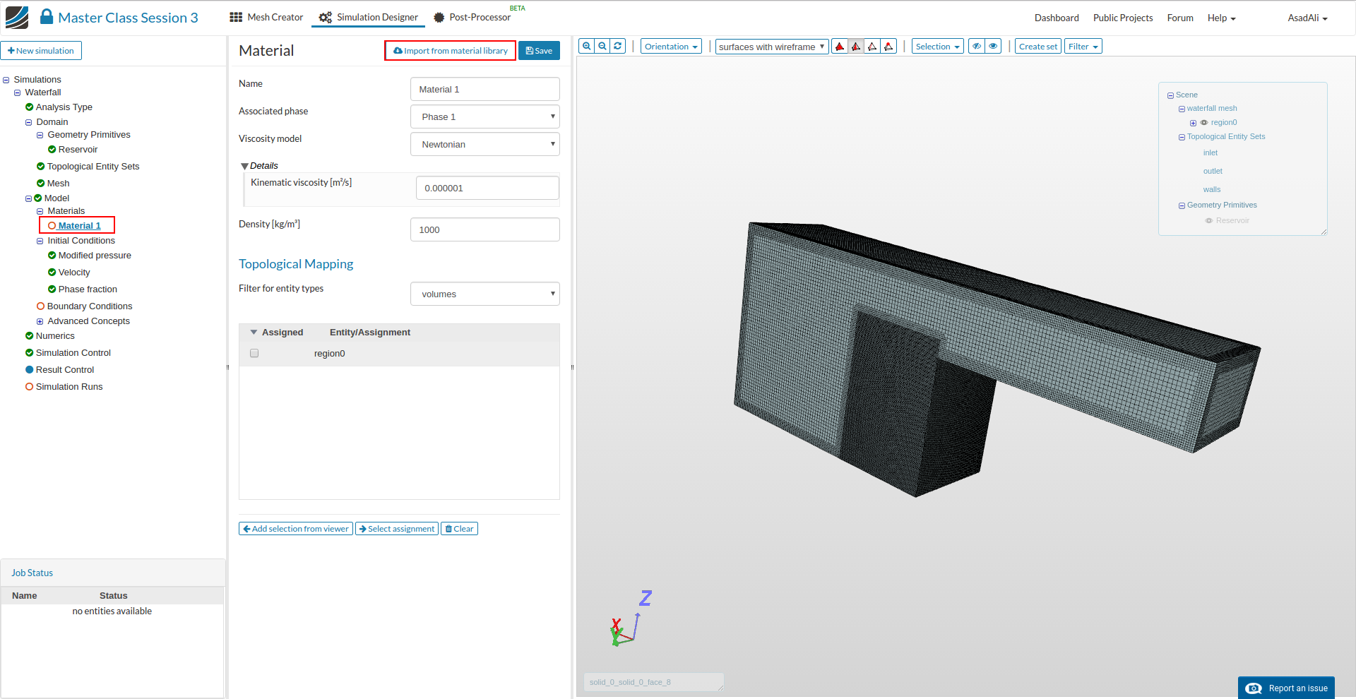
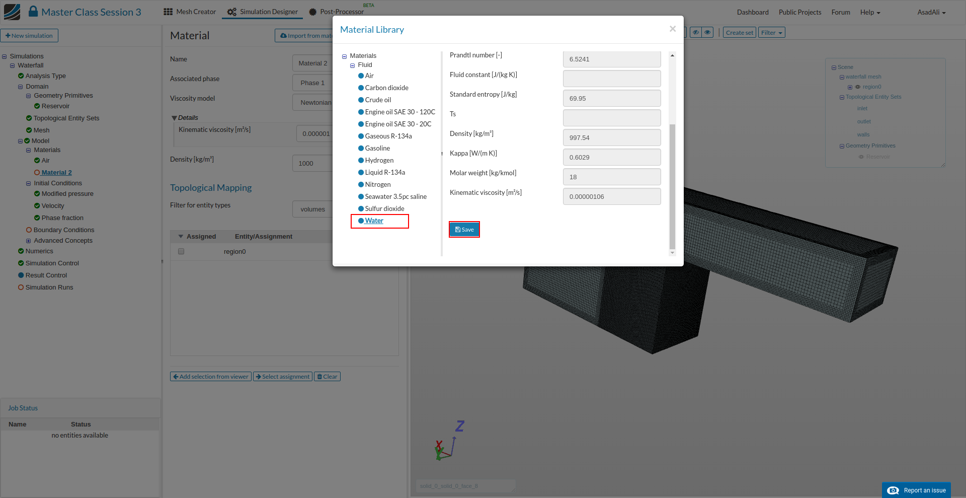
- Click Import from material library.
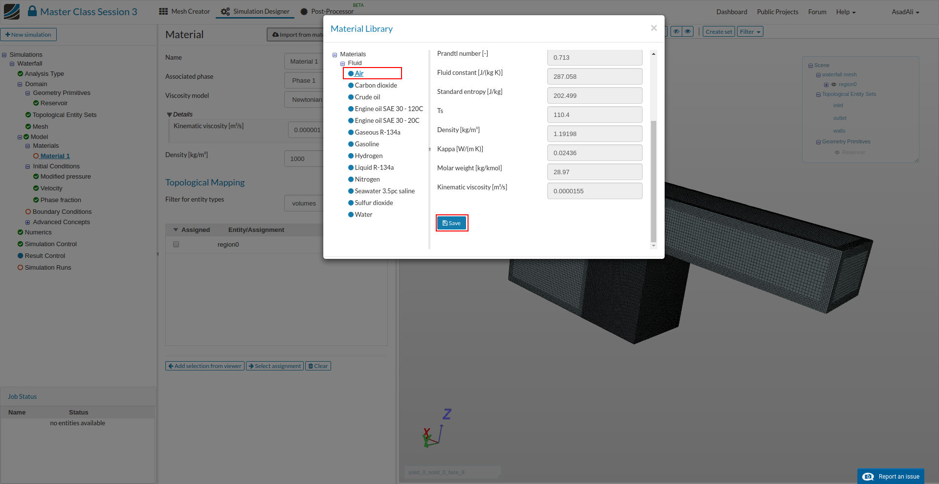
- From the library options, select and save Air.
- Finally change the Associated phase to “Phase 0” and assign it to the entire volume region0
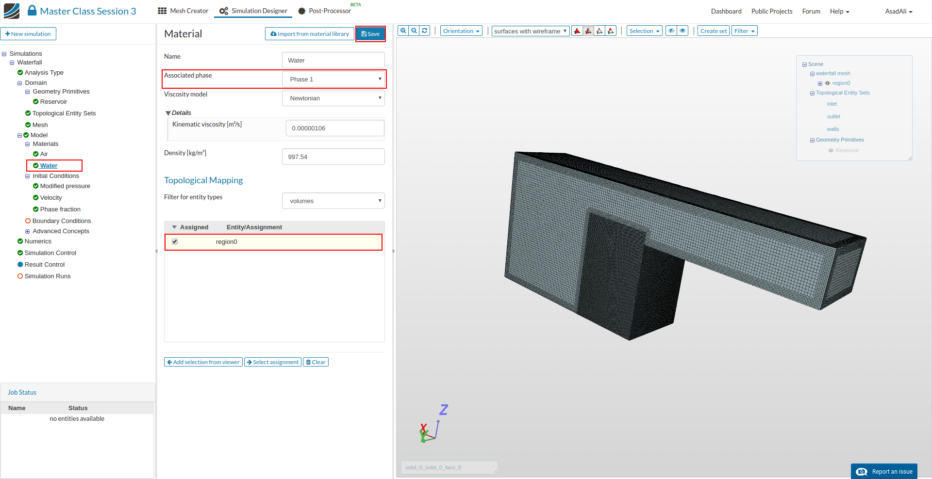
- Similarly add another material, this time Water.
- Change the Associated phase to “Phase 1” and assign it to the entire volume region0
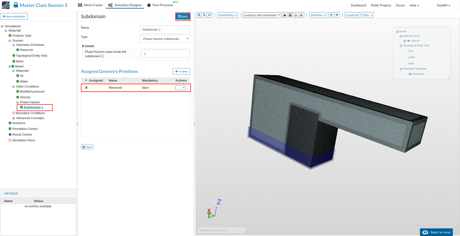
- Now move to the Phase fraction in initial conditions, change the type to Subdomain-based and set the “Default phase fraction value” to 0. Press Save to save the selection.
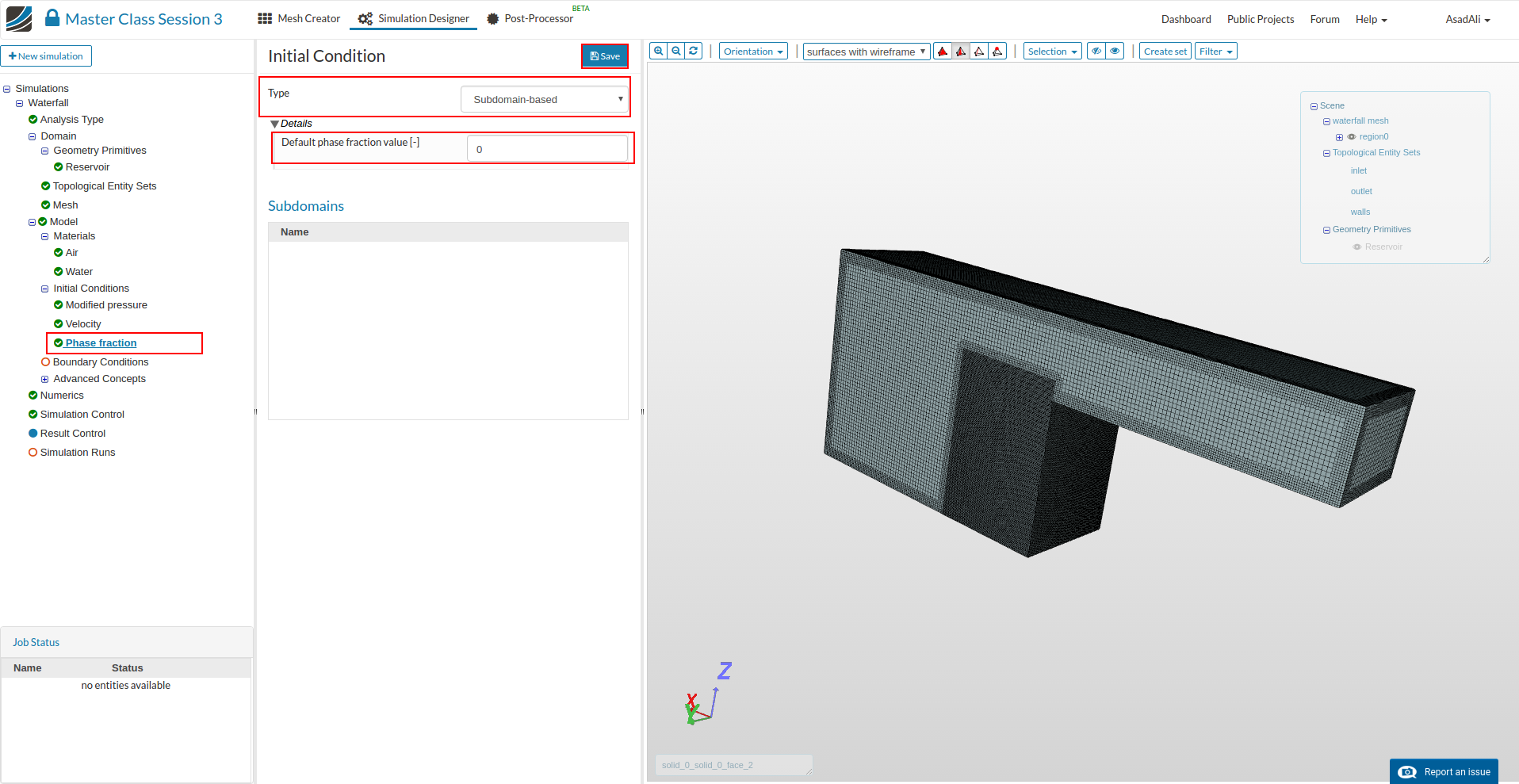
- Once saved, press New to add the subdomain. Here set the parameters accordingly, select the “Reservoir” and save the selection.
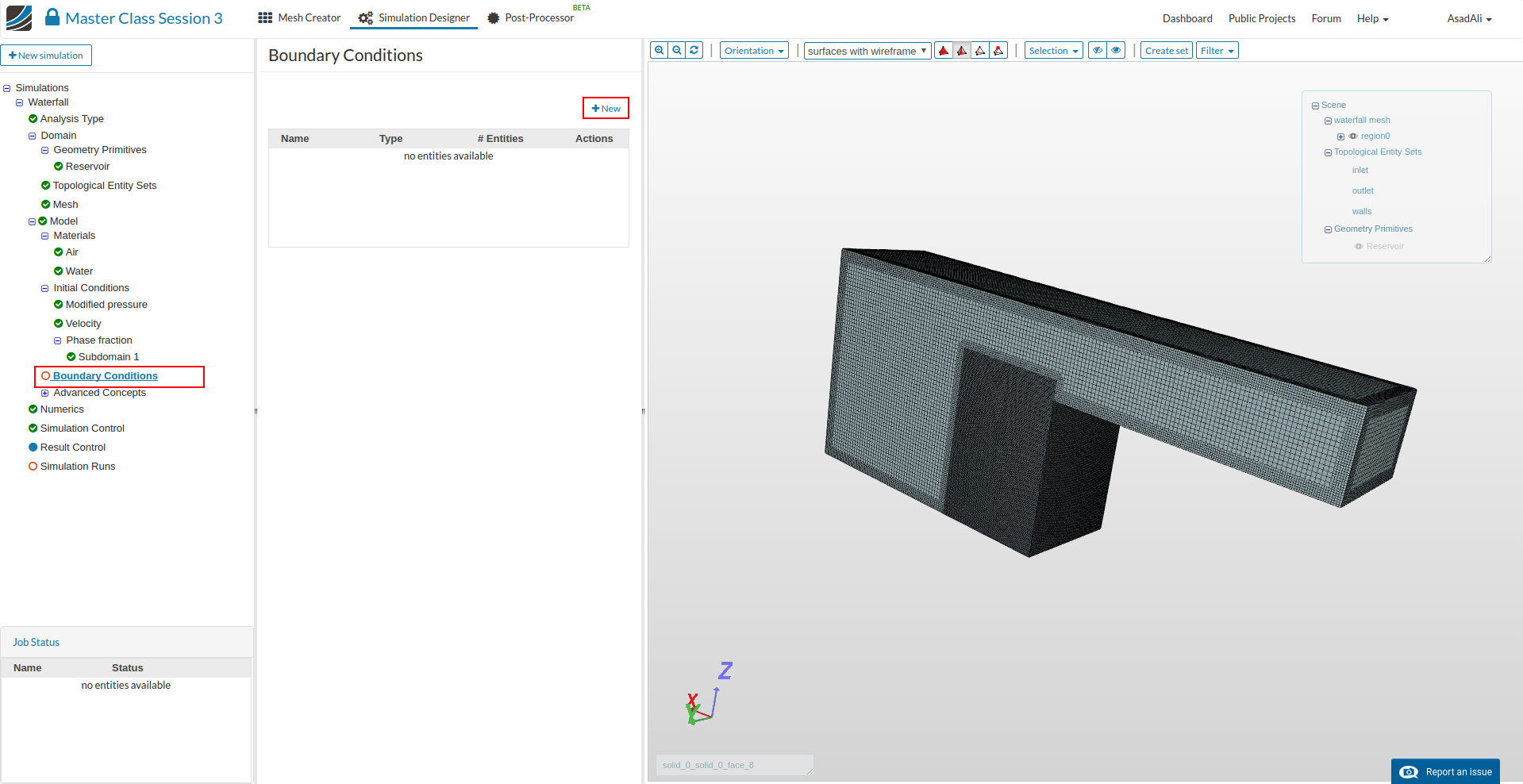
- The next step is to add the boundary conditions. Move to the Boundary conditions item in the Project Tree and press New to add a new boundary condition.
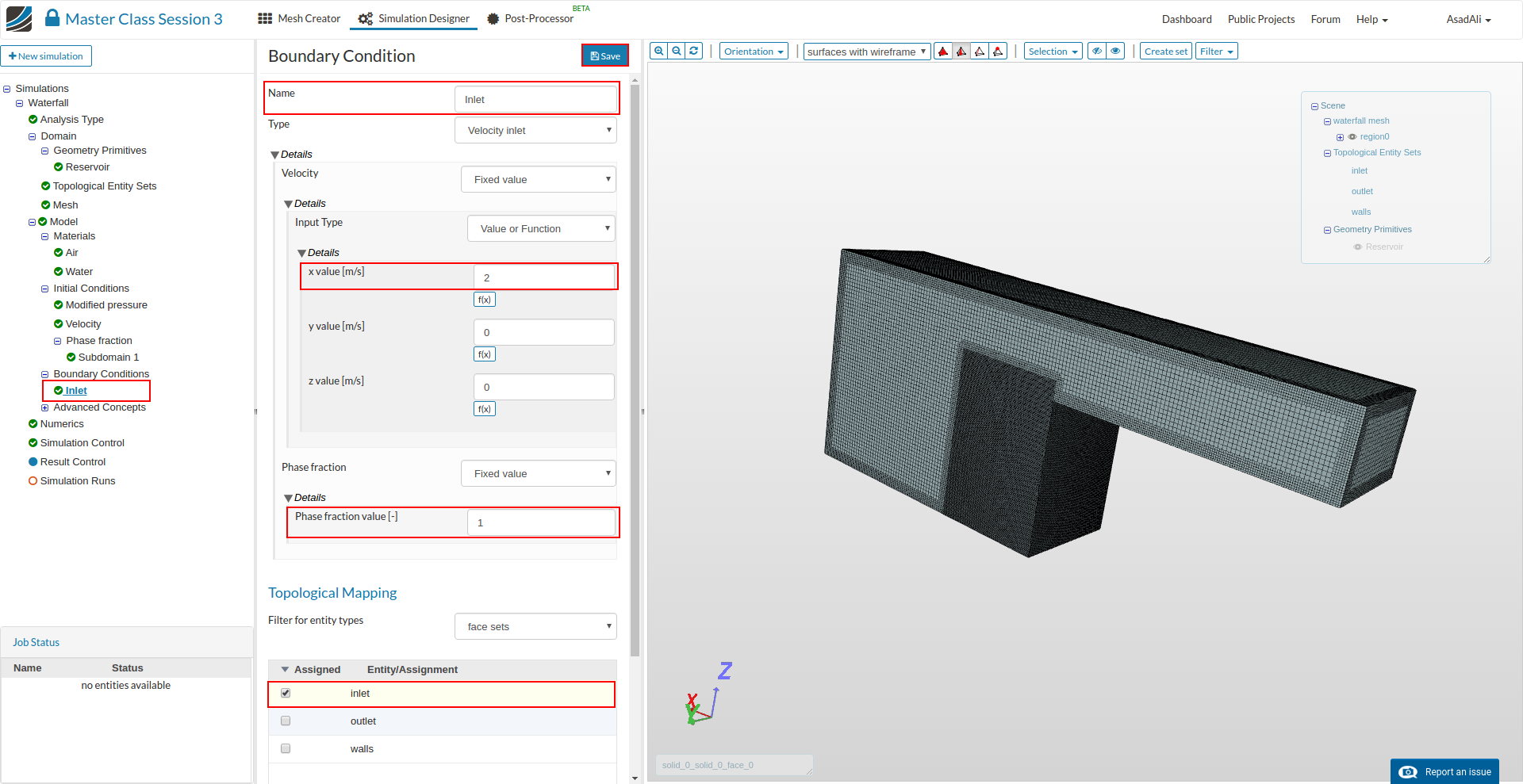
- Rename the boundary condition to “Inlet”, set the Type to Velocity Inlet with an x value velocity of 2 m/s, set the phase fraction to 1 and assign it to the “inlet” face. Press Save to save the selection.
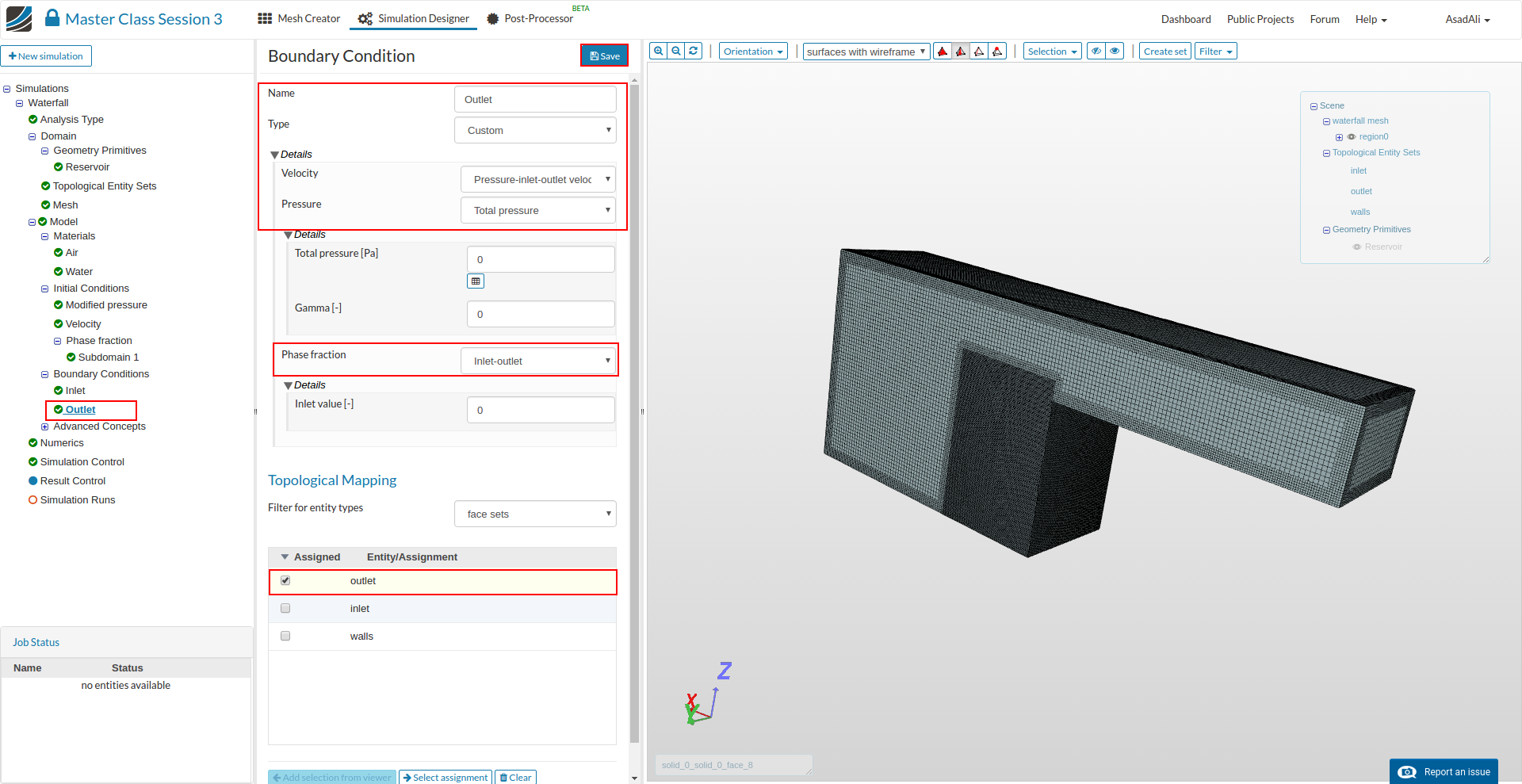
- Add another boundary condition for the outlet and rename it to “Outlet”. Set the Type to Custom with a pressure-inlet outlet velocity and Total pressure. Then set the phase fraction to Inlet-outlet and assign it to the “outlet” face. Press Save to save the selection.
- Add the last boundary condition for the walls as shown in the image.
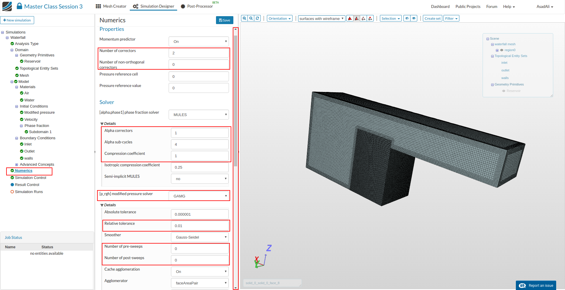
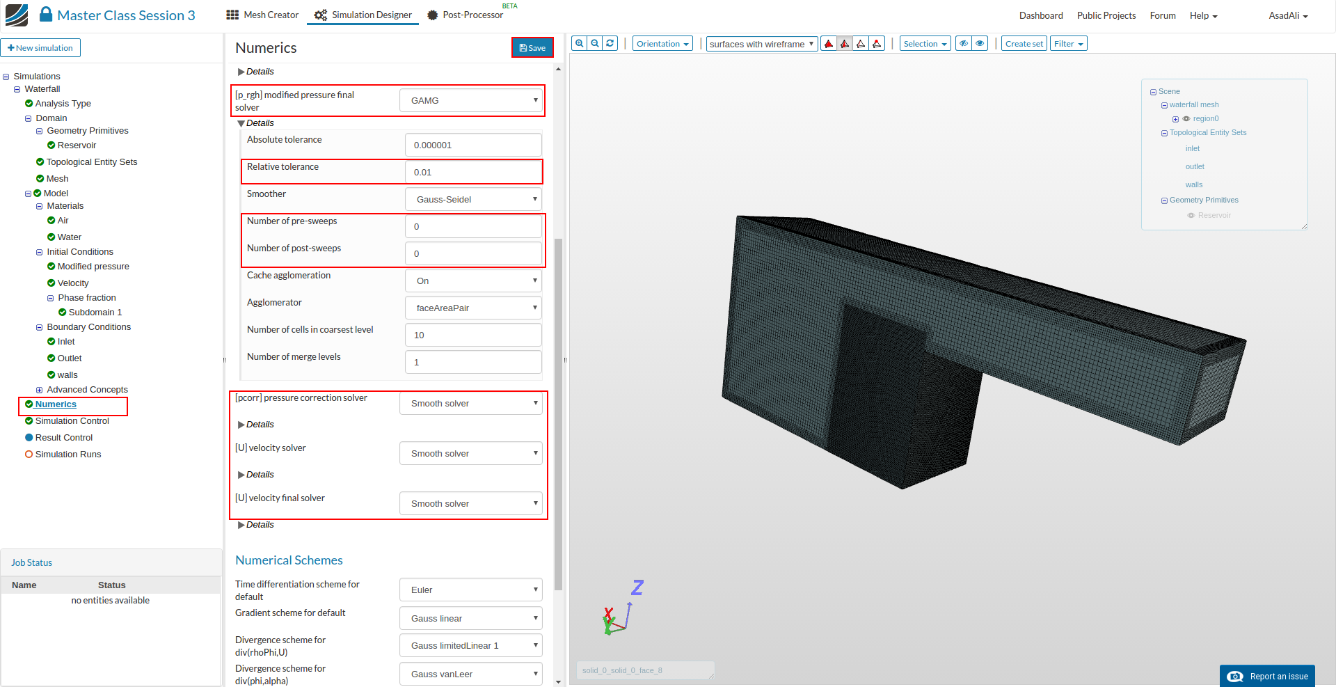
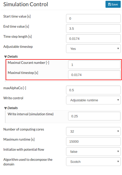
- Now move to the Numerics and set the essential parameters as shown in the images below. Press Save to save the selection.
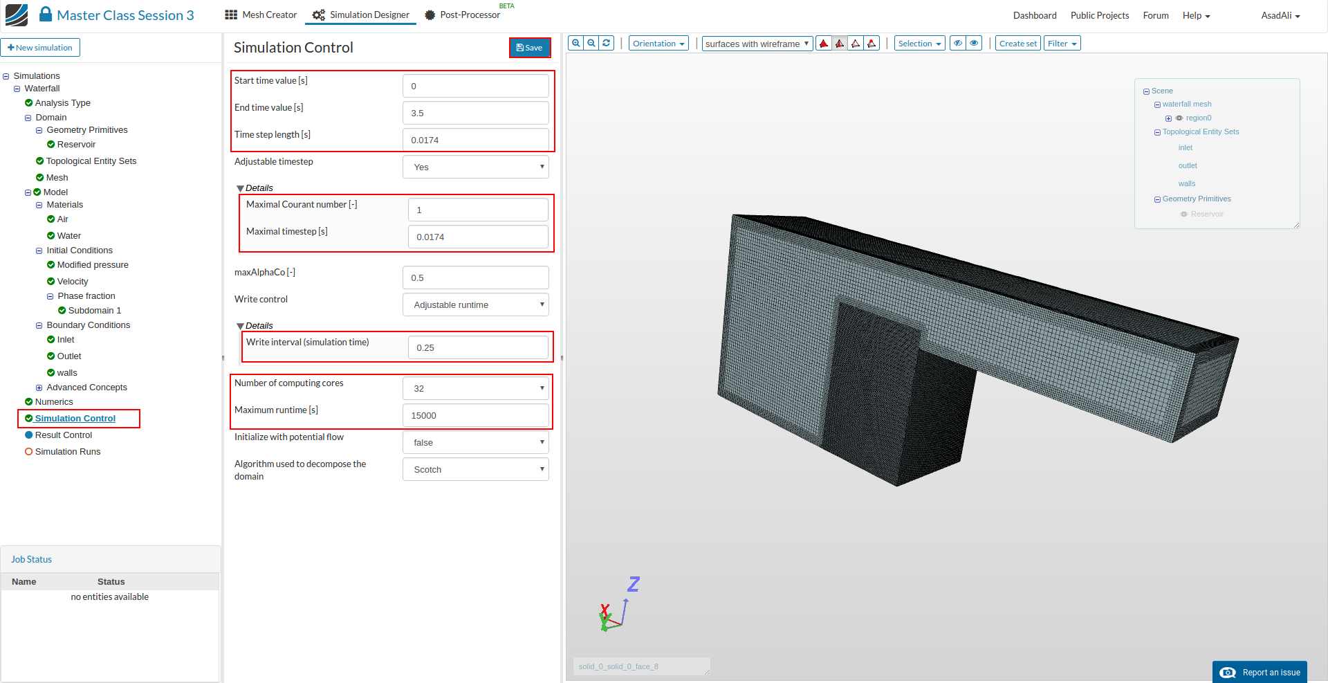
- Move to the Simulation control and set the parameters accordingly. We will run this simulation for 3.5 seconds. Save the selection.
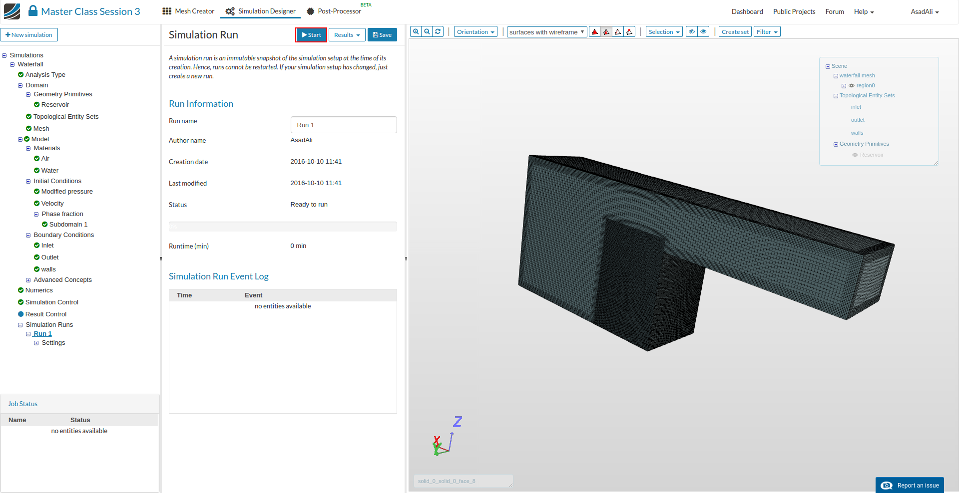
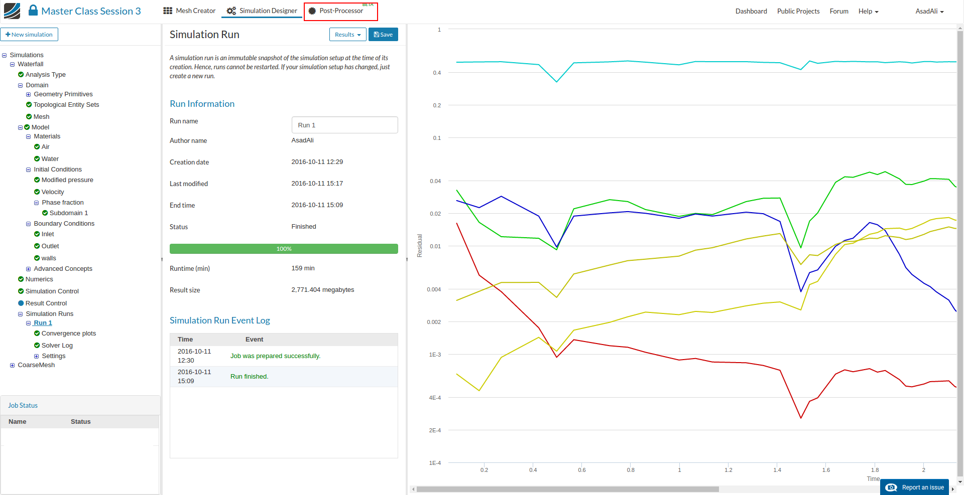
- Then move to the Simulation Runs item in the Project Tree and press New to create a new simulation run. Once new run is created press Start to start the simulation run.
Post-processing
- Once the simulation is complete, move to the Post-Processor tab.
- Load the solution fields to the viewer by clicking on the Solution fields item in the project tree.
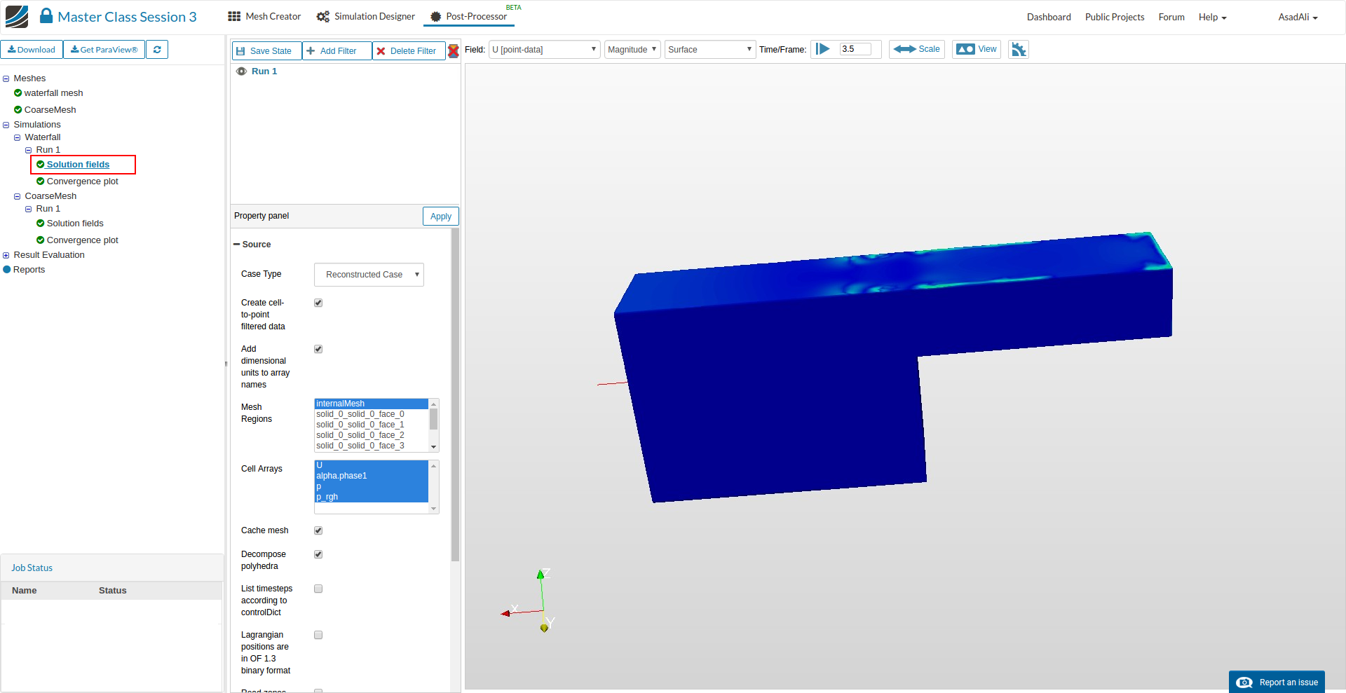
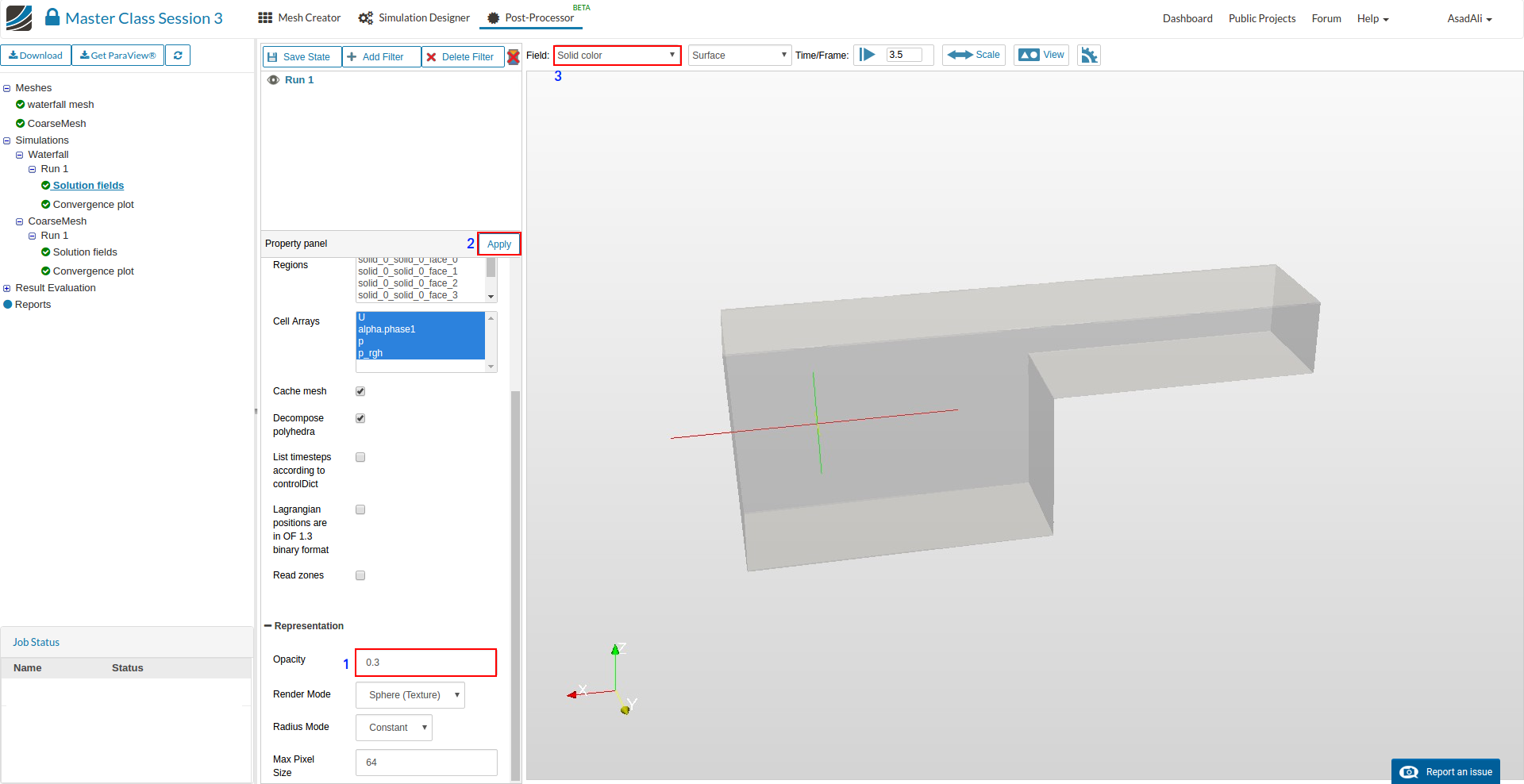
- Once solution is loaded change the Opacity of the domain and Apply the changes. Now change the shown field to Solid color. This way we are only plotting the domain.
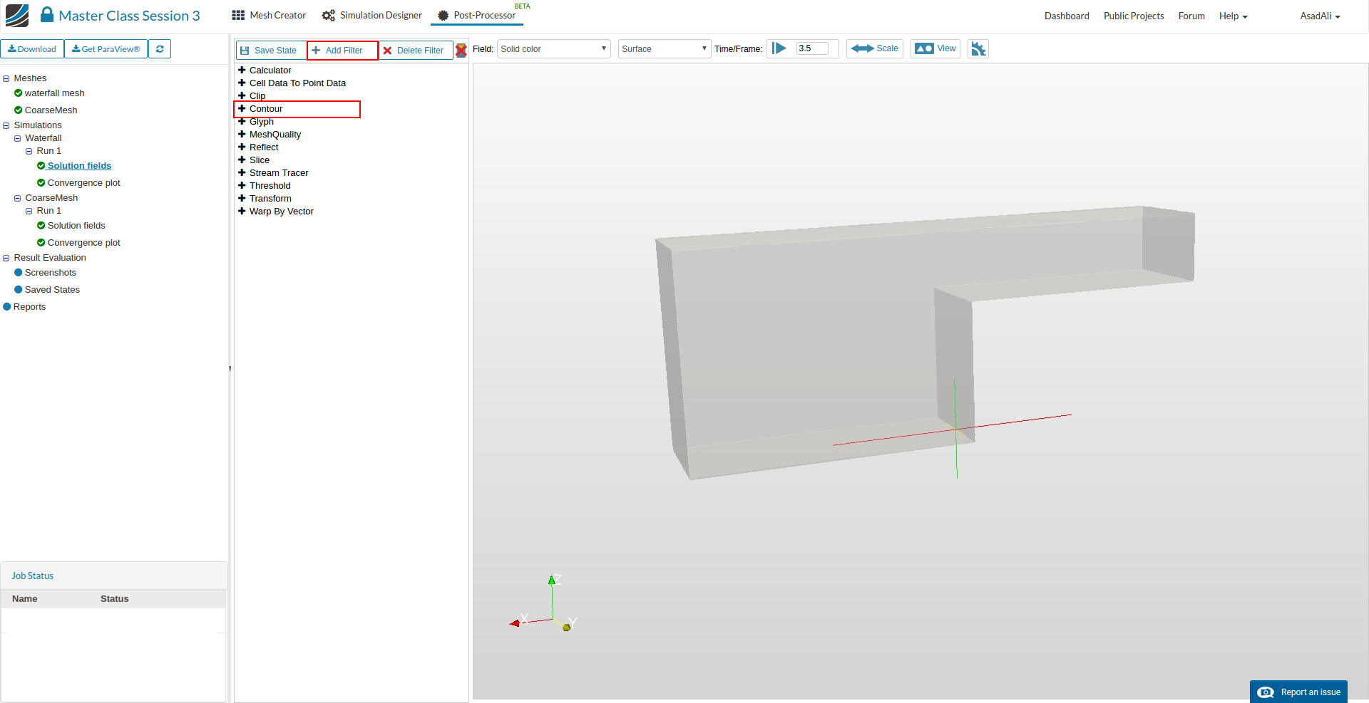
- Next add a filter to visualize the air water interface. Click on the Add filter button and select Contour.
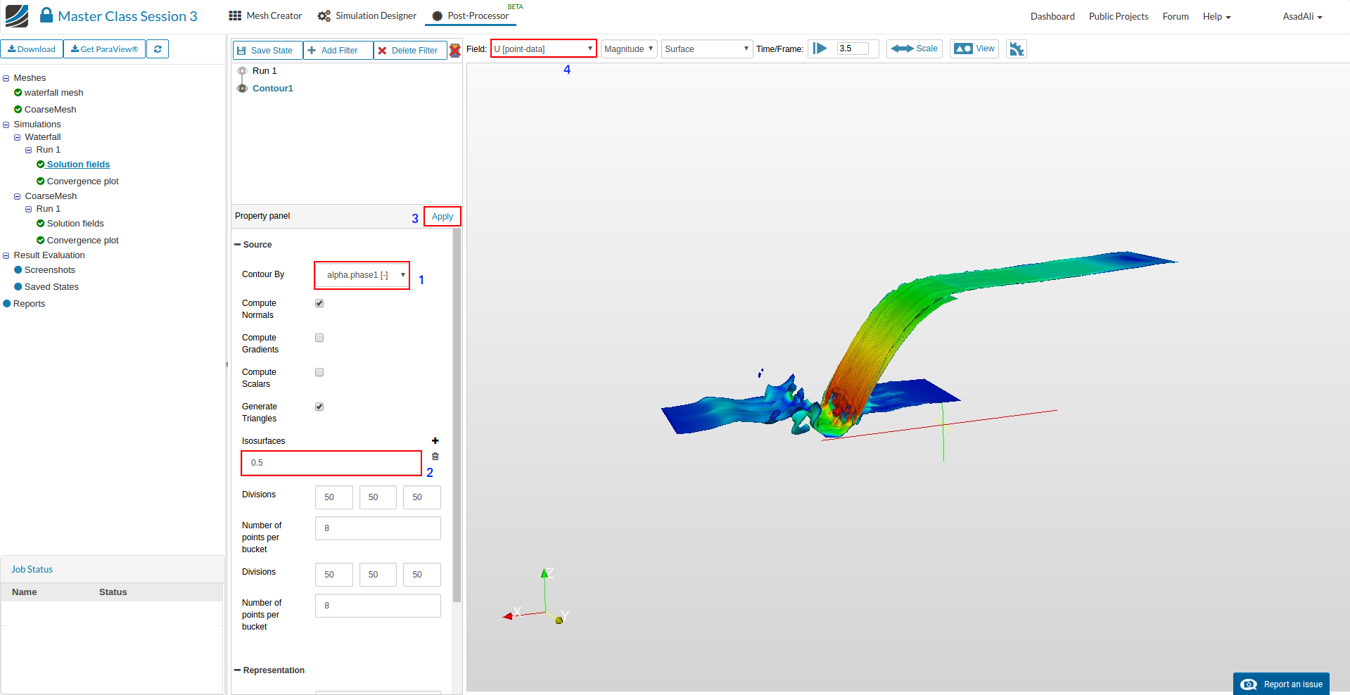
- Set the parameters as shown in the image. Apply the changes and change the plotted field to U in order to visualize the velocity at interface.
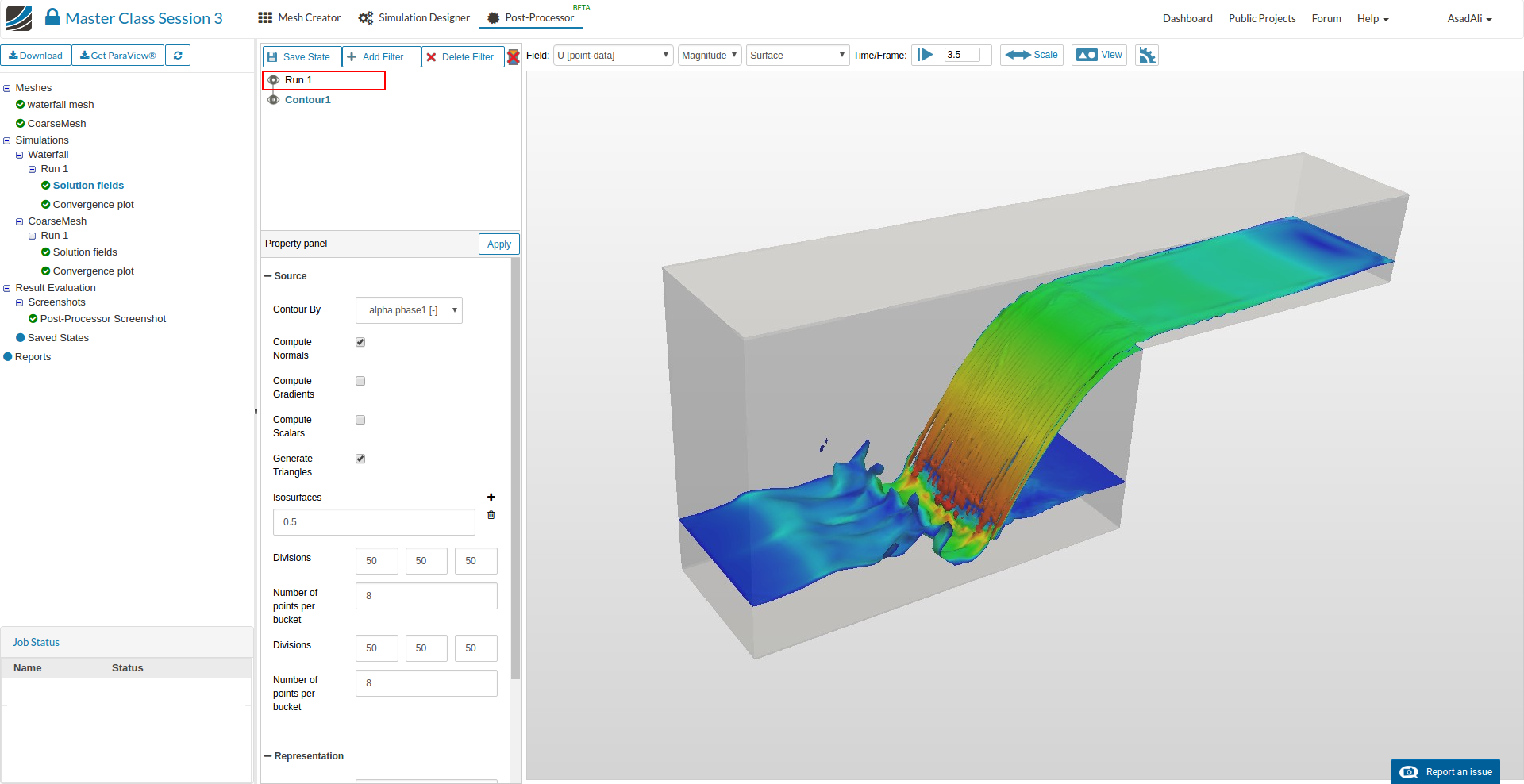
- Click on the eye sign next to the “Run 1” item to show the domain.
-
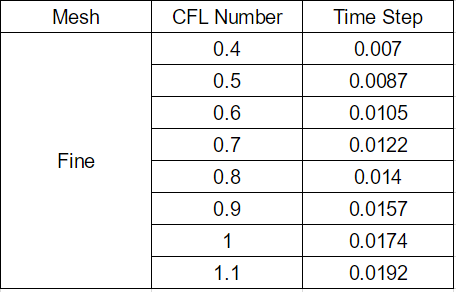
Now your task is to examine how changing the Courant numbers and time step affects the convergence speed and stability of the simulation. Create a table to track your findings.
-
Please create additional simulation runs for following time steps/Courant numbers:
 But creating a plot showing the execution time over CFL for instance would be a nice “add-on” inside the homework documentation indeed.