Step-by-Step Tutorial: Dynamic Drop Test of a Skateboard with SimScale Add-in for Fusion 360

nava · August 16, 2016, 8:53am

Recording

(will be available soon)

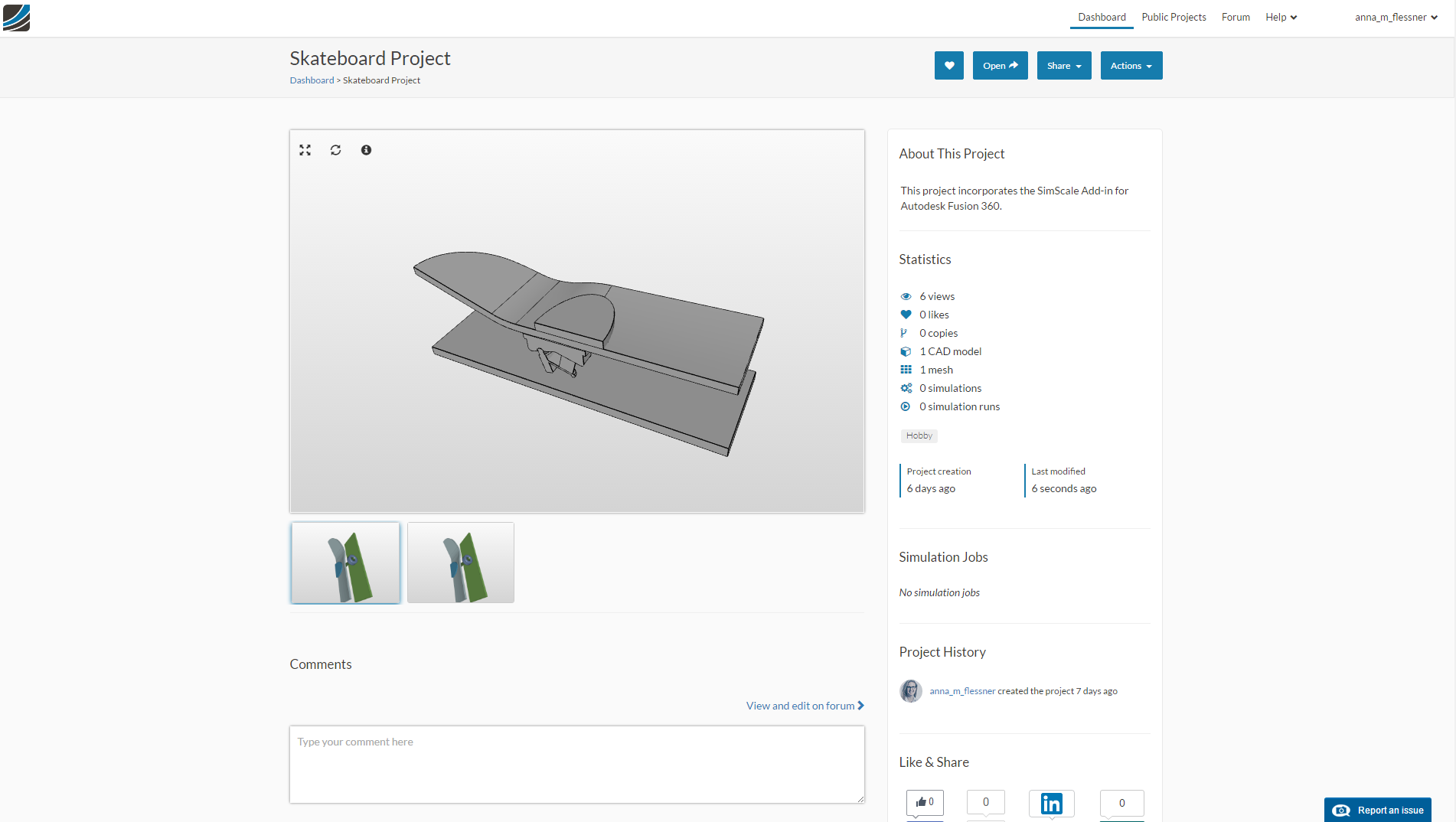
Skateboard Exercise

This exercise tests the durability of a skateboard when it lands on the ground. This involves simulating the stresses on skateboard with a certain initial velocity and a physical contact defined between the wheels and ground. Interesting thing to observe here is the evolution of maximum stress in the skateboard with time.

The weight of the rider is assumed to be 65 kg which is equally distributed between two rubber paddings and therefore, the density of the rubber is calculated by weight on each rubber padding (32.5 kg) divided by its volume (9.3 x 10^-5 m³), which comes out to be 349462 kg/m³. The skateboard is given an initial velocity of 2 m/s as shown in the figure.

Step-by-Step

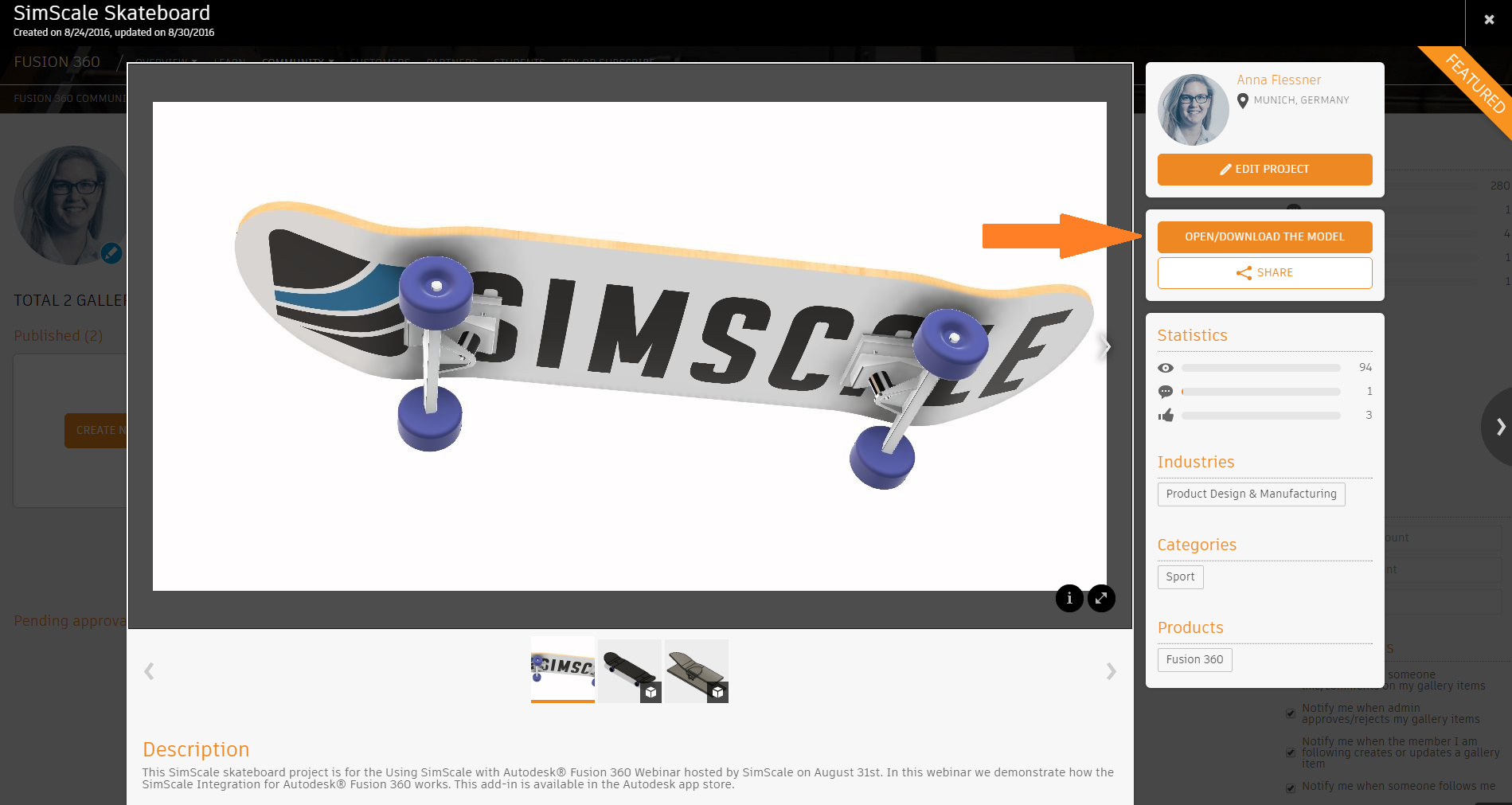
The CAD model of the Skateboard is available in the Fusion 360 Gallery (Link)

Click on the button OPEN/DOWNLOAD THE MODEL in the viewer and then open the Simulation Model in Fusion 360.
To pull the model into SimScale, you will first need to install the SimScale Integration for Autodesk® Fusion 360™ which is now available in the Autodesk App Store for Windows and Mac:

[SimScale Integration for Autodesk® Fusion 360™]
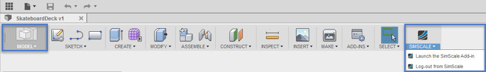
Once the SimScale add-in has been installed you will now see it in the modeling window of Fusion 360

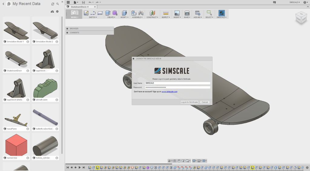
To pull the model into SimScale (Simulation Model 1 in this case), Launch the SimScale Add-in and log in with you SimScale user name or email and password.

After logging in you will be prompted to choose the project from your SimScale Dashboard to which you would like to upload the CAD model. You can create an empty project (no CAD model upload) ahead of time.
If you are new to SimScale, you can sign up for a free account and read this article about how to create a new project

Once the model has been uploaded, you can go to your SimScale Dashboard and see that the CAD model was added to the project that you chose.

Click on OPEN in the upper right hand corner to enter the SimScale workbench where we will set up the simulation as shown in the rest of this tutorial

OR

If you do not have a Fusion 360 Account and would like to start the tutorial, click on the link below to import the Project directly into your workbench.

Directly import the project into my Workbench (Crtl + Click to open in a new tab)

Meshing

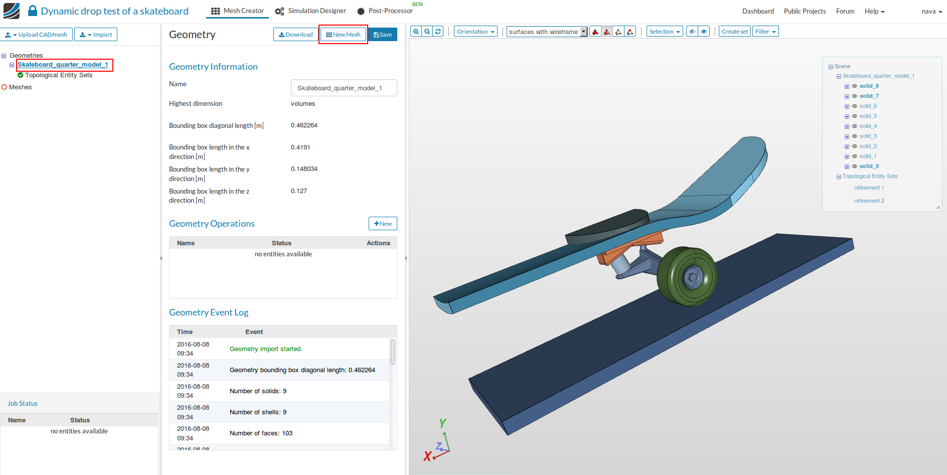
In the ‘Mesh Creator’ tab, click on the geometry ‘Skateboard_quarter_model_1_mesh’
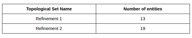
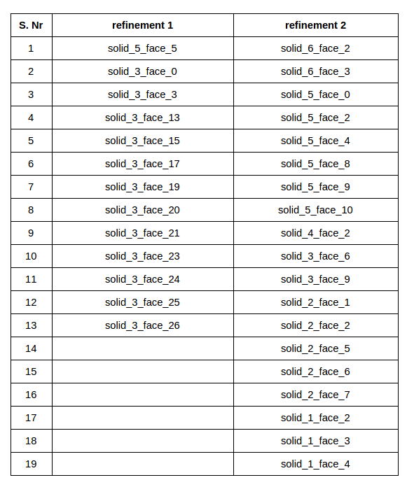
First, we will create two topological entity sets for the mesh refinement as given in the table below.

Go to Topological Entity Sets under Skateboard_quarter_model_1_mesh.
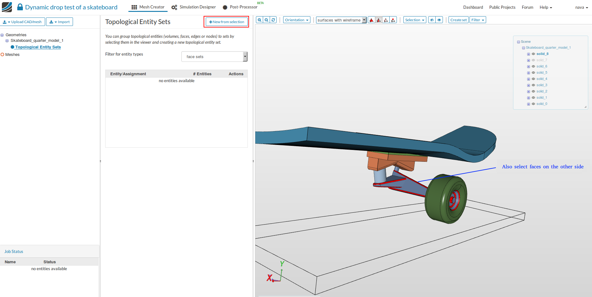
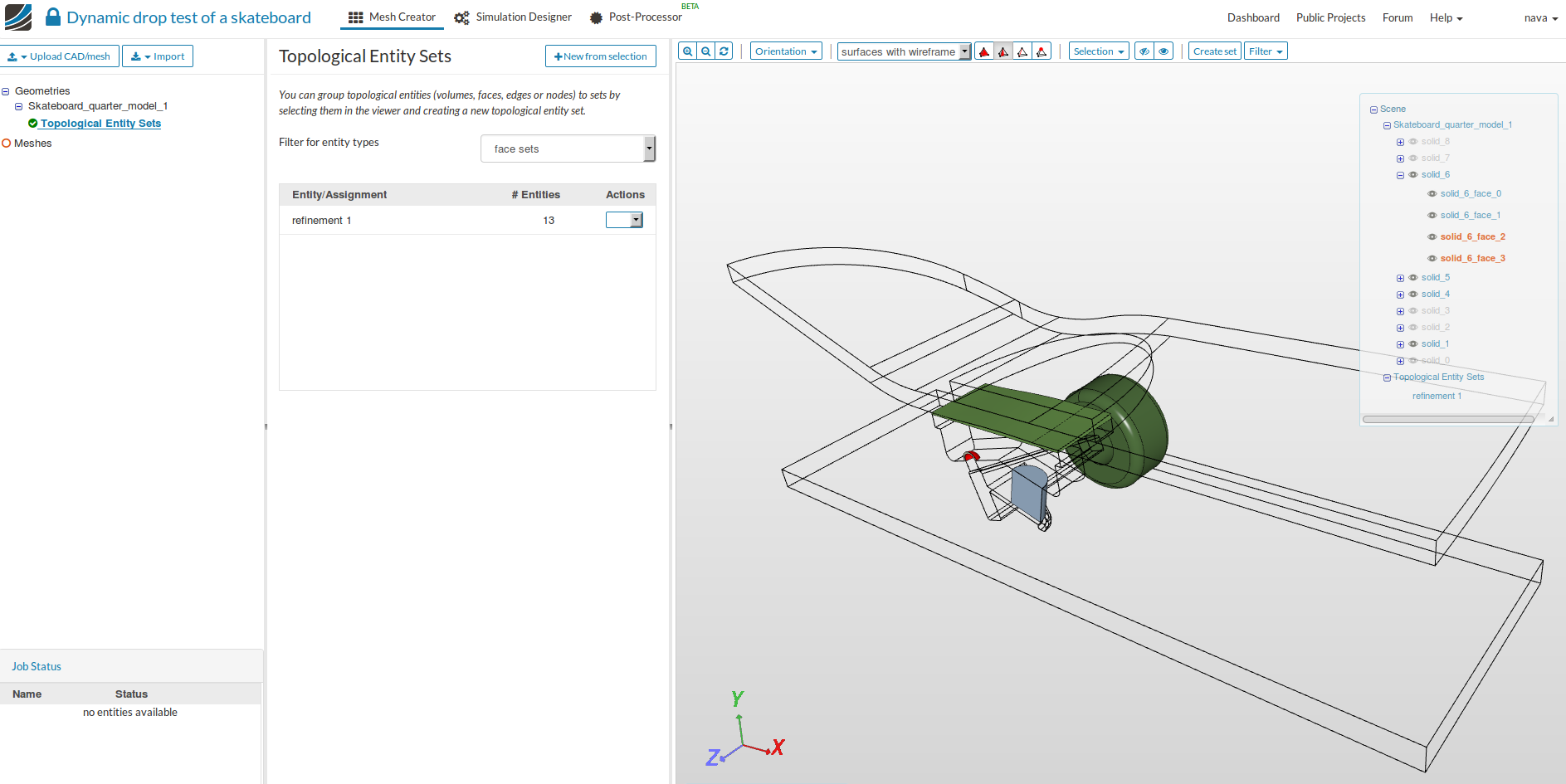
Here we are making set of faces having very small curved features (mostly small fillets). Select the faces shown in the figure and then click on New from selection. Give a suitable name e.g. refinement 1.

For the curved features larger than the previous set (mostly larger fillets) we will create another topological set by selecting the faces shown in figures below and then click on New from selection. Give a suitable name e.g. refinement 2.

You can check the selected faces for two topological sets against the table given below.

Now we have to mesh our geometry. Go to Skateboard_quarter_model_1 and click on ‘New Mesh’ button in the options panel.

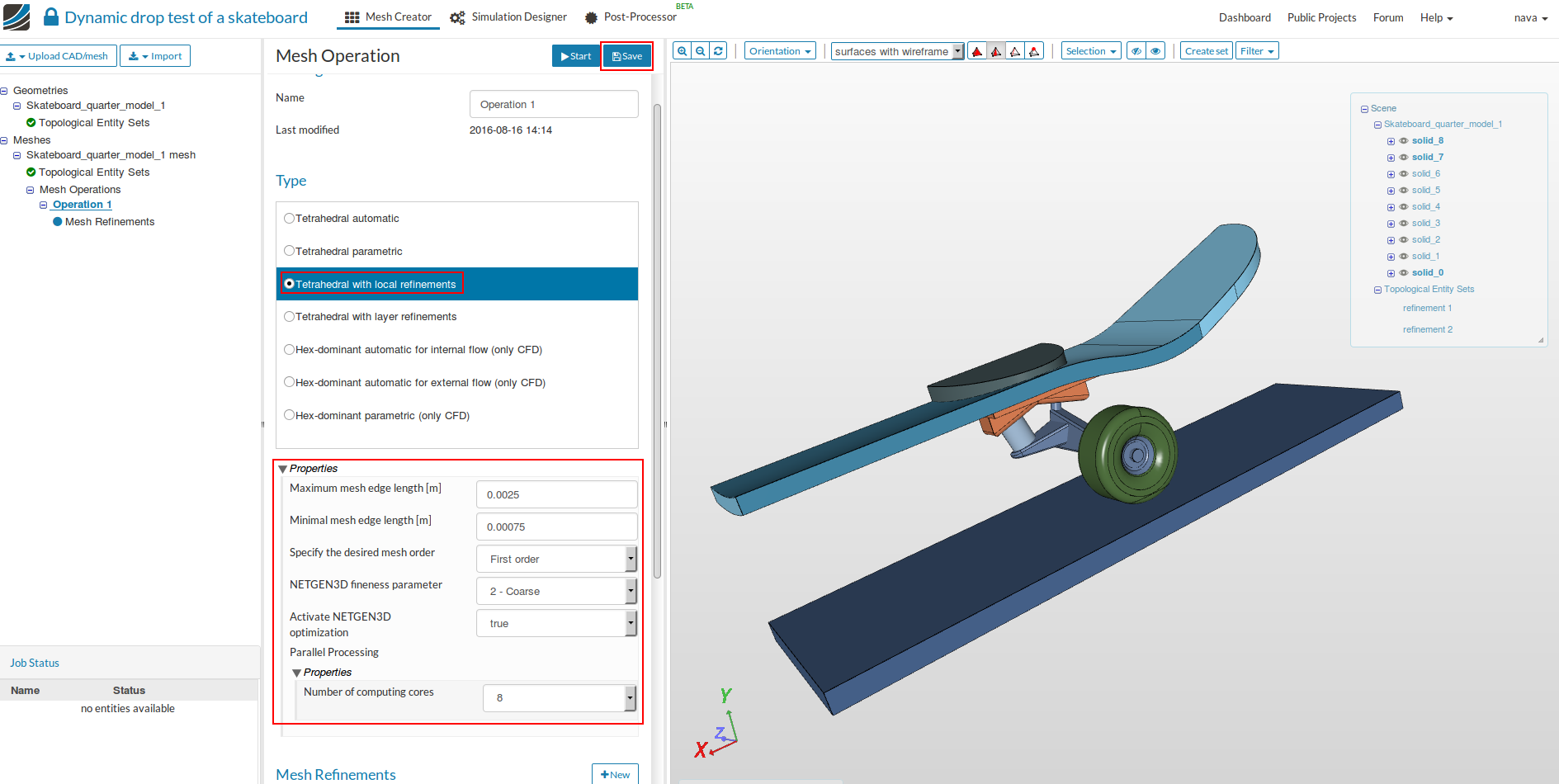
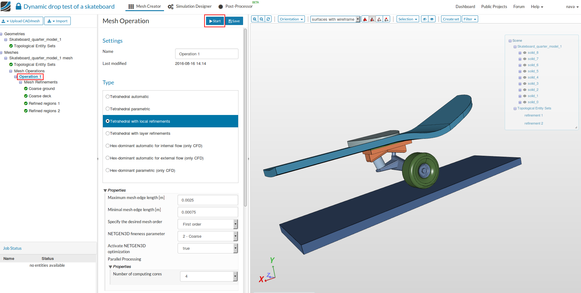
Select Tetrahedral with local refinement mesh and select the following parameters - 0.0025 and 0.00075 under Maximum and minimum edge length.First order under the desired mesh order, 2-Coarse for fineness and 8 computing cores.

Click on Save button to save all settings.
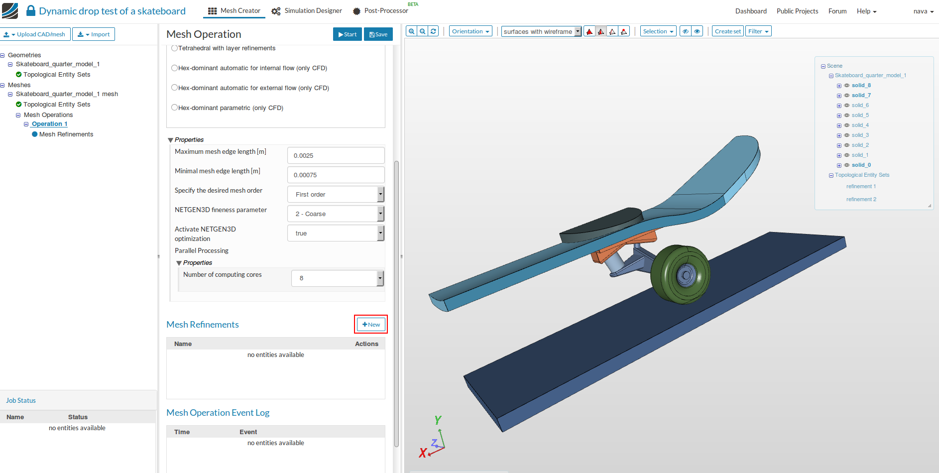
This defines the global settings of the mesh. Now we have to specify the local refinement based on the requirement.
Let’s start with the ground. Since the ground is rigid and the stresses on the ground is of no interest, we will make it very coarse compared to the global mesh size.
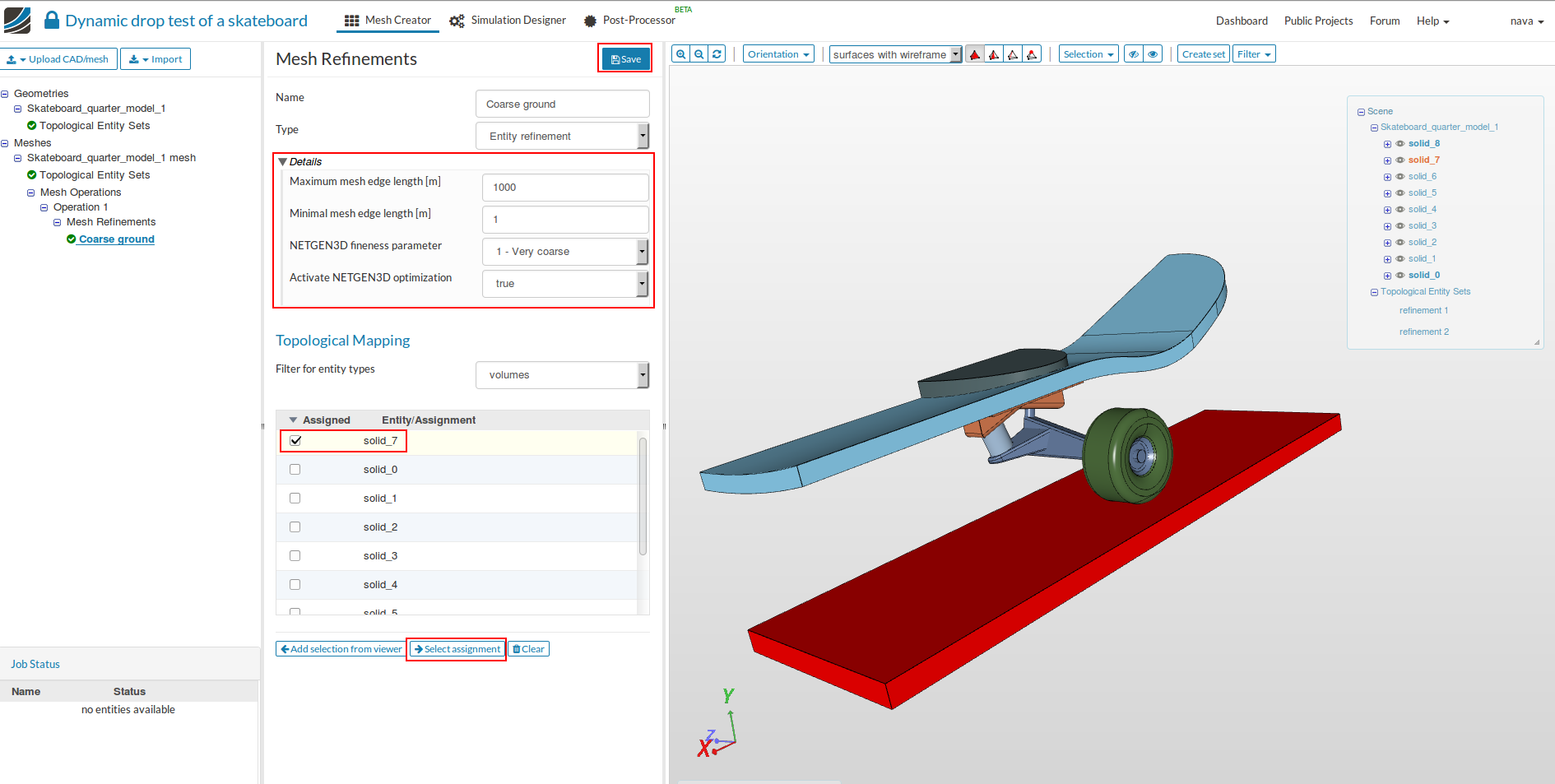
Create a refinement by clicking on New button.

Change the name of the refinement to a meaningful name e.g. Coarse ground (optional). Use all the settings given in the figure below. Use volumes for the ‘Filter for entities types’ under Topological Mapping, select solid_7 and then Save.
You can check for the selected volume by clicking on Select assignment. The assigned volume will be highlighted.

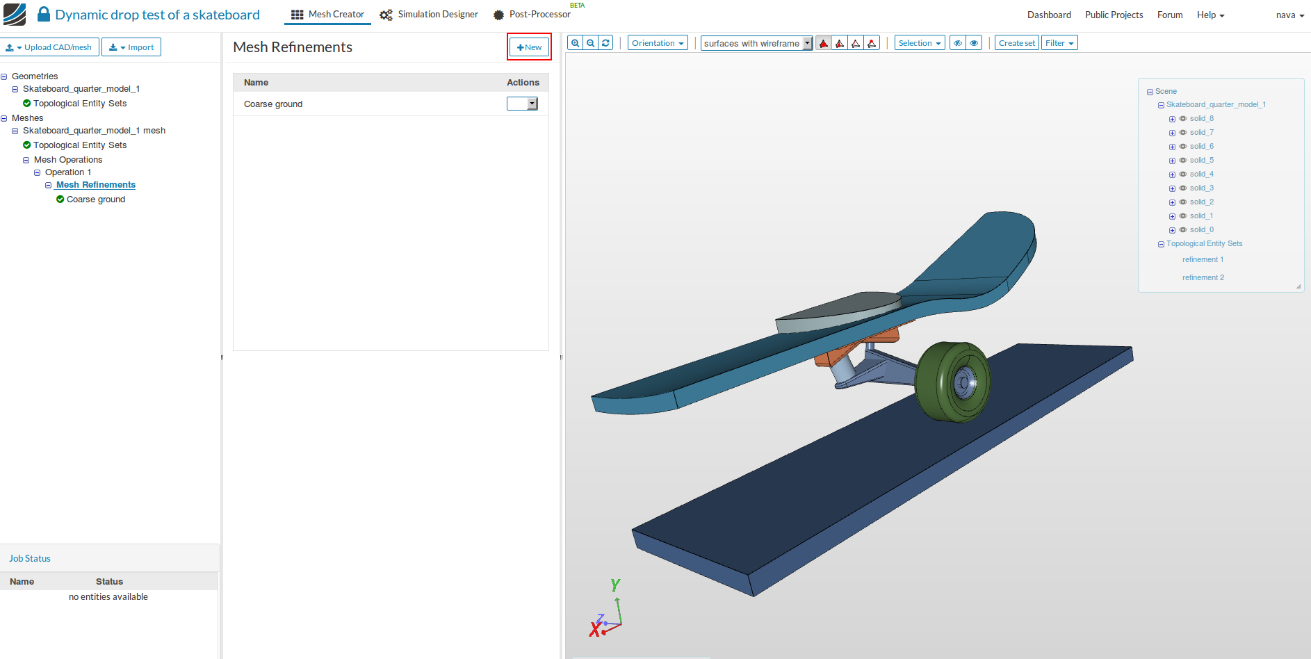
Create a new refinement by going back to Mesh Refinements and then click on New.

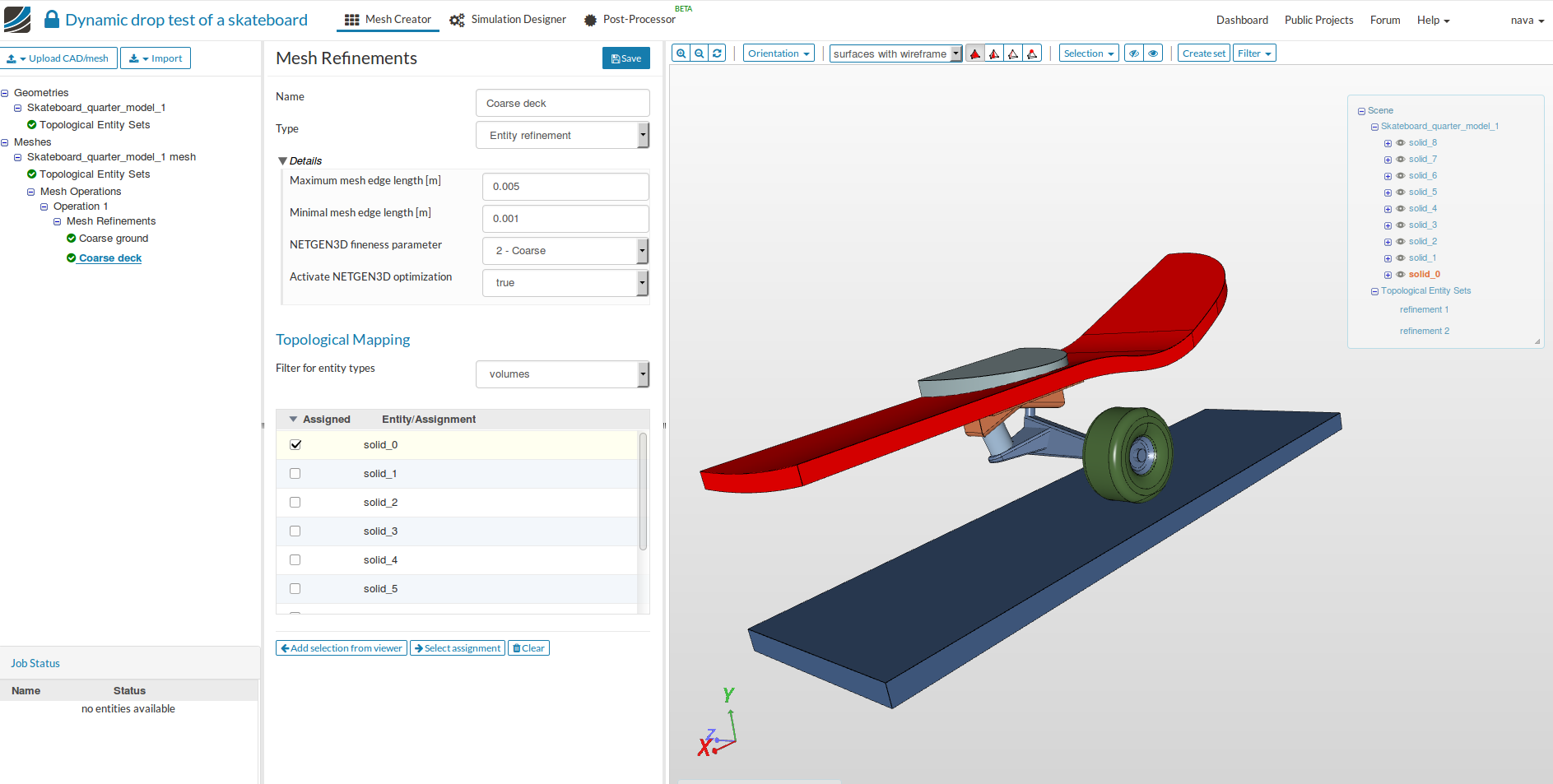
Now we are creating a coarse refinement for the skateboard’s deck as the stresses here won’t play an important role in the design.
Follow the same steps as above with the parameters given in the figure below. Give a suitable name to the refinement e.g. Coarse deck (optional). Select solid_0 (deck) and then Save.

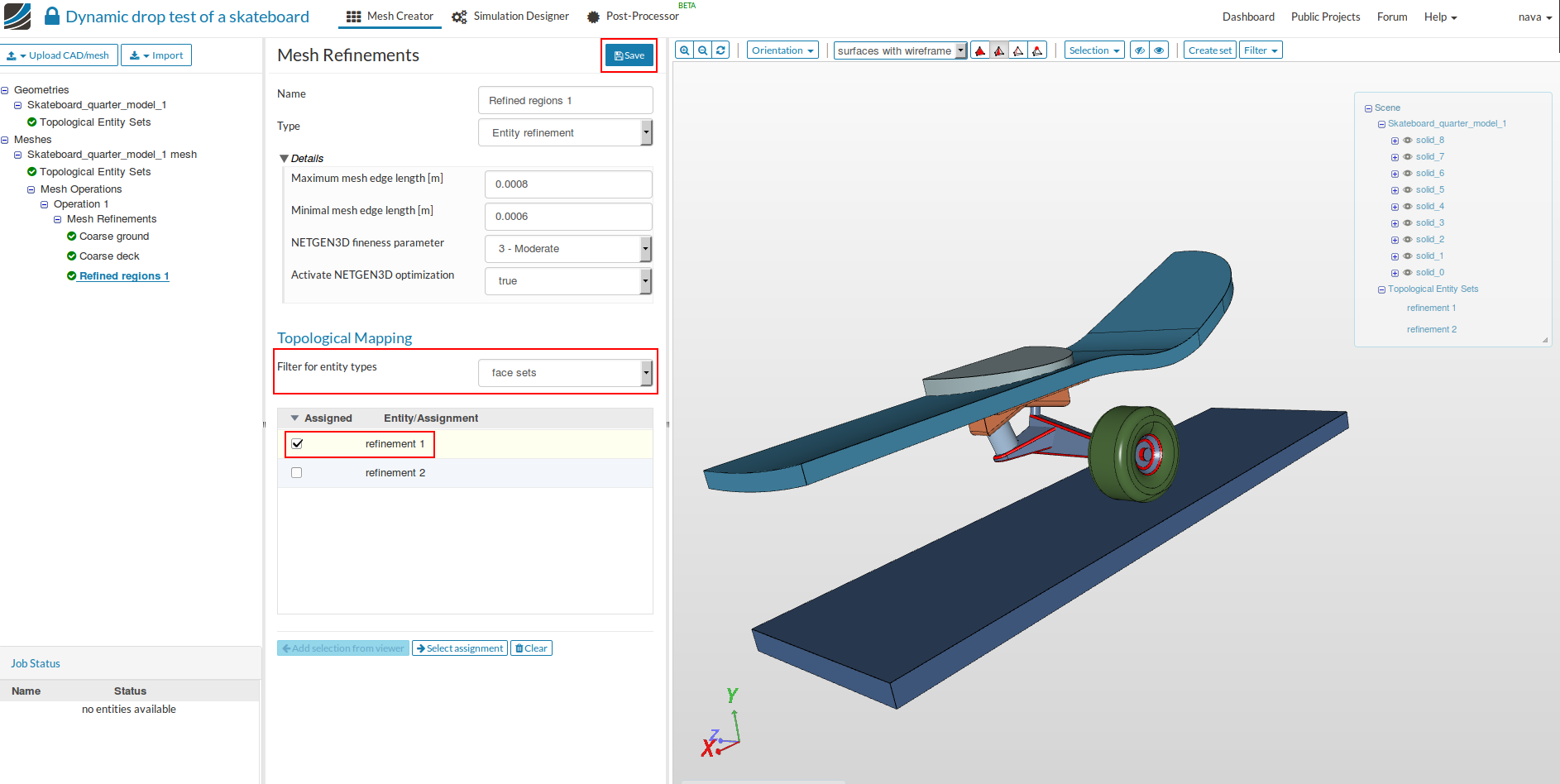
Now we are creating a local refinement to capture the small curved surfaces. Follow the same procedure as above to create a new refinement.
Give it a meaningful name e.g. Refined regions 1 (optional) and specify all the parameters given in the figure below. Change the ‘filter for entity types’ to face sets and choose refinement 1 and then Save.

Now we are creating a local refinement to capture relatively larger curved surfaces as compared to previous set. Follow the same procedure as above to create a new refinement.
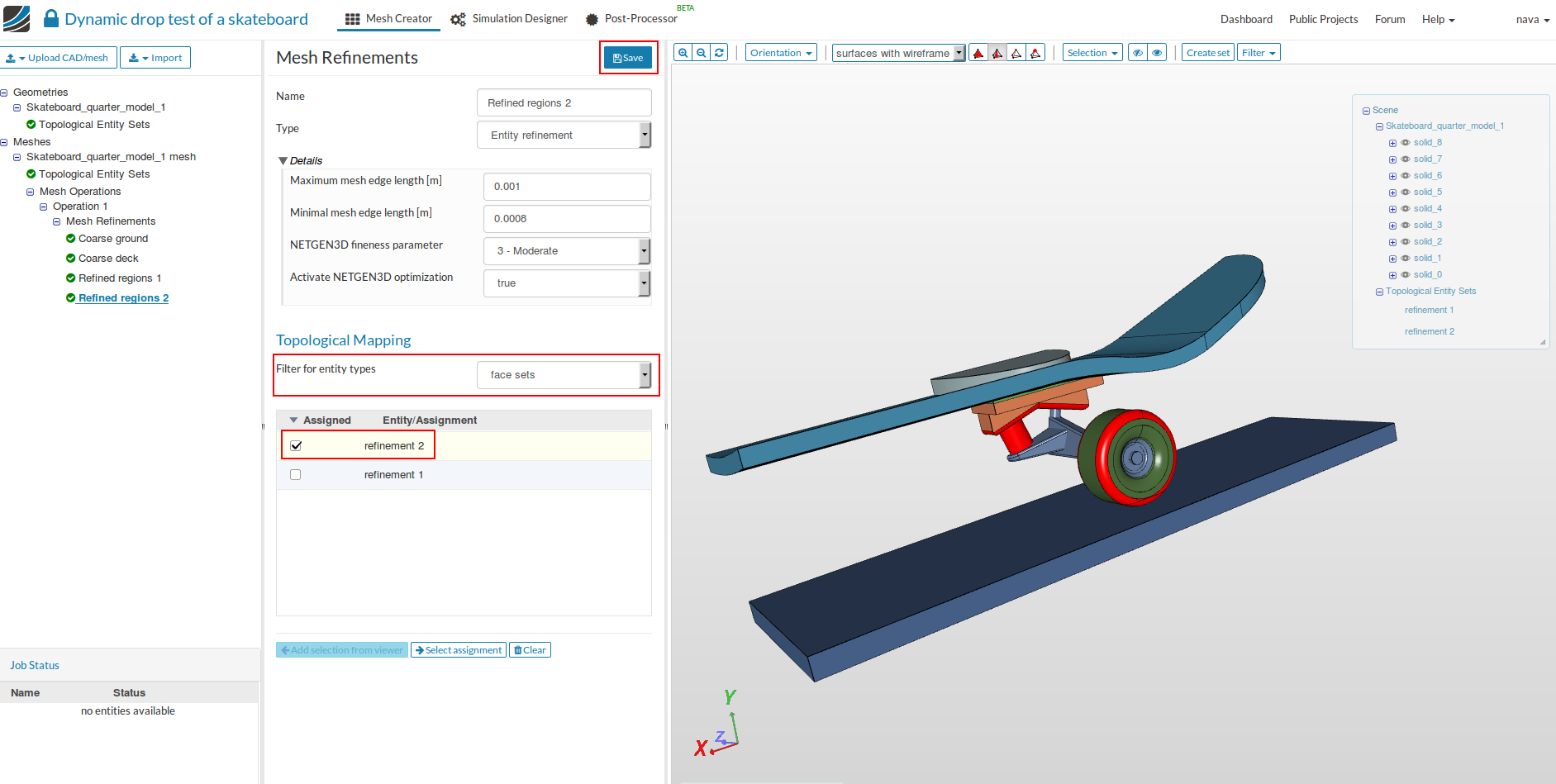
Give it a meaningful name e.g. Refined regions 2 (optional) and specify all the parameters given in the figure below. Change the ‘filter for entity types’ to face sets and choose refinement 2 and then Save.

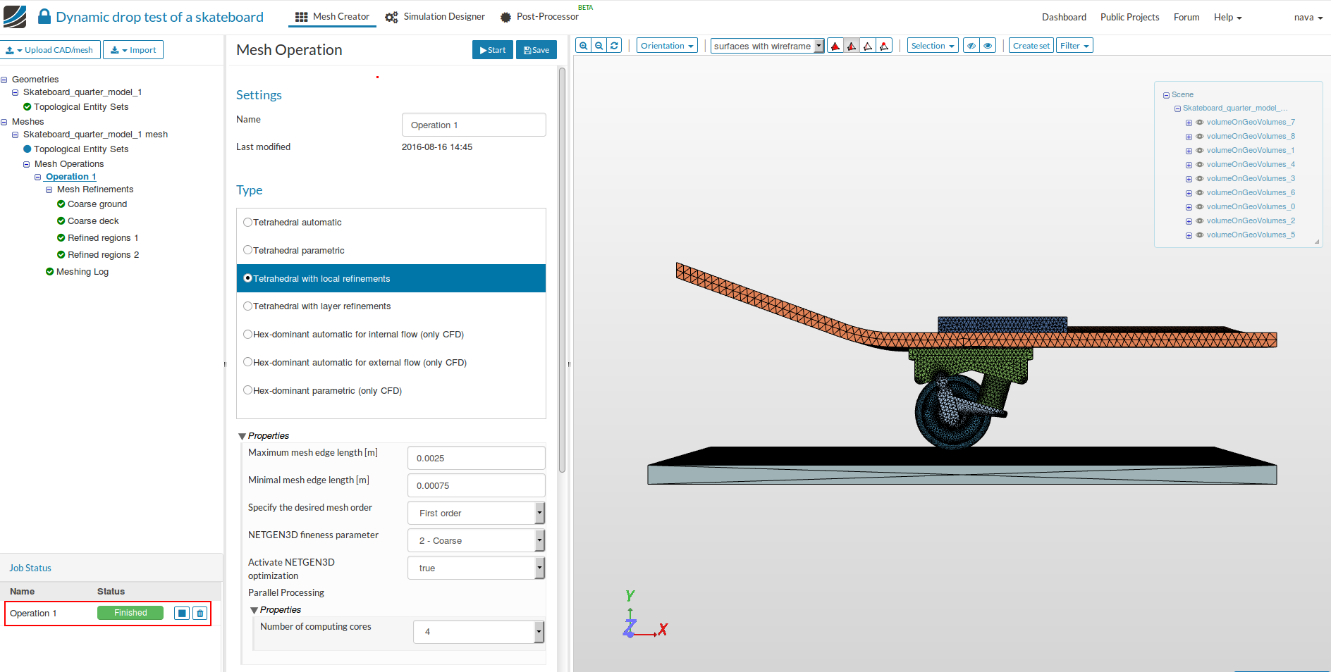
Now, we have defined all the mesh parameters. In order to start the meshing operation, go to Operation 1 and then click then Start.

The mesh operation takes about 5 minutes to complete and gives a ‘Finished’ status in the lower left once it is over.

Simulation Setup

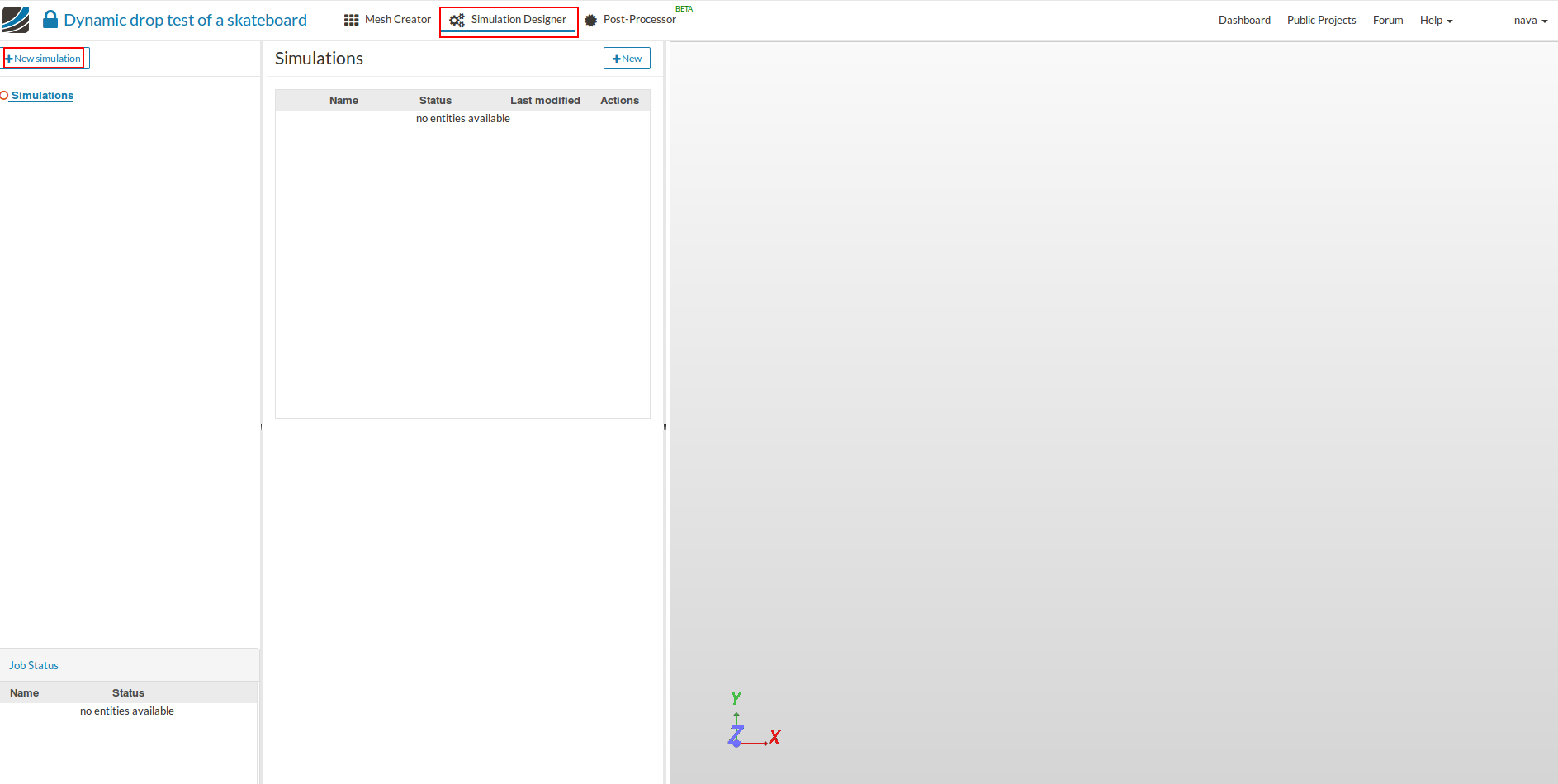
For setting up the simulation switch to the Simulation Designer tab and select New simulation.

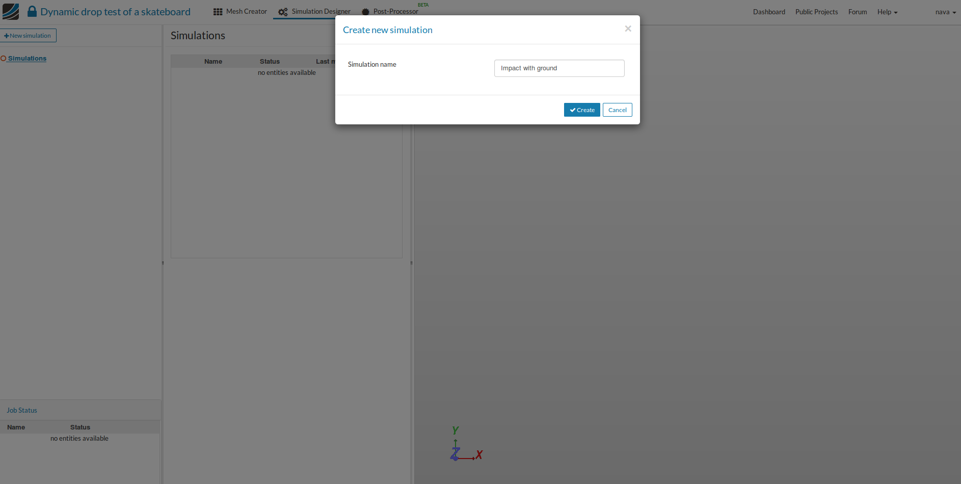
A create new project window will pop-up. Give a project suitable name (optional) e.g. Impact with ground in this case and click Create.

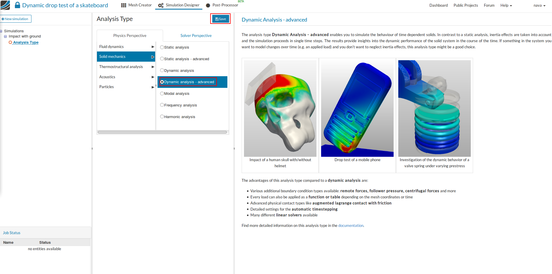
Since we are studying the impact of skate board with ground, select the analysis type Dynamic - advanced under Solid mechanics and click Save.

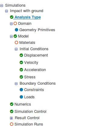
After saving, the simulation tree now looks as shown below. Here the Tree Entries in Red must be completed.

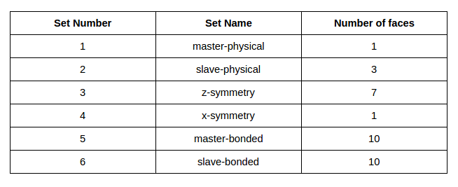
Domain selection

Click ‘Domain’ from the tree and select the mesh created from the previous task. Click the Save button. The mesh will then automatically load in the viewer.
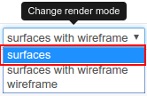
Furthermore, change render mode to ‘Surfaces’ on viewer top to interact with the mesh more easily.

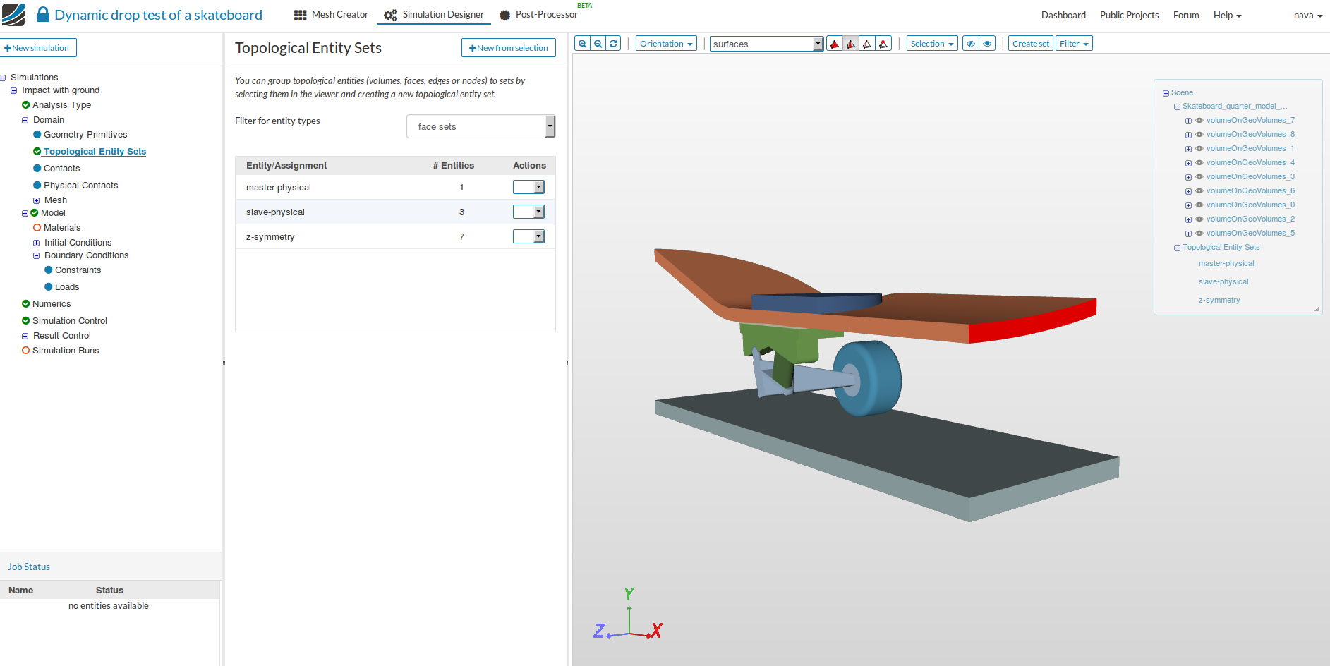
Create Topological Entity Sets

In this homework, we have several boundary conditions and contact definitions. An elegant way to apply these is by first creating a topological sets for different entities.
We will create 6 sets in total, as shown below:

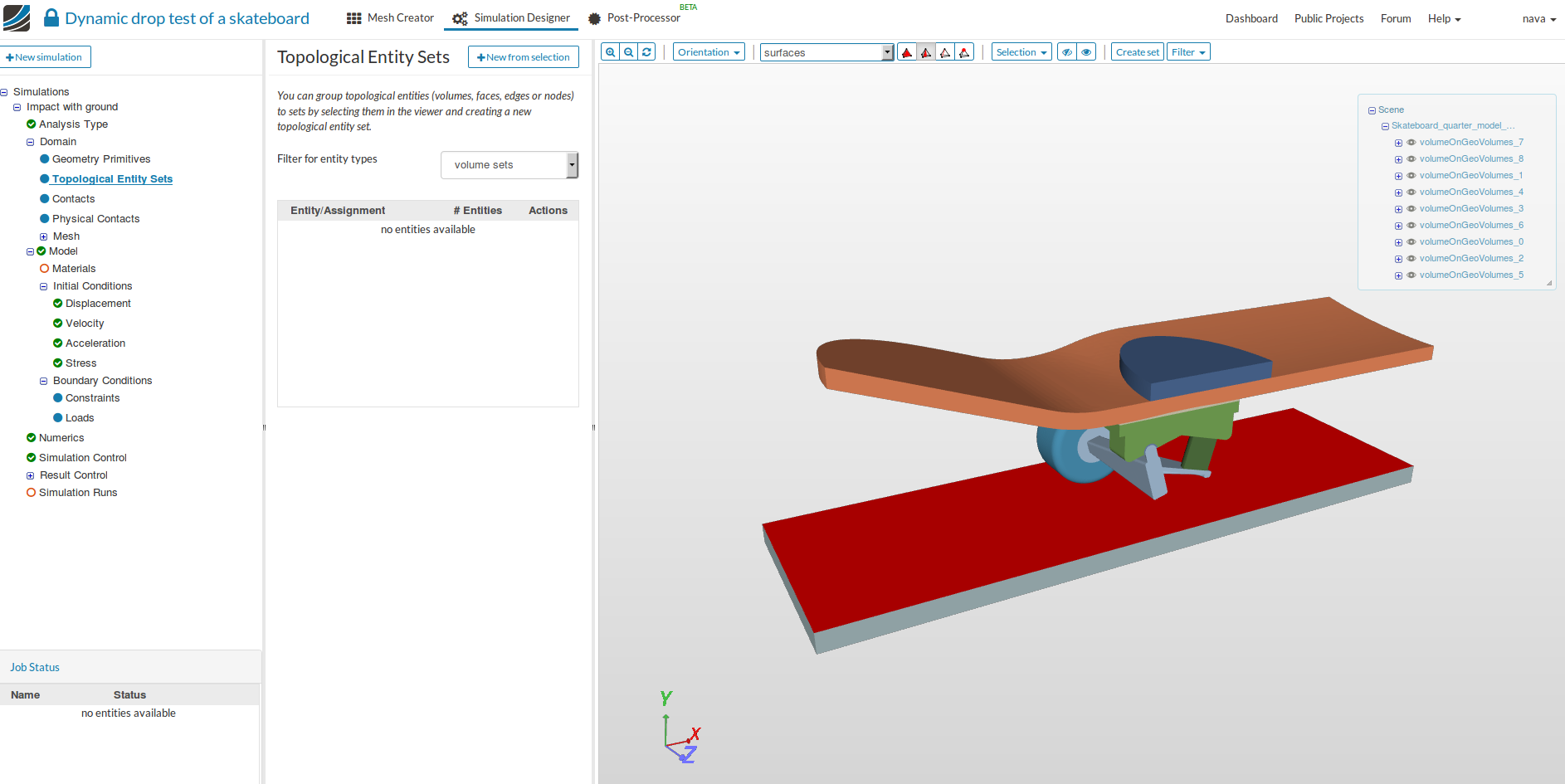
master-physical:

Click on the tree entry ‘Topological Entity Sets’.
For physical contact master surface, we will select the top face of the ground since it would be rigid making it best choice for the master entity (slave surfaces can not be fully constrained → leads to overconstrained system).
Next, click on New from selection, create set from the selection window will pop up, give it a meaningful name - master-physical and then click on Create.

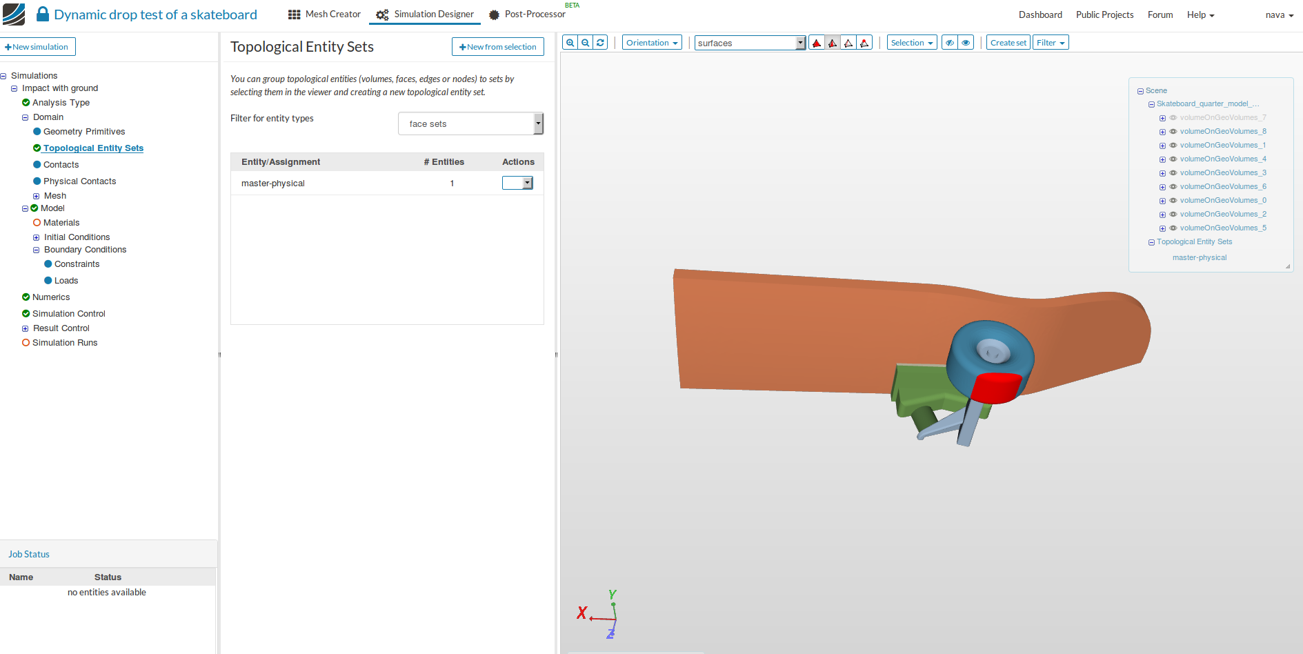
slave-physical:

To create the second set, select the face of the wheel which is contact with the ground, follow the same procedure as above to create a set named ‘slave-physical’.

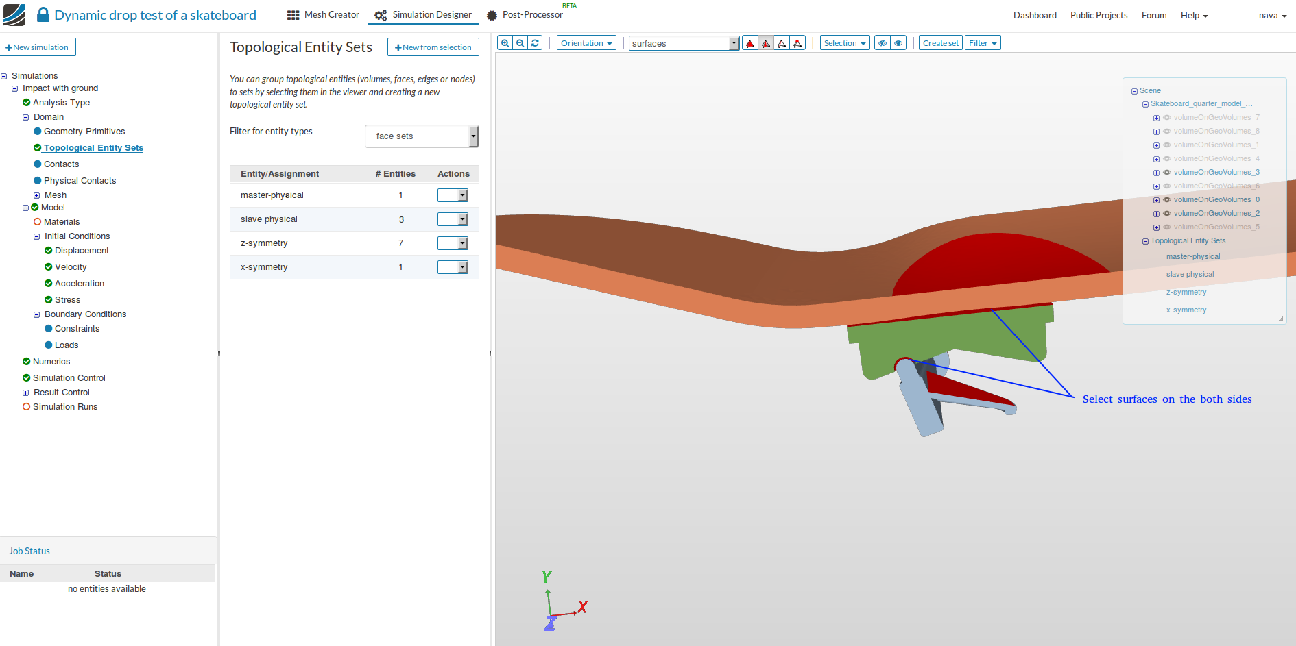
z-symmetry:

To create the third set, select the faces where you need to apply symmetry boundary conditions with respect to XY-plane and follow the same procedure as above to create a set named ‘z-symmetry’.

x-symmetry:

To create the fourth set, select the faces where you need to apply symmetry boundary conditions with respect to YZ-plane and follow the same procedure as above to create a set named ‘x-symmetry’.

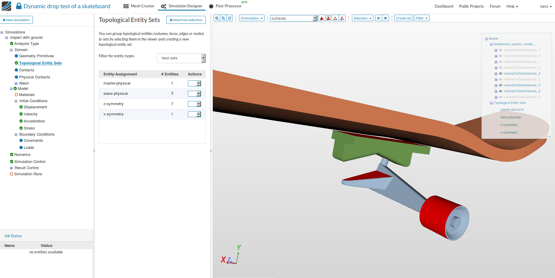
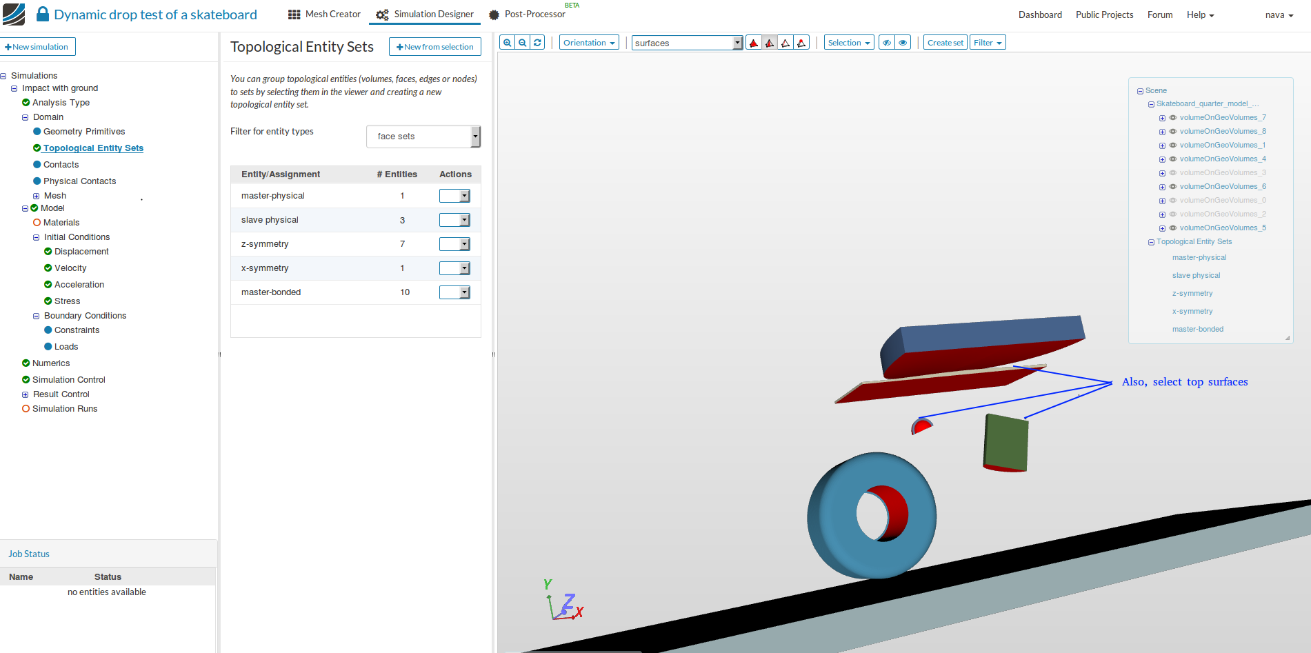
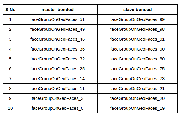
master-bonded:

Bonded contacts will be used to bond different material components with each other. Normally it’s always a good idea to make stiffer solid surfaces as master. Therefore, we will make the master bonded surfaces out of the following solids:
- deck (volumeOnGeoVolumes_0).
- truck upper (volumeOnGeoVolumes_2) portion.
- truck lower (volumeOnGeoVolumes_3) portion.
Hide all the other volumes except the above mentioned ones.
Next select the faces shown in the figures below and follow the same procedure as above to create a set named ‘master-bonded’.

(make sure you are in Pick faces mode before the selection , otherwise you would not be able to select the faces.)

slave-bonded:

Contrary to the master surfaces, now we will select the slave surfaces from the solids which will be considered bonded to those out of which master surfaces were made. In this case, they will be softer material solids i.e.
- polyurethane wheel (volumeOnGeoVolumes_5).
- bolted polyurethane between truck upper and lower portion (volumeOnGeoVolumes_4).
- polyurethane gasket between truck upper and lower portion (volumeOnGeoVolumes_6).
- polyurethane gasket between truck and deck (volumeOnGeoVolumes_1).
- rubber foot (volumeOnGeoVolumes_8).
Hide all the other volumes except the above mentioned ones.
Select the faces shown in the figures below and follow the same procedure as above to create a set named ‘slave-bonded’.

(make sure you are in Pick faces mode before the selection , otherwise you would not be able to select the faces.)

You can check the list of faces you have selected for master-bonded and slave bonded against the table given below.

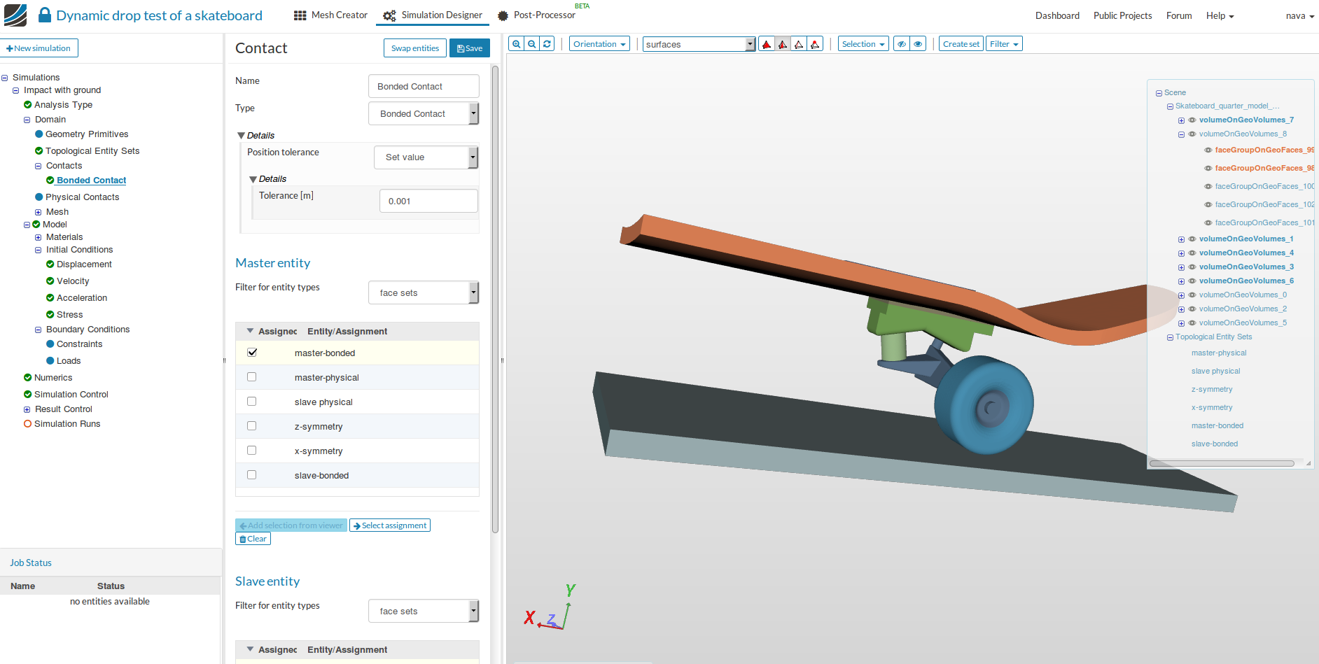
Contacts

Here we will define the bonded contact between all components of the assembly.
Select ‘Contacts’ from the sub-tree and click New.

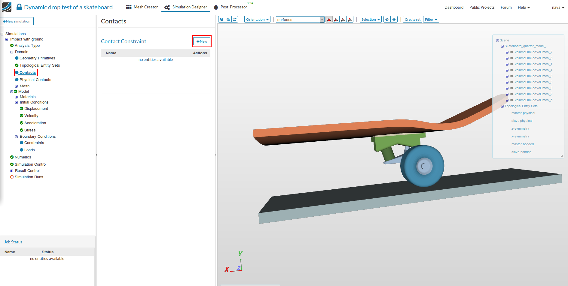
Give a suitable name - Bonded Contact (optional).
Select Bonded contact under type and choose master-bonded and slave-bonded topological sets for Master and Slave entity, respectively. Click Save.

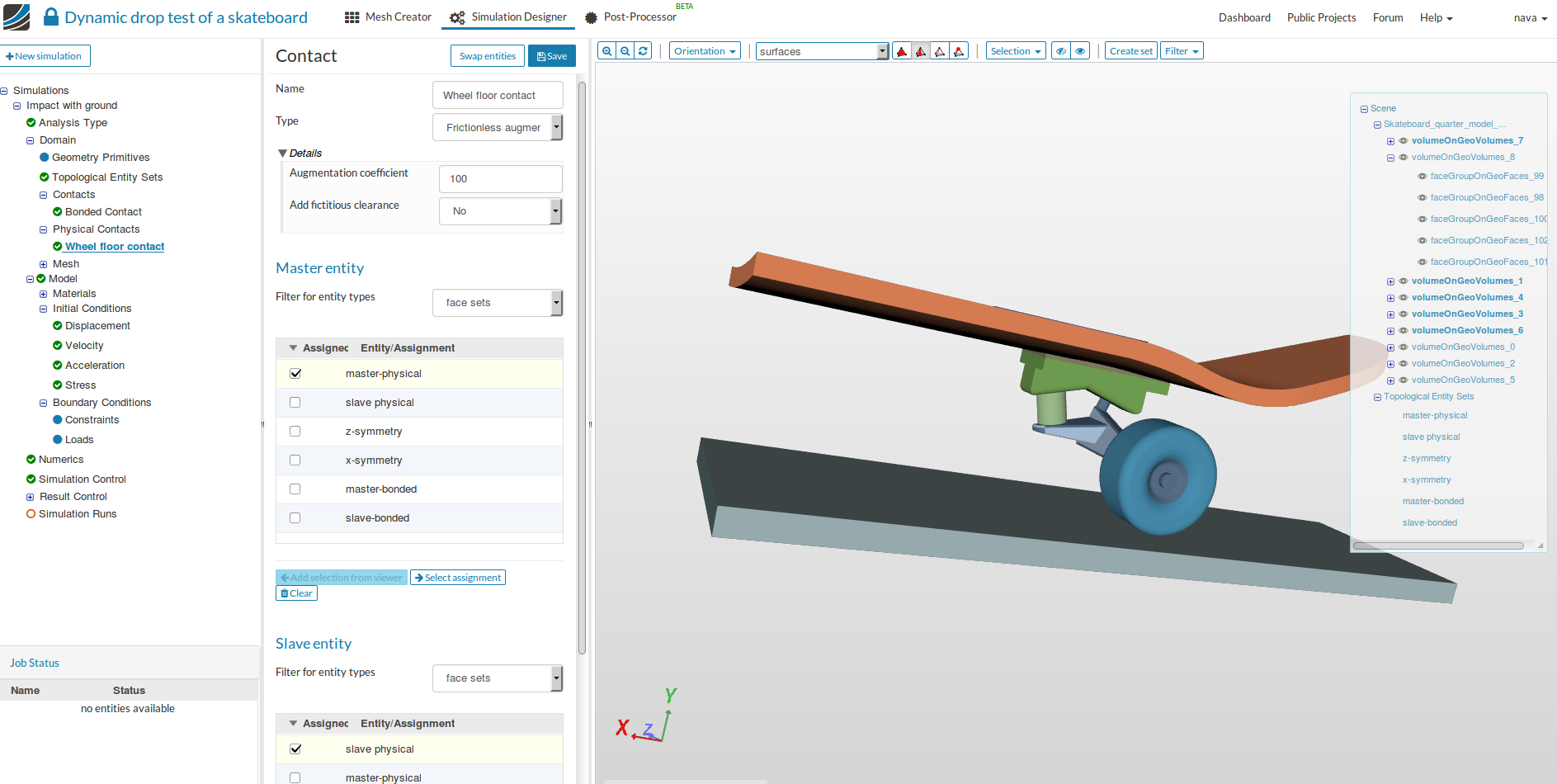
Physical Contacts

Having defined the bonded contact between all the components that are in contact, we also need to define a contact between the wheel and the ground.
Select ‘Physical Contacts’ from the sub-tree, choose Augmented Lagrange for Solution method click Save and then New

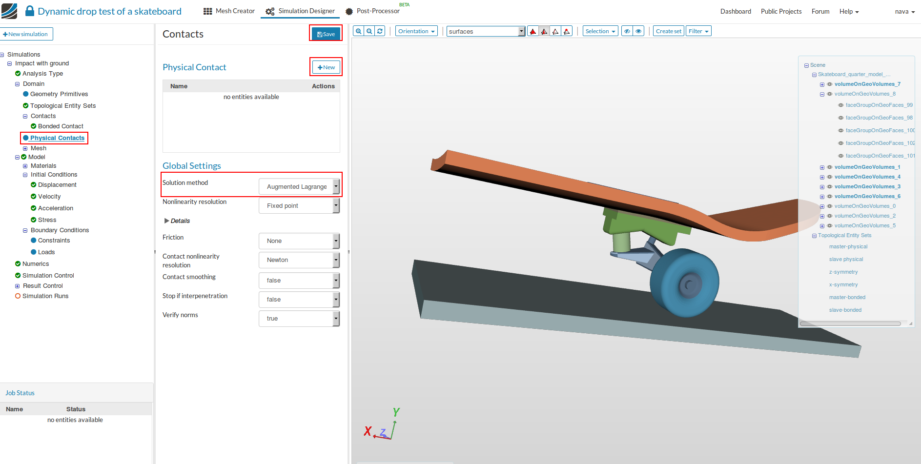
Give a suitable name - Wheel floor contact (optional). Select Frictionless augmented Lagrange contact under type and choose master-physical and slave-physical topological sets for Master and Slave entity, respectively.Click Save.

Select Solid Materials

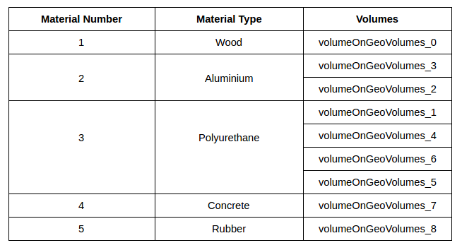
Now we will define materials for different components of the skateboard. We are using 5 different materials for our simulations as shown in the figure below.

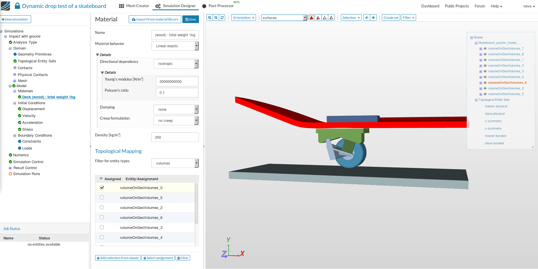
Deck (wood) - total weight 1kg:

Select ‘Material’ from the sub-tree and click New.

Change:
Name to Deck (wood) - total weight 1kg (optional).
Young’s Modulus [N/m²] to 20000000000 (defines the stiffness of the material).
Poisson’s ratio to 0.1 (defines the relationship between deformation of a material along perpendicular axis).
Density [kg/m³] to 250 (defines the self load of the geometry).
Select the volume under Topological Mapping , select volumeOnGeoVolumes_0 and click Save.

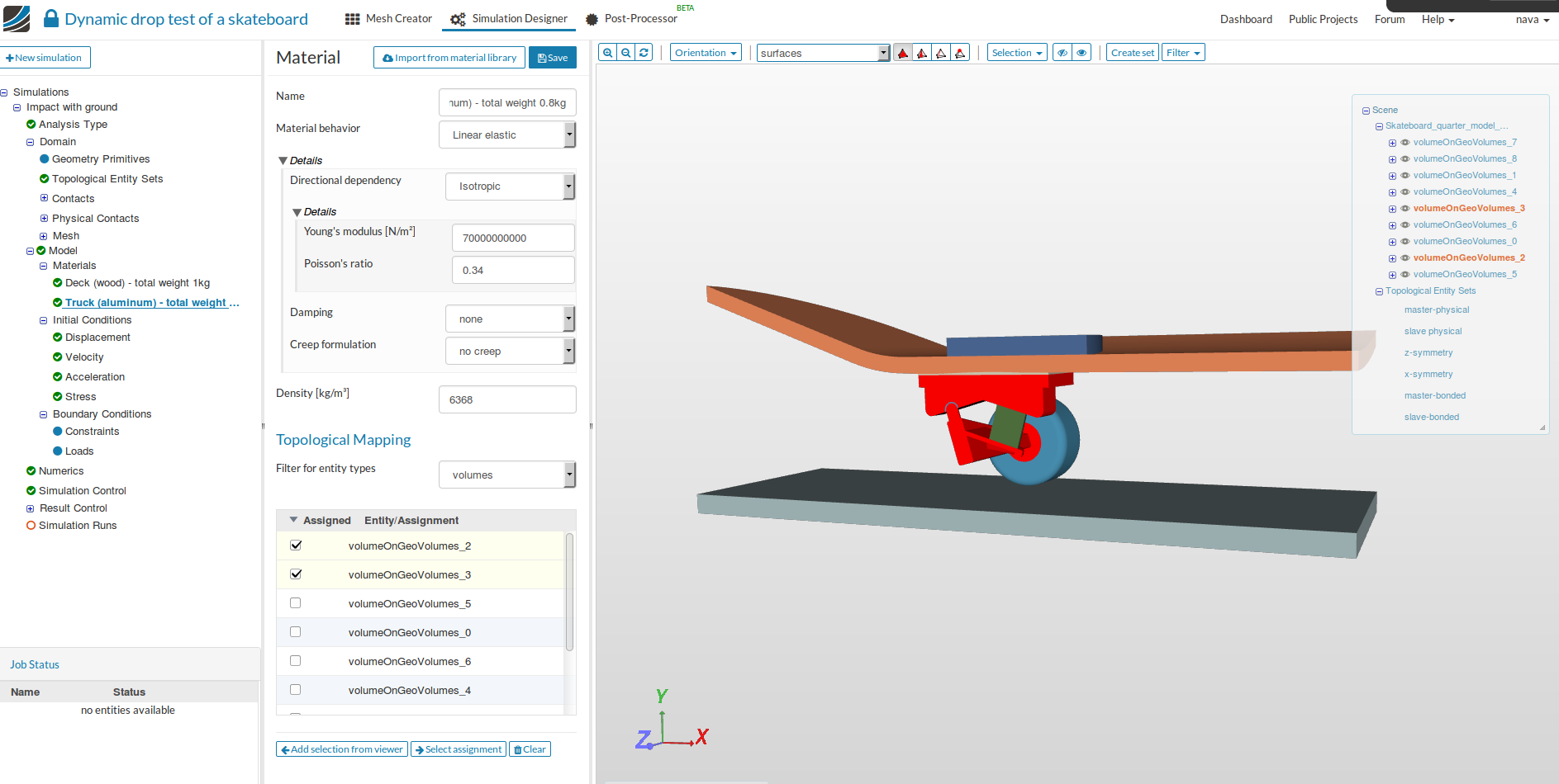
Truck (aluminum) - total weight 0.8kg:

Follow the same step as above to create a new material.
Change:
Name to Truck (aluminum) - total weight 0.8kg (optional).
Young’s Modulus [N/m²] to 70000000000 (defines the stiffness of the material).
Poisson’s ratio to 0.34 (defines the relationship between deformation of a material along perpendicular axis).
Density [kg/m³] to 6368 (defines the self load of the geometry).
Select the volume under Topological Mapping , select volumeOnGeoVolumes_2 and volumeOnGeoVolumes_3. Click Save.

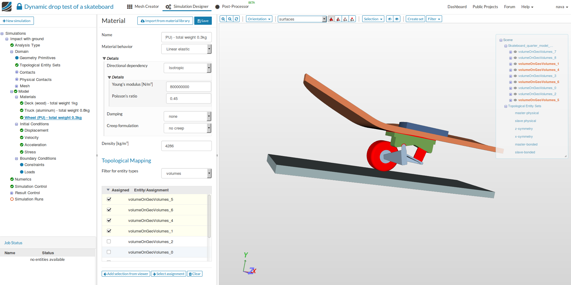
Wheel (PU) - total weight 0.3kg :

Follow the same step as above to create a new material.
Change:
Name to Wheel (PU) - total weight 0.3kg (optional).
Young’s Modulus [N/m²] to 800000000 (defines the stiffness of the material).
Poisson’s ratio to 0.45 (defines the relationship between deformation of a material along perpendicular axis).
Density [kg/m³] to 4286 (defines the self load of the geometry).
Select the volume under Topological Mapping , select volumeOnGeoVolumes_1 ,volumeOnGeoVolumes_4, volumeOnGeoVolumes_5 and volumeOnGeoVolumes_6. Click Save.

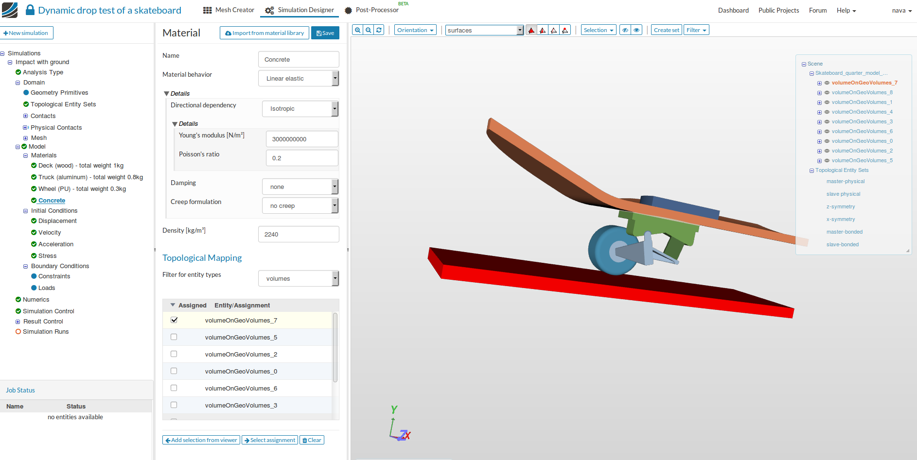
Concrete:

Follow the same step as above to create a new material.
Change:
Name to Concrete (optional).
Young’s Modulus [N/m²] to 3000000000 (defines the stiffness of the material).
Poisson’s ratio to 0.2 (defines the relationship between deformation of a material along perpendicular axis).
Density [kg/m³] to 2240 (defines the self load of the geometry).
Select the volume under Topological Mapping , select volumeOnGeoVolumes_7 and Click Save.

Foot (rubber) - total weight 32.5kg:

Follow the same step as above to create a new material.
Change:
Name to Foot (rubber) - total weight 32.5kg (optional).
Young’s Modulus [N/m²] to 200000000 (defines the stiffness of the material).
Poisson’s ratio to 0.48 (defines the relationship between deformation of a material along perpendicular axis).
Density [kg/m³] to 349462 (defines the self load of the geometry).
Select the volume under Topological Mapping , select volumeOnGeoVolumes_8 and Click Save.

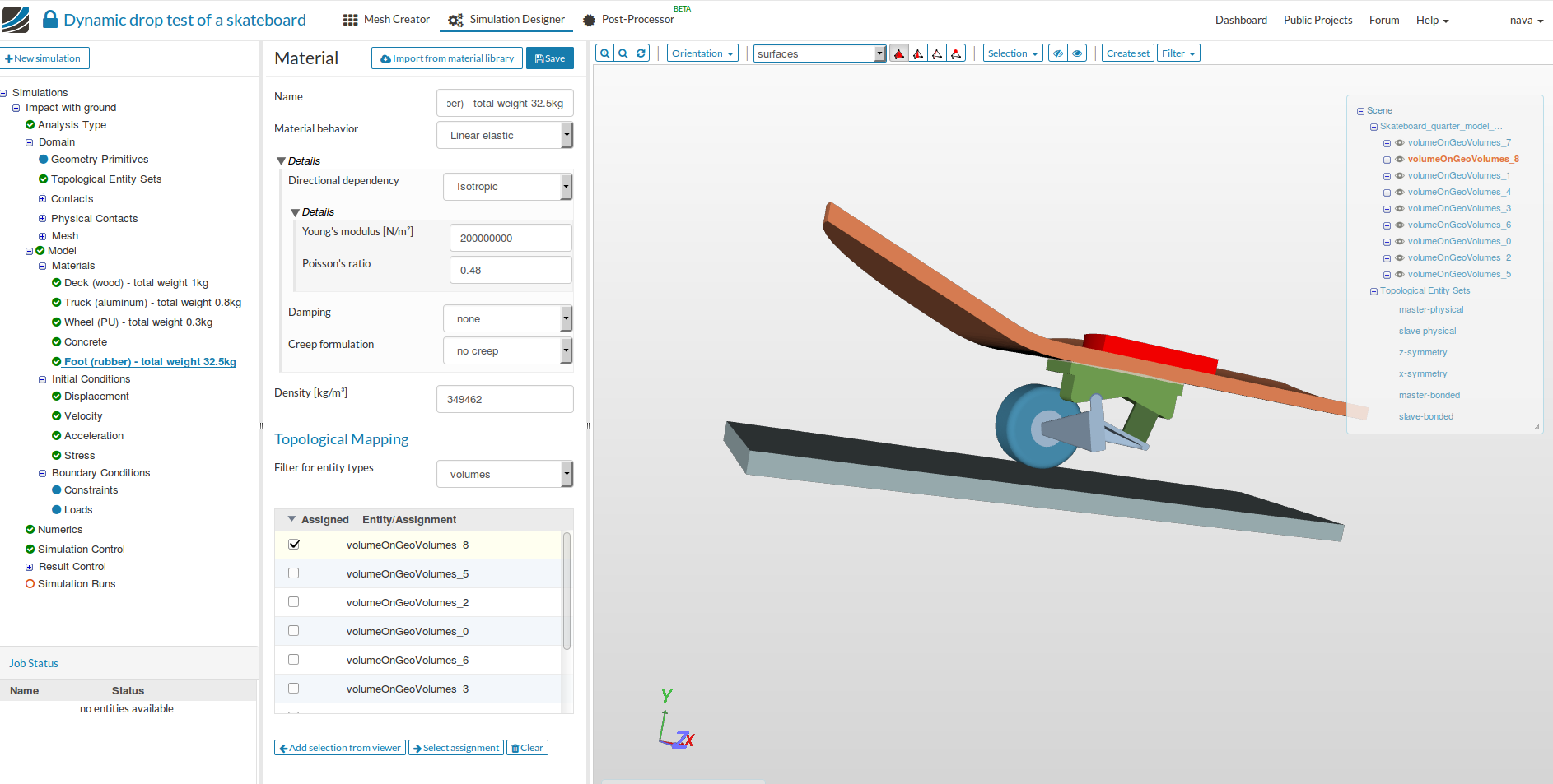
Note: The density of the rubber given here is not the actual density. It is calculated by dividing an average human’s weight (65 kg) by the total volume of the rubber in order to account for the dynamic load due to body weight .

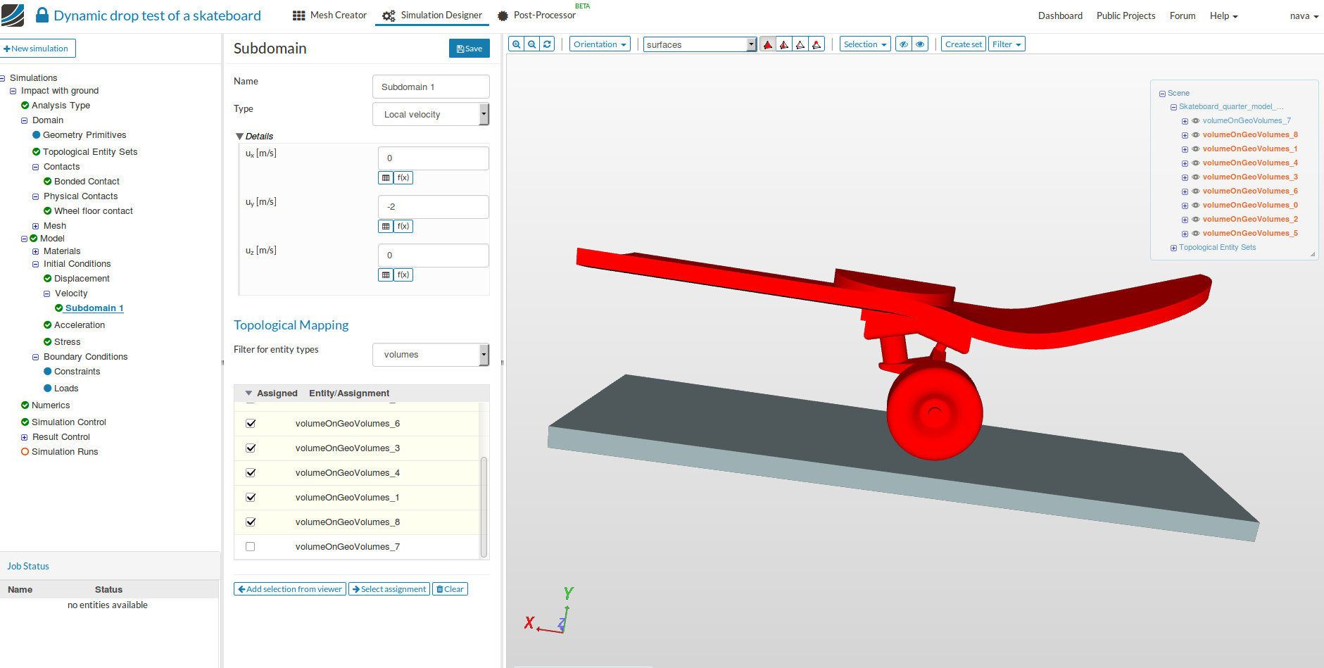
Initial Conditions

In this section we will define the dropping velocity of the skateboard with respect to ground.

Select Velocity under Initial Velocity in the tree.
Choose Subdomain-based as Type and then Save.

Click on New, specify uy equal to -2 and select all the volumes except volumeOnGeo_7.

Boundary Conditions

In this section we will define symmetry conditions and fixation of the ground. First we will define symmetry normal to z axis (XY-plane).

z-symmetry:

Select Constraint under Boundary Conditions in the tree and click on New to create a new constraint.

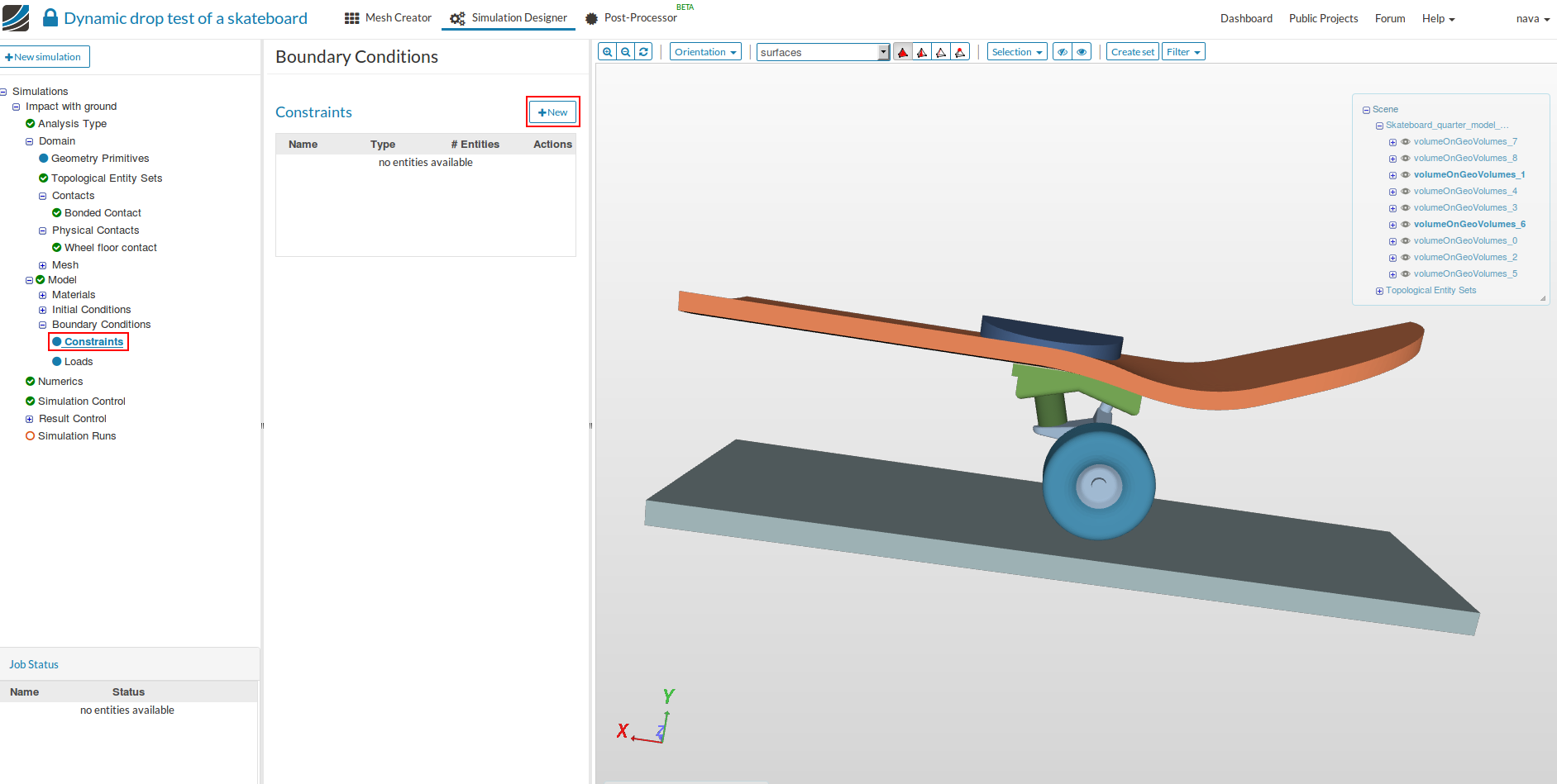
Choose unconstrained for x and y displacement and specify 0 for z-displacement.
Choose face sets under Topological Mapping, then choose z-symmetry topological set and finally Save.

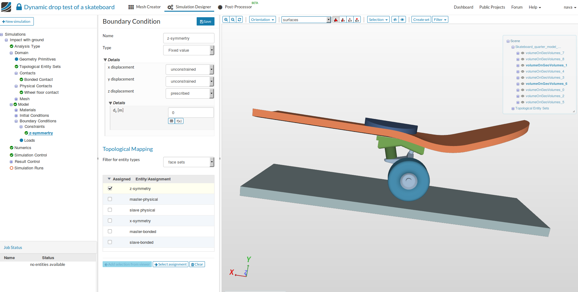
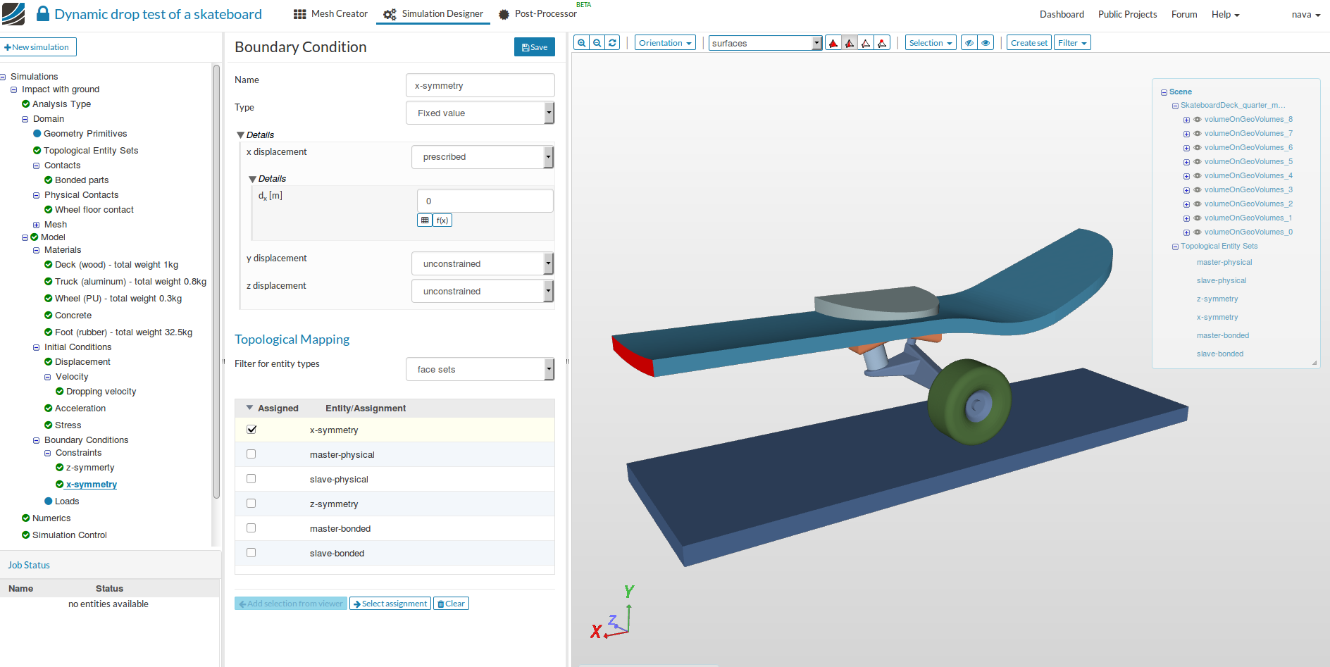
x-symmetry:

For applying symmetry about YZ-plane, follow same steps as above except here x-displacement will be specified as 0 and x-symmetry topological set will be selected.

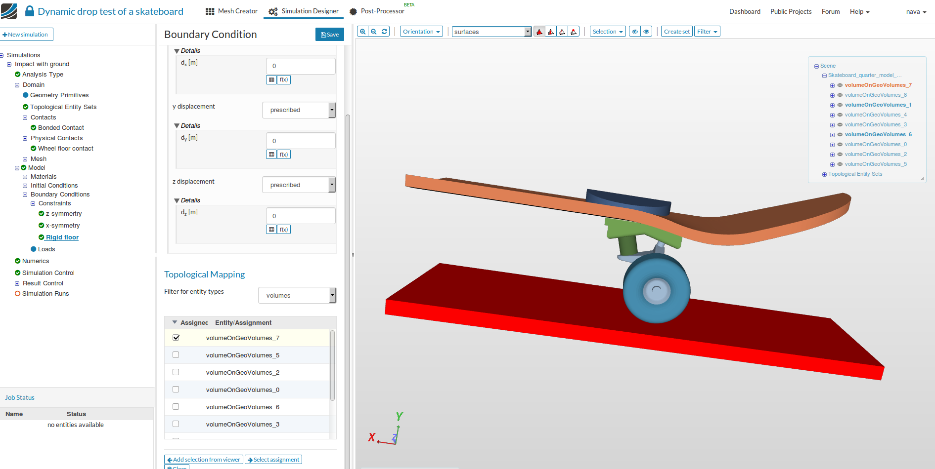
Rigid floor:

For applying fixation to the ground, follow same steps to create a new constraint.
Change the name to Rigid floor (optional), Specify 0 for all displacements, select VolumeOnGeoVolumes_7 and then Save.

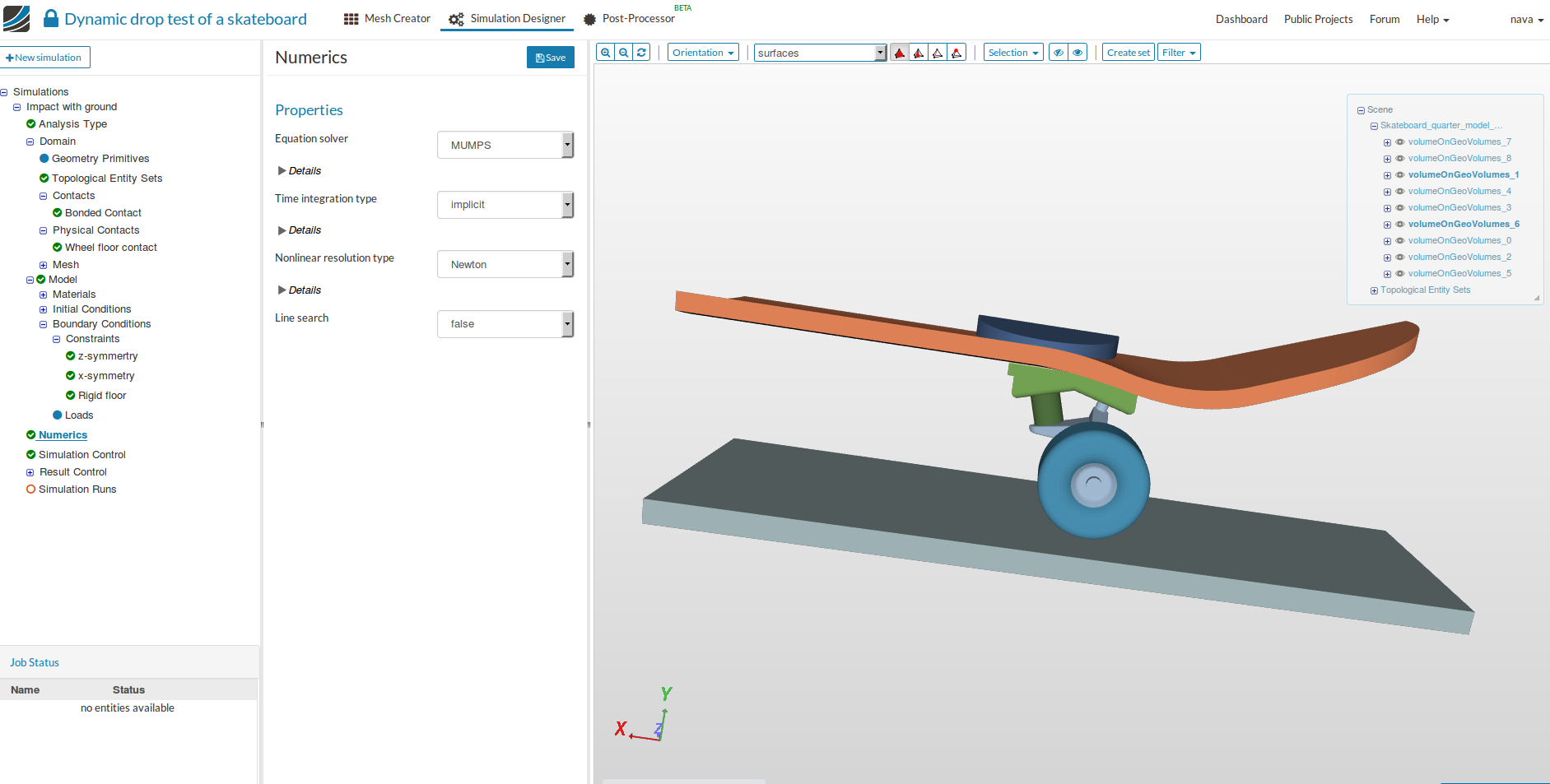
Numerics

Here we will select the solver type. For this simulation select MUMPS as Equation solver.

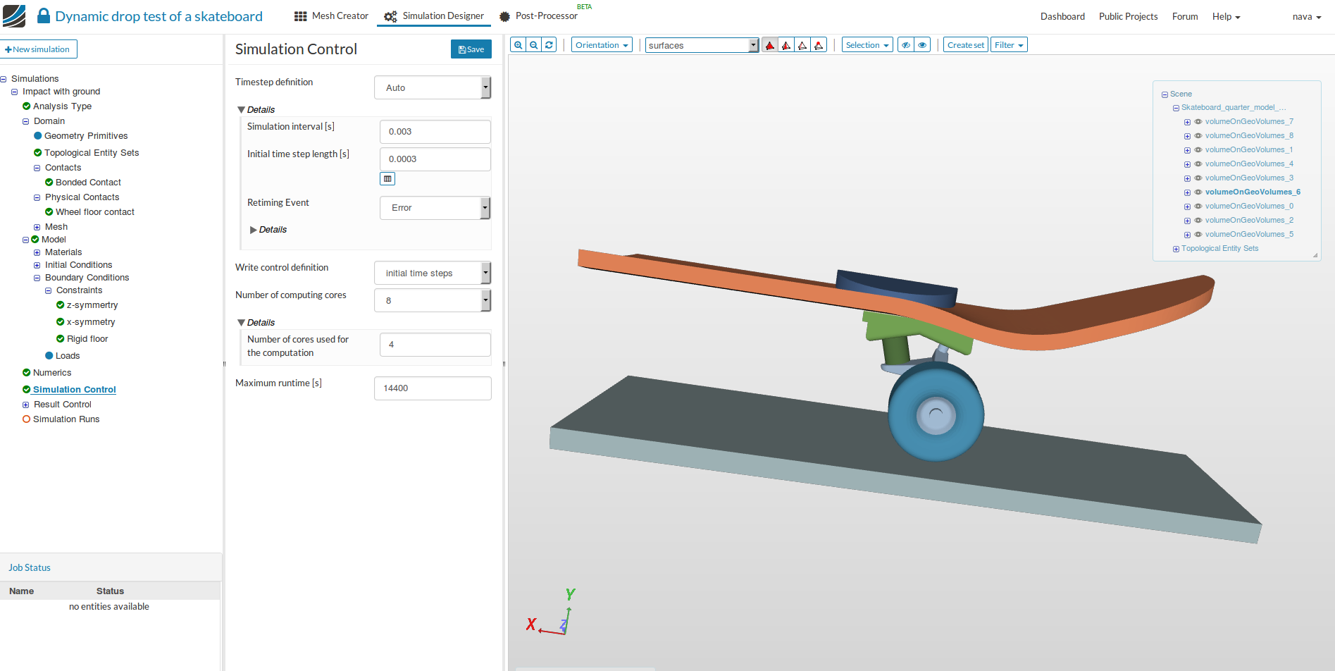
Simulation Control

Click on Simulation control and change Simuation interval [s] to 0.003 Initial time step length [s] to 0.0003 under details of Timestep definition, Number of computing cores to 8,Number of cores used for the computation to 4 and Maximum runtime [s] to 14400.

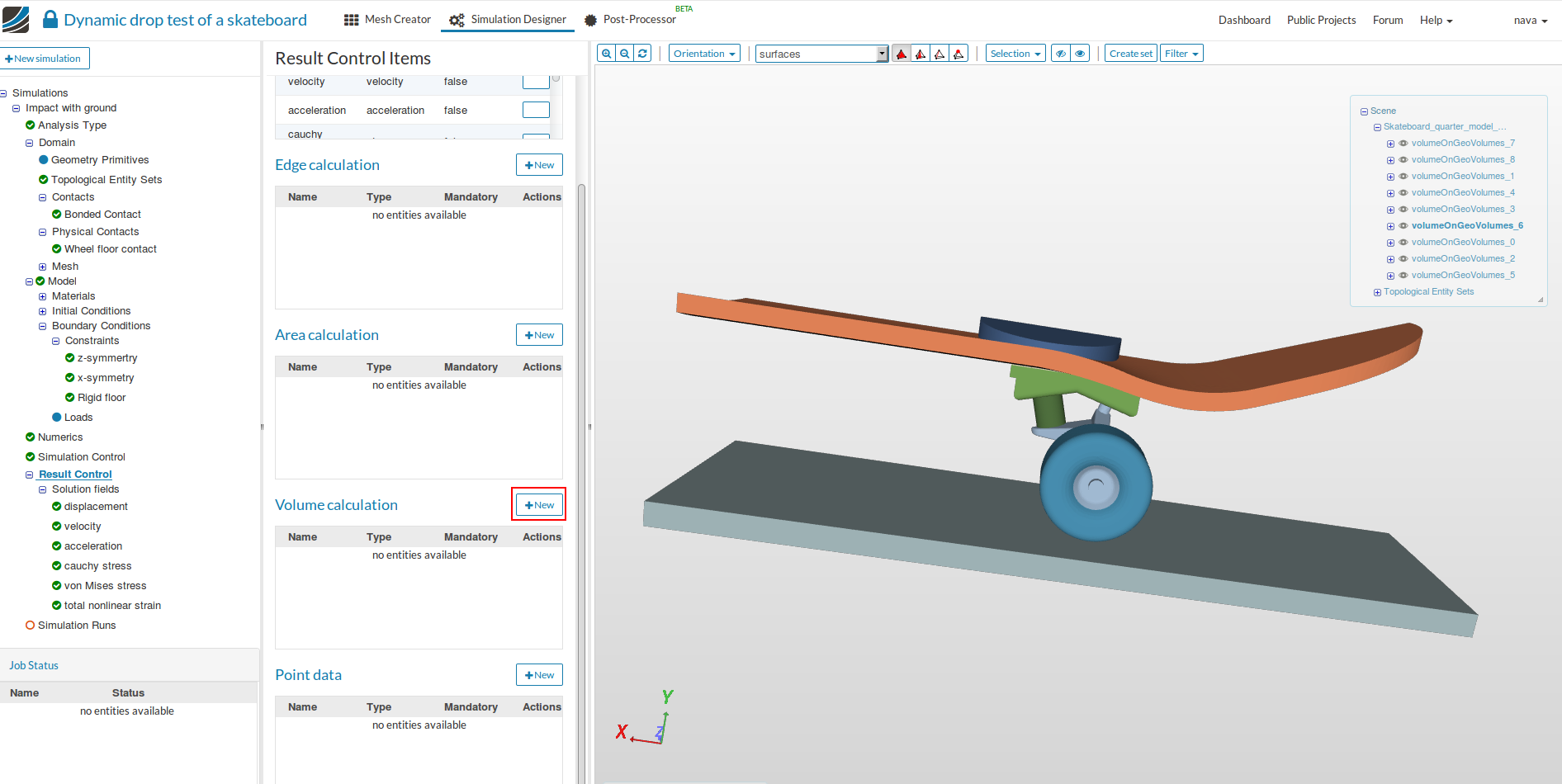
Result control

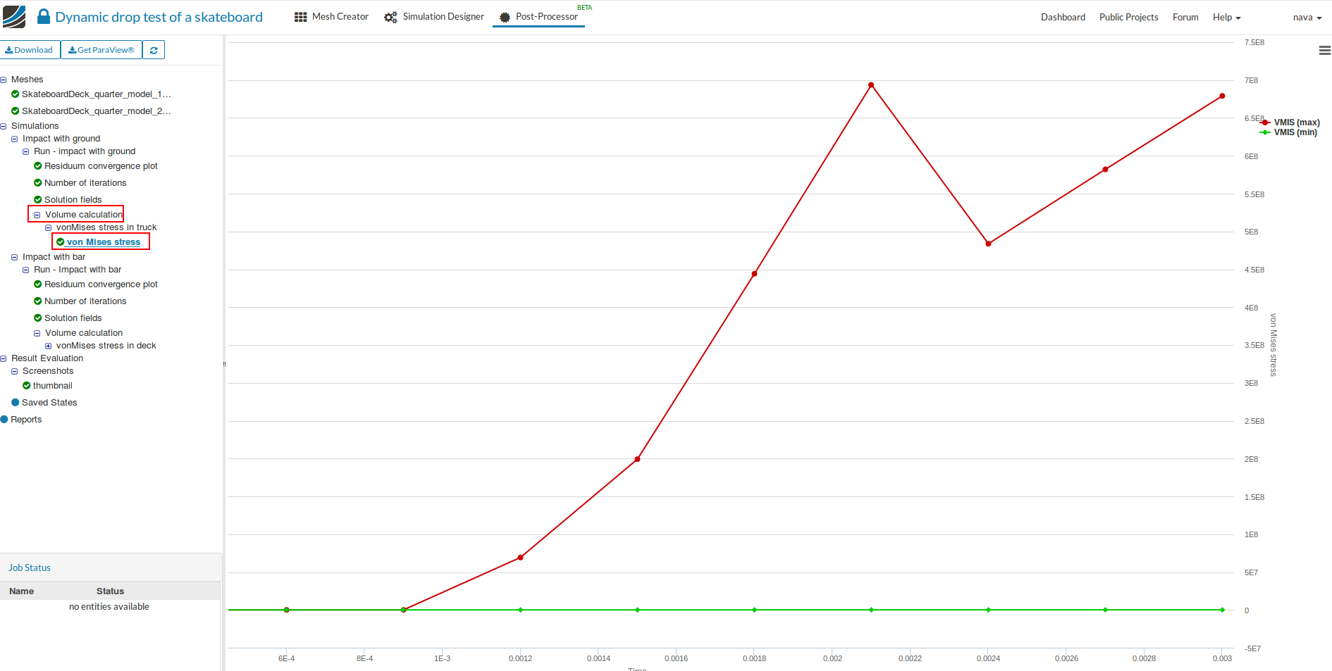
In this simulation we want to observe von Mises stress in volumes - VolumeOnGeoVolumes_2 and VolumeOnGeoVolumes_3.

Add an additional result control item by clicking on Result Control and then New under Volume Calculation.

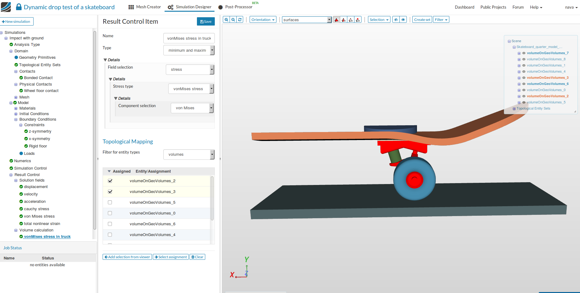
13-result_control1.png1892×950 157 KB
Give a suitable name - vonMises stress in truck. Select stress for Stress type, von Mises for Component Selection , select VolumeOnGeoVolumes_2 and VolumeOnGeoVolumes_3 and finally click Save.

Create New Run

Click on Simulation runs and create a new run. Give the simulation run a suitable name (optional) e.g. Run - impact with ground in this case.

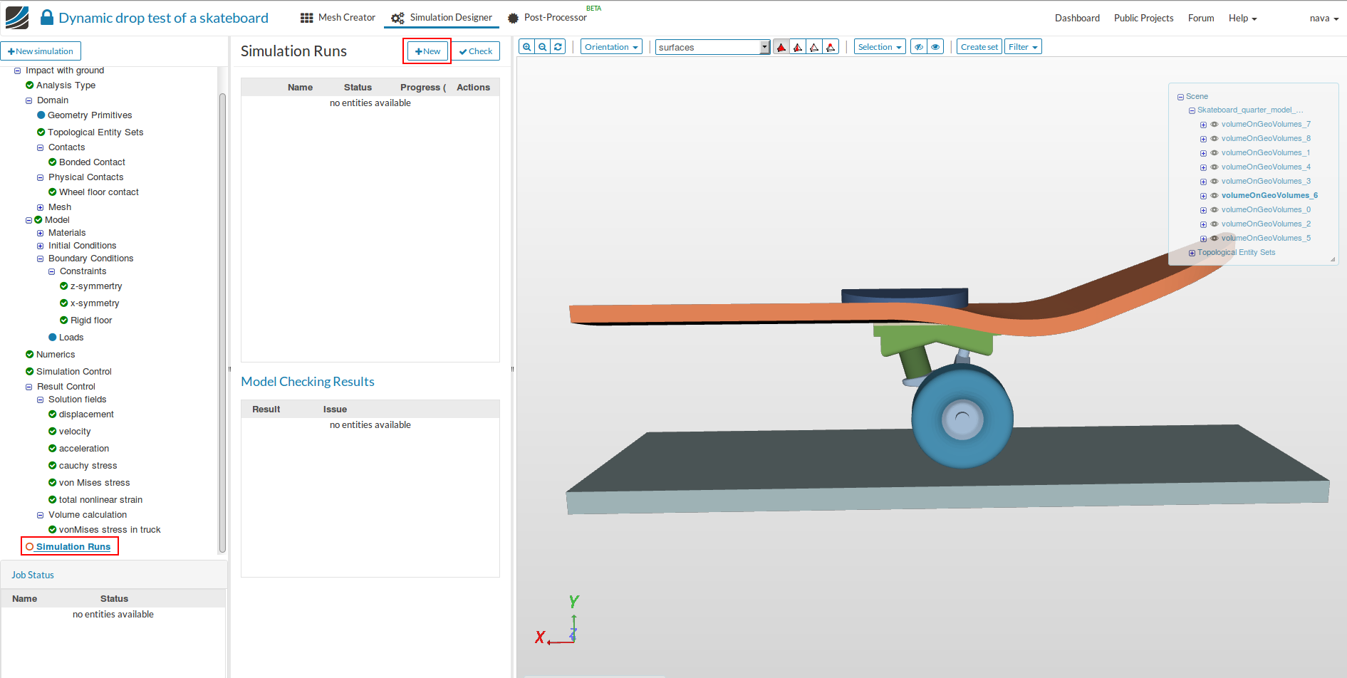
The new run will be created under Simulation Runs. Click Start to run the simulation.

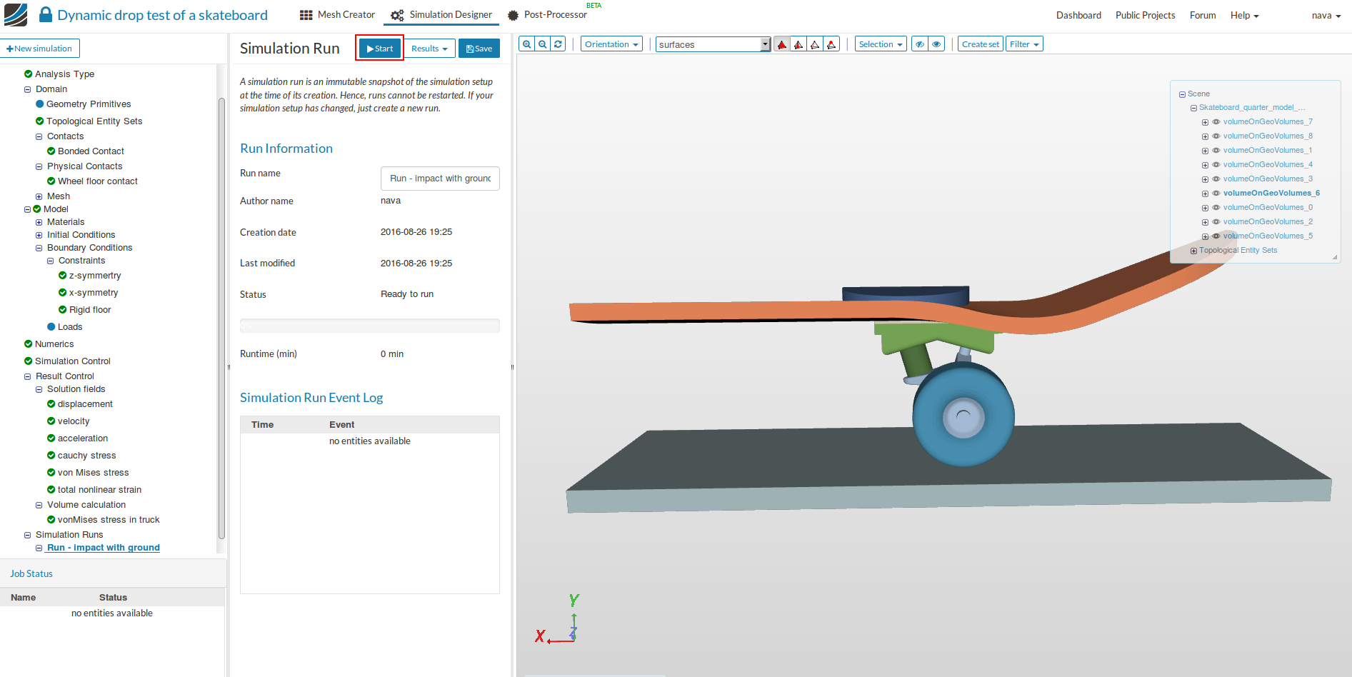
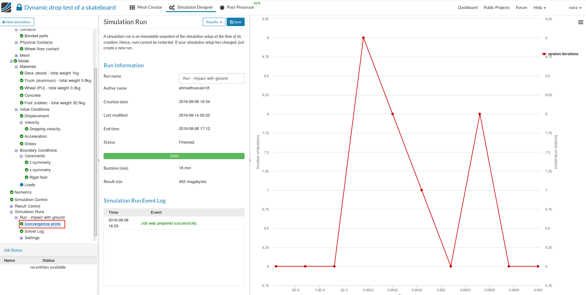
The run will start automatically, will take around 18 min to complete and gives a ‘Finished’ status on completion.
If you want to see the convergence plot, click on Convergence plots under Run - impact with ground. The convergence plot will appear on the right side.

Post-processing

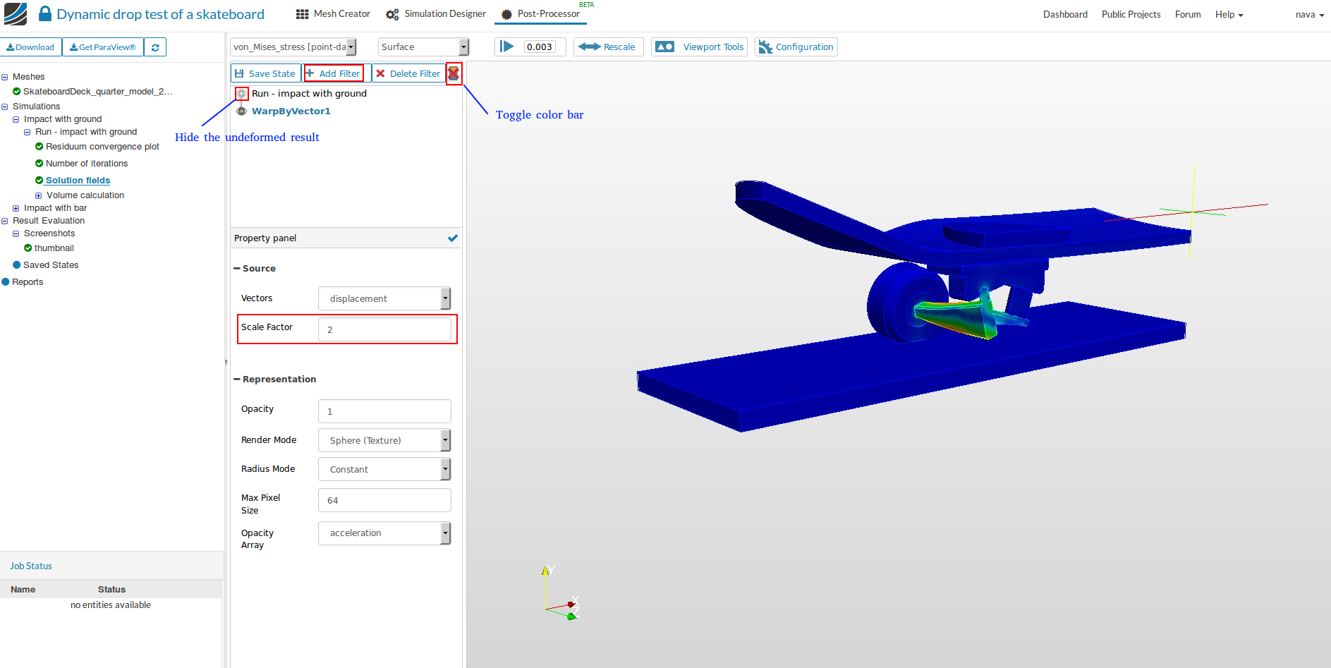
Once the simulation is over, click on Post-processor tab to view the results.
Select Solution fields of the simulation run you want to view results. In this case it is Run - Impact with ground.
To see the deformed geometry, click on Add Filter and then Warp by Vector. You will see a Warp by Vector filter is added under your solution field, and in the result viewer the deformed skateboard will appear with the undeformed shape. You can select Toggle color bar to view the magnitude of the von Mises stress (right side of the Delete Filter button).

The undeformed result can be hidden by clicking on the Eye button at the left of Run - Impact with ground.
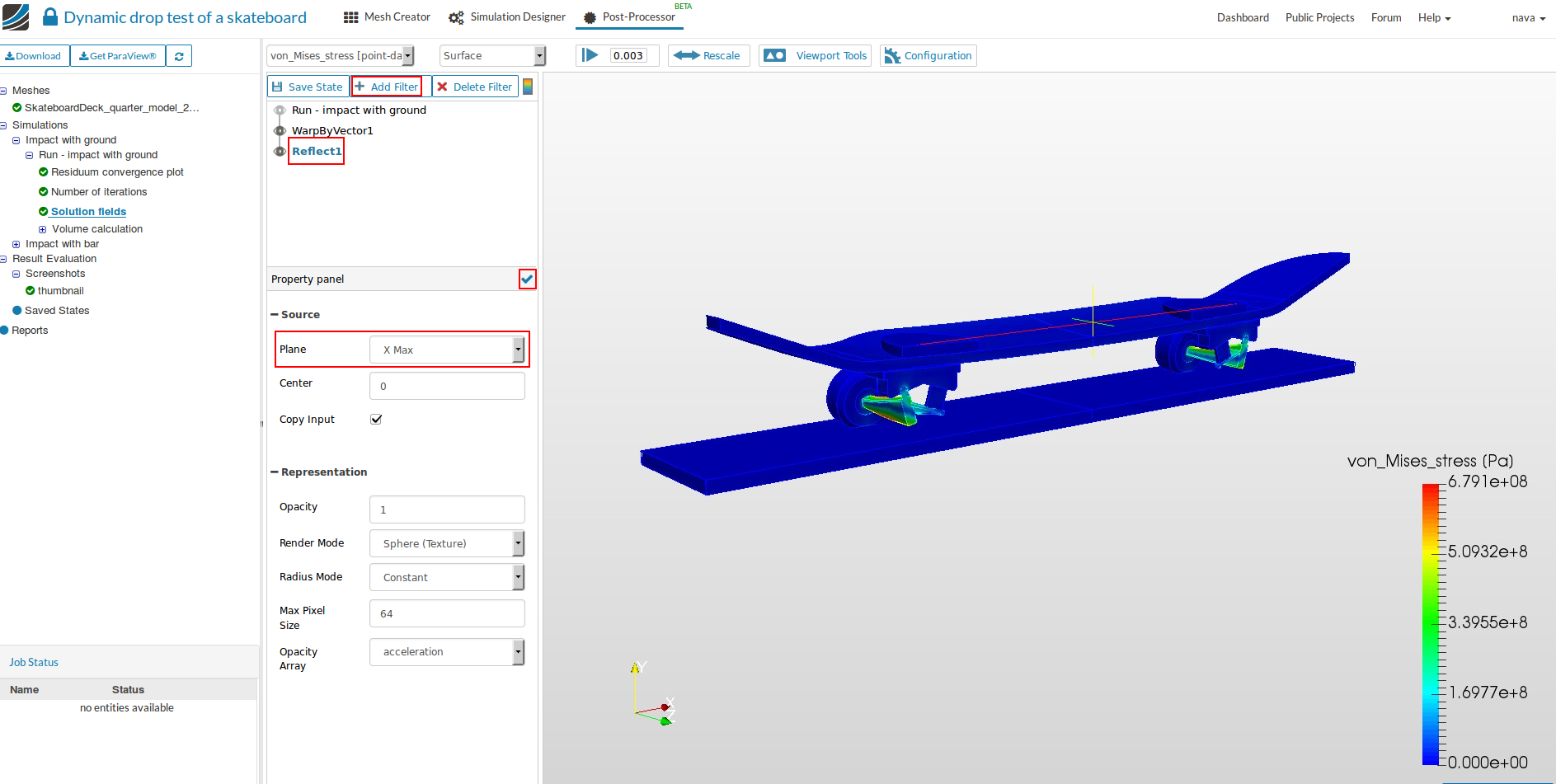
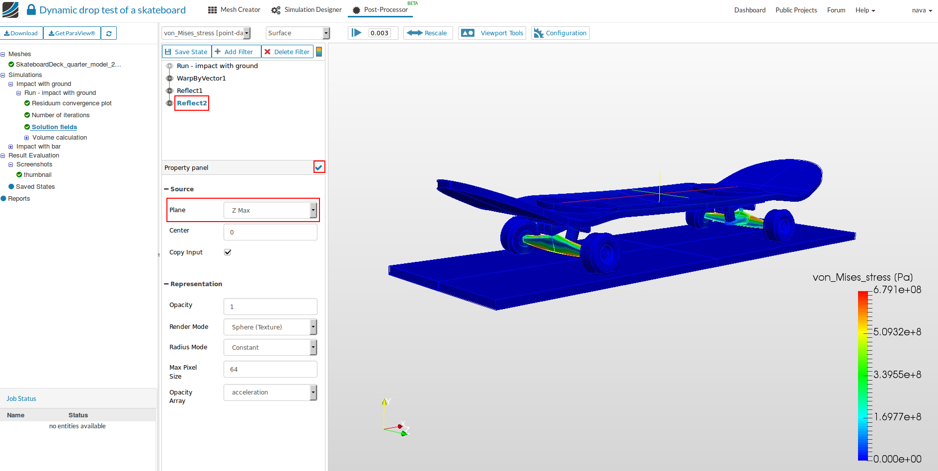
The geometry visible in the post processing window is only a quarter of the whole skate board. So, in order to view the whole geometry we have reflect it along positive X and Z direction.
Click on Add Filter and then Reflect. Choose X Max for ‘Plane’ and then click on tick mark to apply changes.

8-pp2_reflect_x.png1887×951 317 KB
Repeat the same step for reflecting it along positive Z direction. Now you can see the stresses at the end time step for the complete geometry.

In order to see the animation, click the play button which will animate all the saved 20 steps.

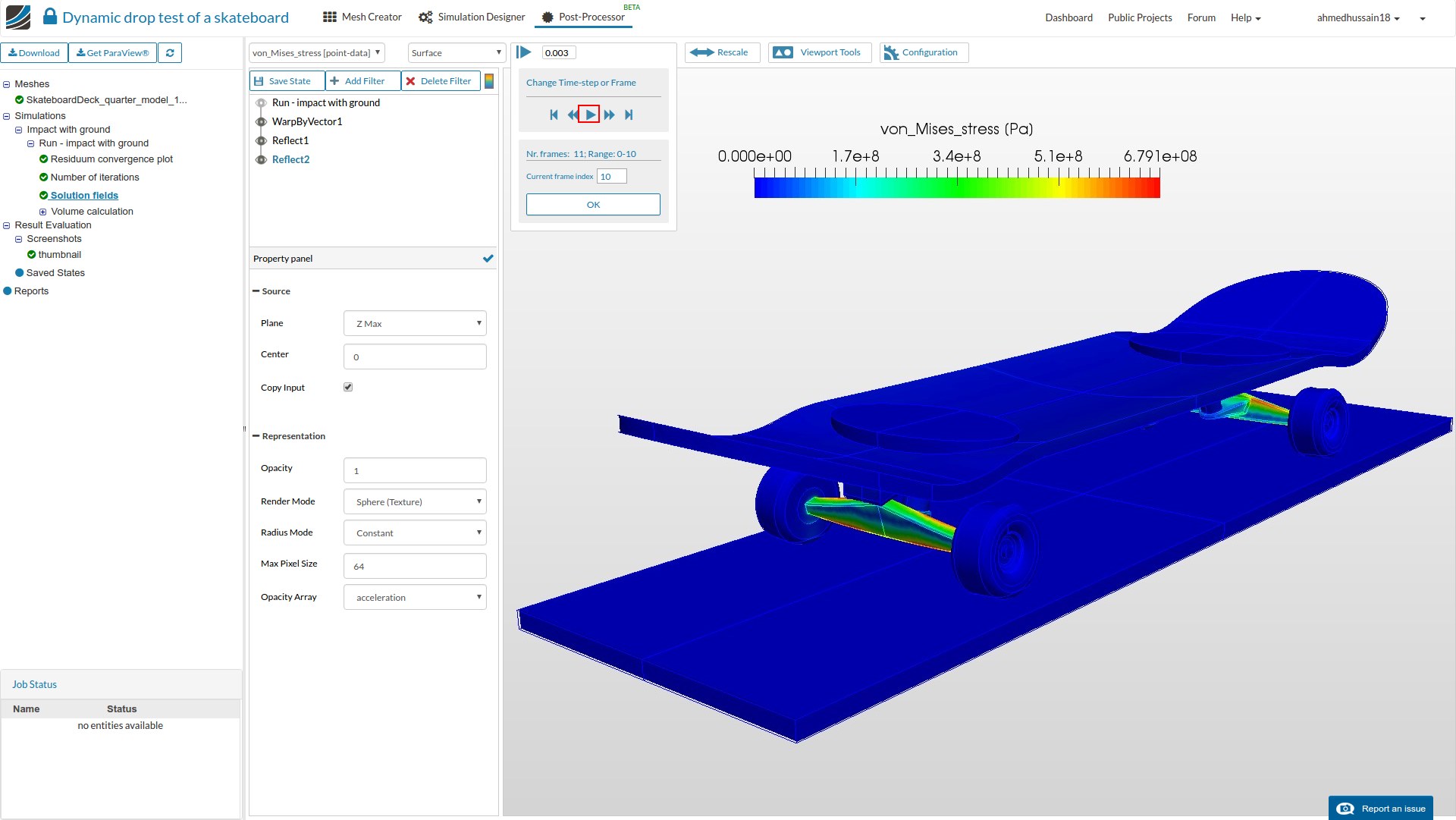
The animation will look something like this:

You can see the time variation of maximum von Mises stress in the truck of the skateboard by clicking on von Mises stress under Volume Calculation.