Our aim is to analyse snap-fitting buckles. In this project we will give a displacement of 0.02 mm to the male end of the buckle keeping the female end fixed. The displacement is chosen such that male end completely snap fits and hits the support shoulder. Since the geometry and loads are symmetric about the centre plane, only half model is used for the analysis to save time.
Step-by-Step
Import the project by clicking the link below. (Crtl + Click to open in a new tab).
https://www.simscale.com/workbench?publiclink=3ffdd729-bd71-41c0-afd4-c3bdd8cfafb1
Once the project is imported, the workbench is automatically opened. Then follow the steps below for setting up the simulation.
Meshing
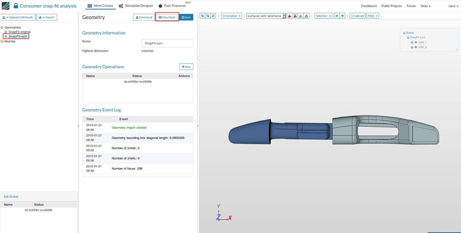
- In the Mesh Creator tab, click on the geometry SnapFit-sym. You will see a half model of the buckle in your viewer.
- Then, click on New Mesh button in the options panel.
-
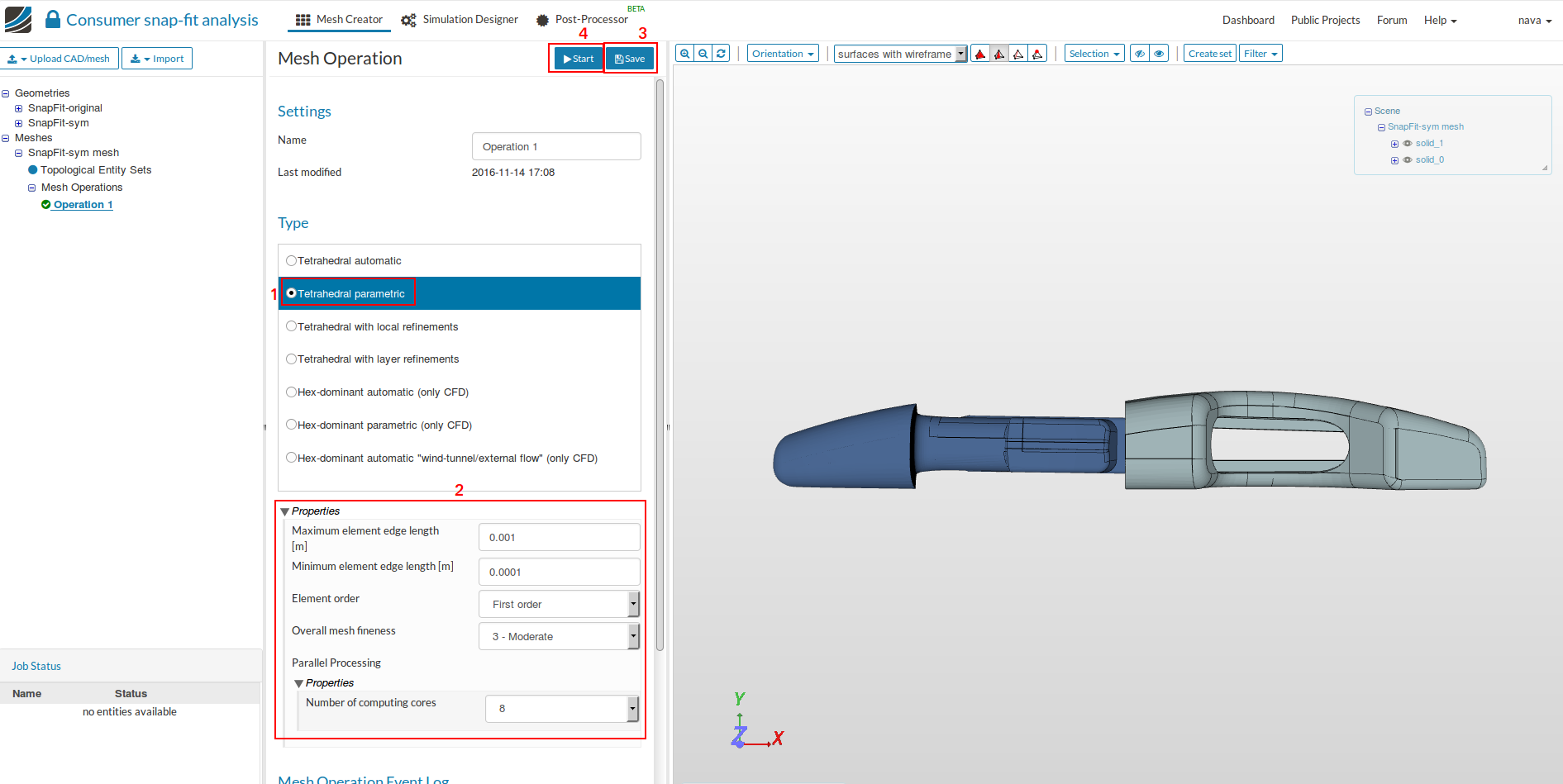
Select Tetrahedral parametric [1] for the mesh and use the following parameters [2] - 0.001 and 0.0001 as maximum and minimum mesh edge length respectively, First order for the desired mesh order, 3-Moderate fineness and 8_ computing cores_. Also, set the NETGEN3D to be True.
-
Save [3] the settings.
-
Click on Start [4] button to start the meshing operation. The meshing job will start in a few moments and all computation is done via cloud computing.
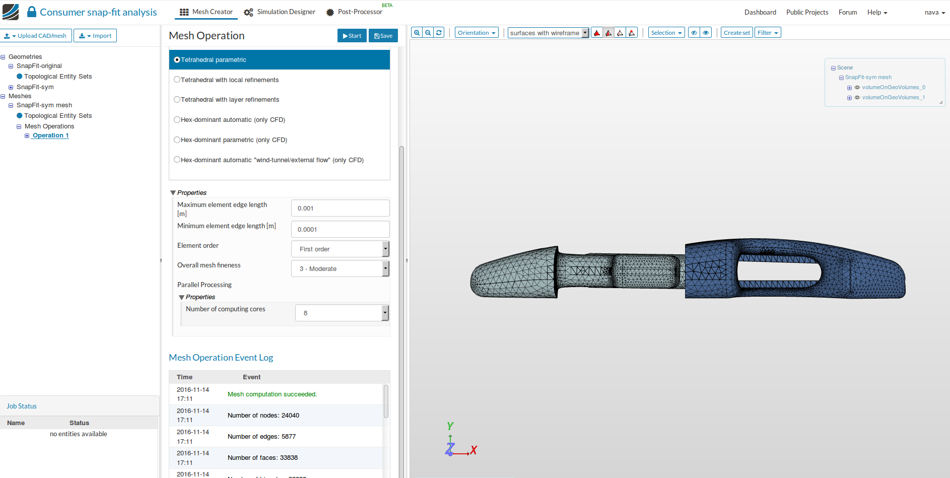
- The mesh operation takes about 5 min to complete and gives a Finished status in the lower left corner once it is over. The meshed geometry can be seen in the viewer.
Simulation Setup
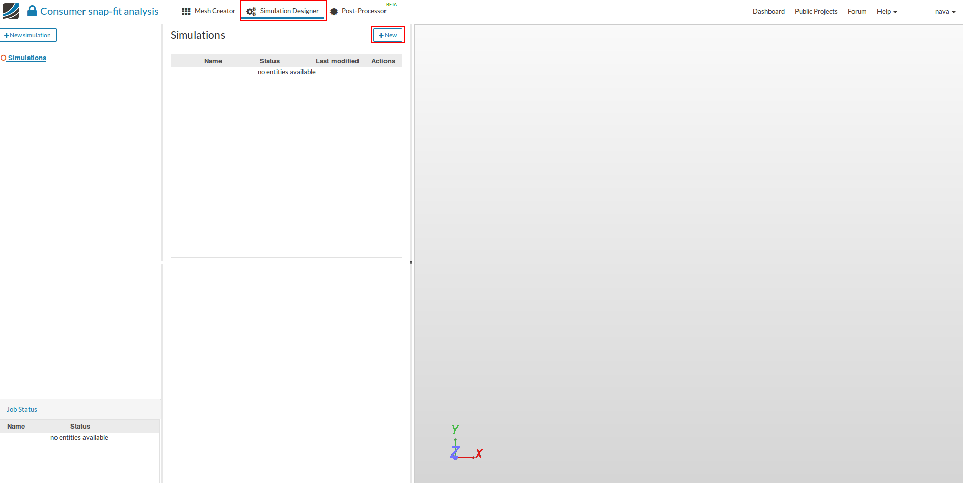
- For setting up the simulation, switch to the Simulation Designer tab and select New button.
-
A create new project window will pop-up. Give a suitable project name (optional) and click Create.
-
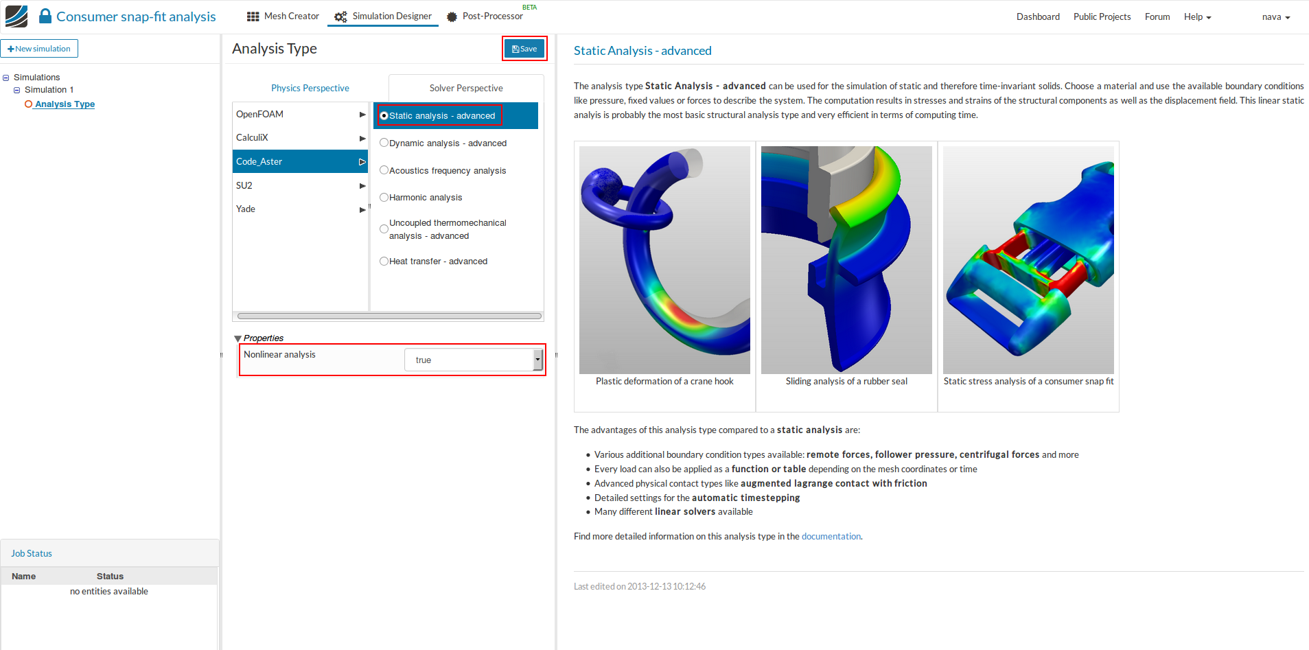
Since our simulation involves physical contact, select the analysis type Static analysis - advanced under Code_Aster (Solver Perspective), change Nonlinear analysis to true and click Save.
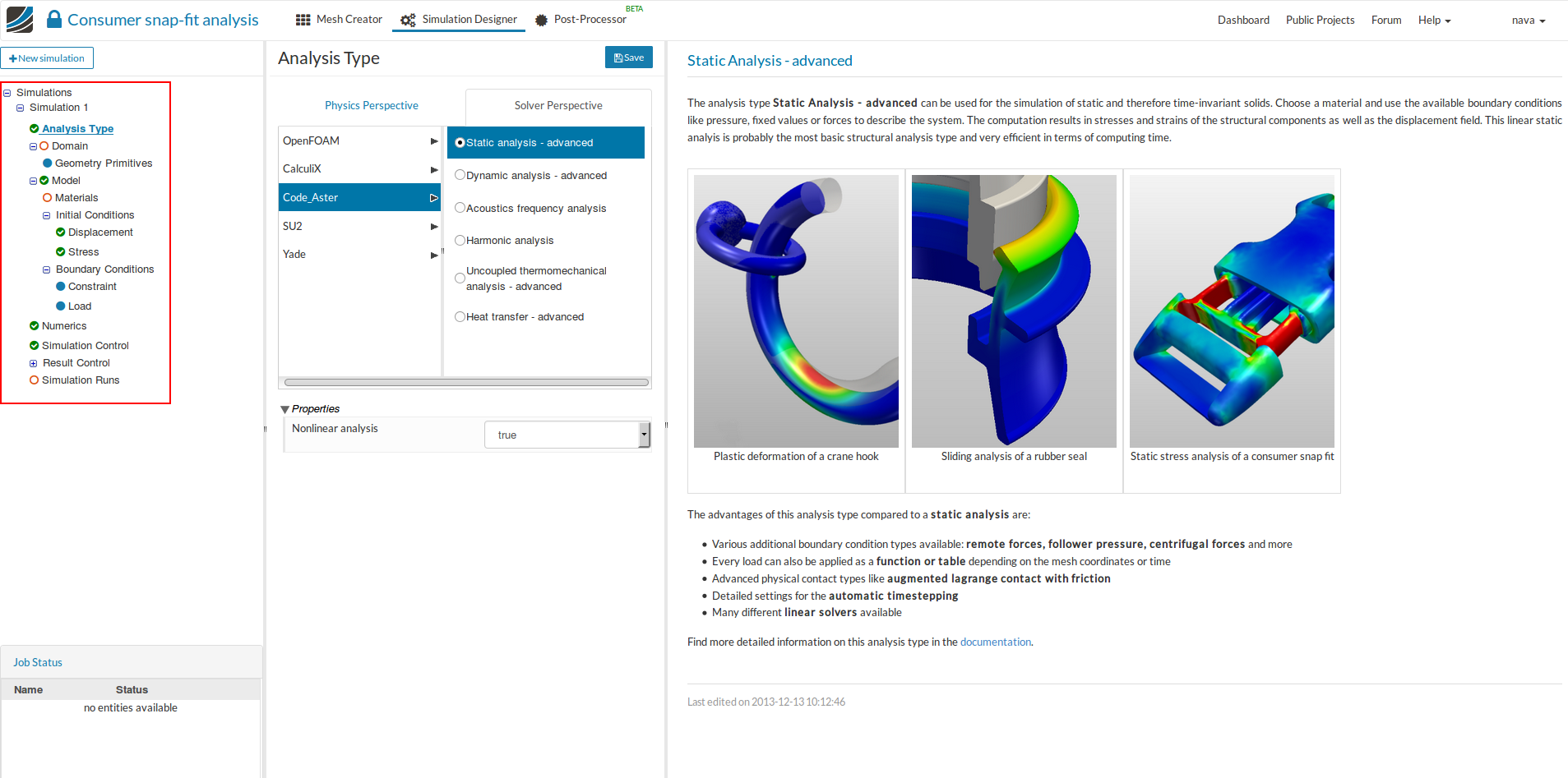
- After saving, the simulation tree now looks as shown below. Here the tree entries in red must be completed.
Domain selection
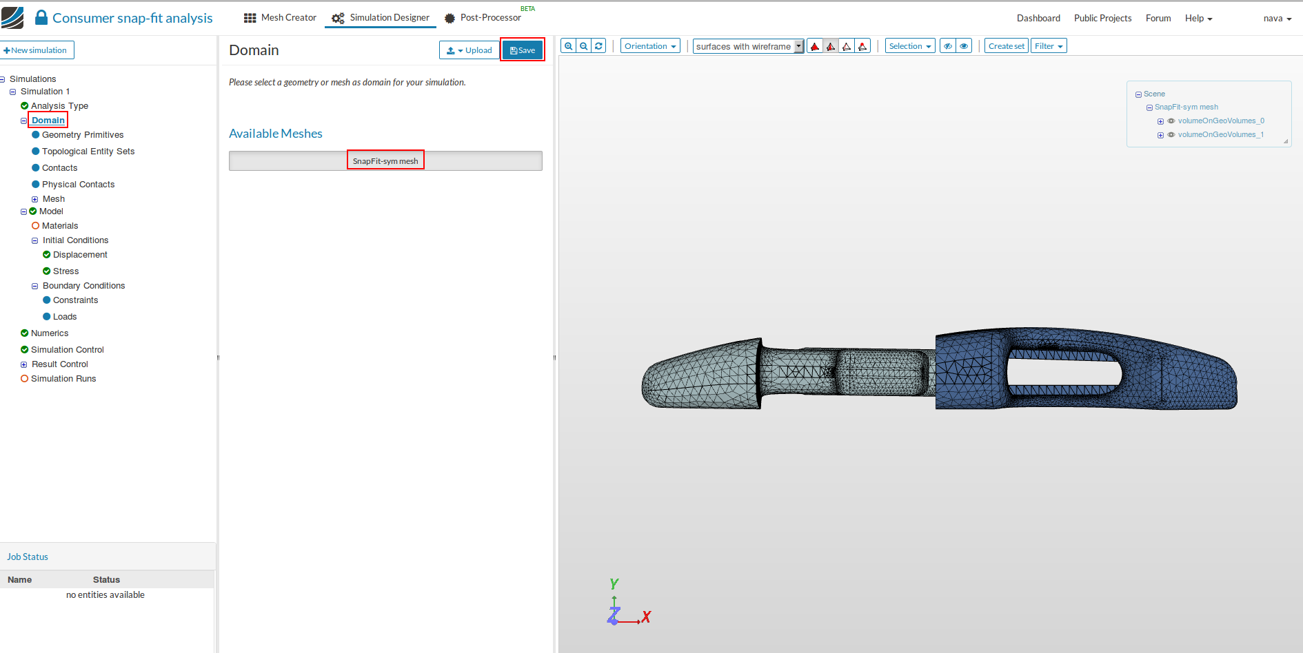
- Click on Domain from the tree and select the mesh created from the previous task. Click on the Save button. The mesh will be automatically loaded in the viewer.
Create Topological Entity Sets
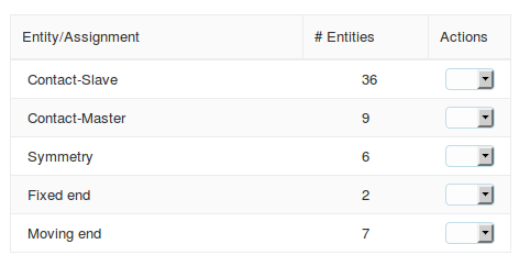
- In this tutorial, we need 5 topology entity sets for specifying the boundary conditions and physical contacts.
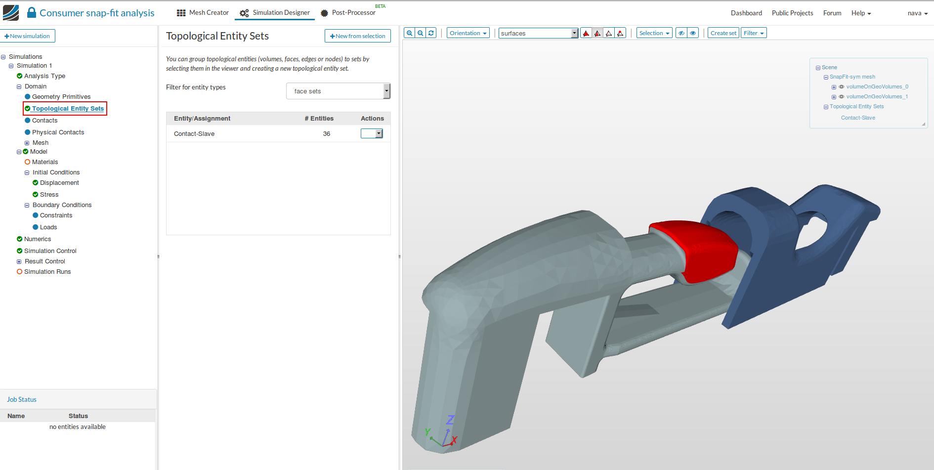
- Click on the tree entry Topological Entity Sets.
Contact-Slave:
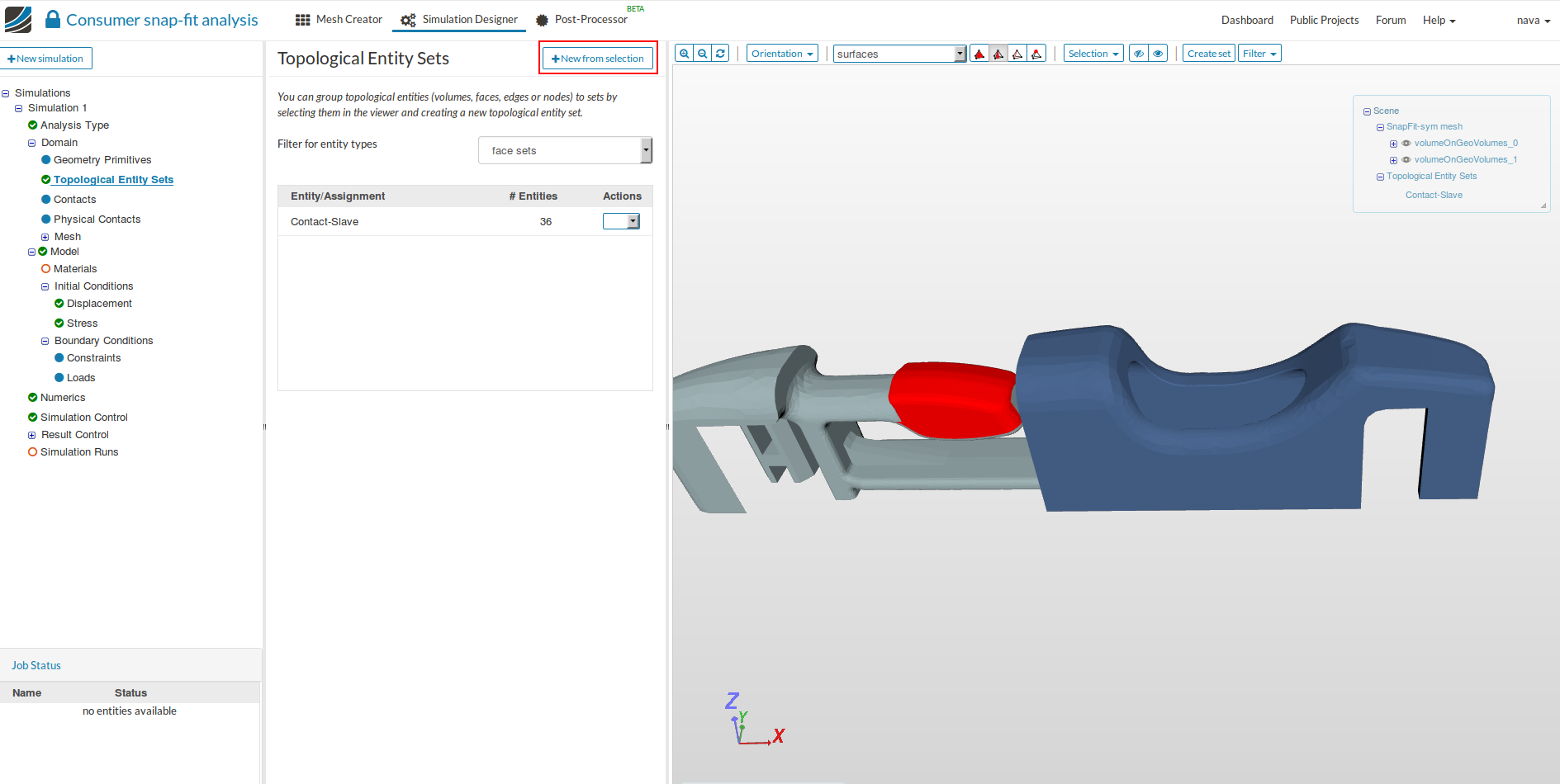
- To create the first set, select the shown surfaces and click on the New from selection button to create a set named Contact-Slave. Here we are creating the contact surfaces which will serve as a slave entity in the physical contact.
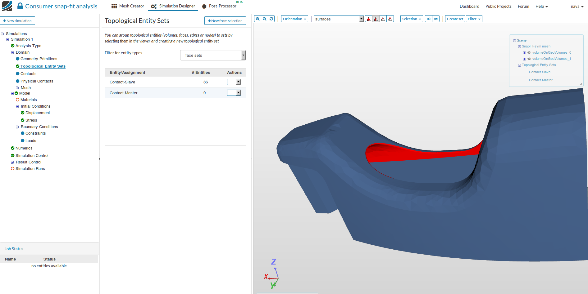
Contact-Master:
- Follow the same step as above for creating the second topological set with a different set of faces as shown in the figure below.Here we are creating the contact surface which will serve as a master entity in the physical contact.
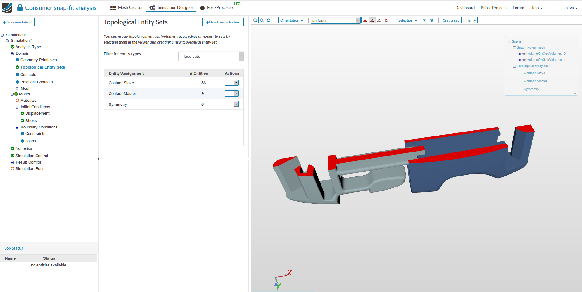
Symmetry:
- Follow the same step as above for creating the third topological set with a different set of faces as shown in the figure below. Here, we are making a set of faces that are cut by the plane of symmetry.
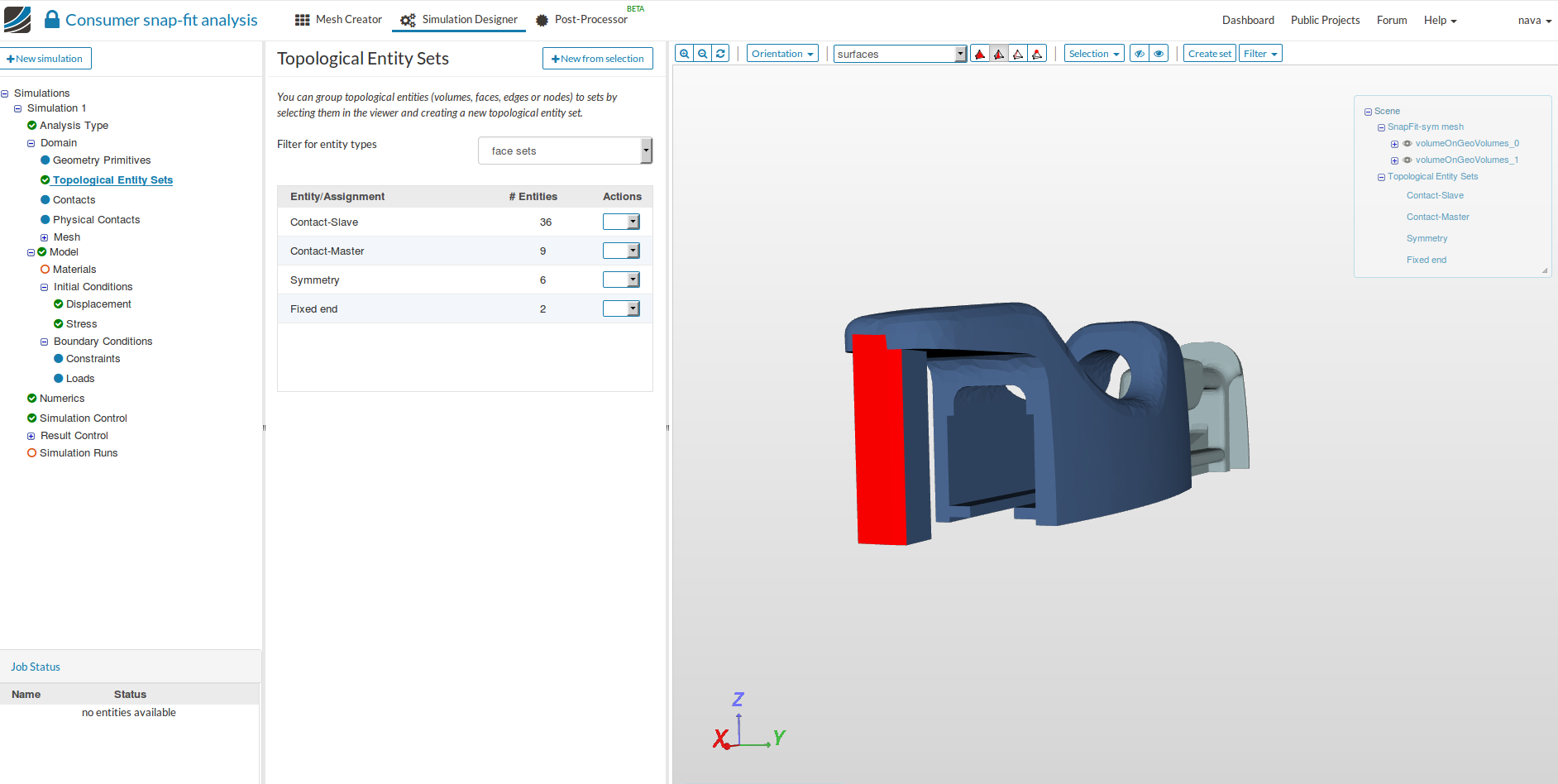
Fixed end:
- Follow the same step as above for creating the fourth topological set as shown in the figure below. Here, we are making a set of faces in the female end where the displacement will be set to zero.
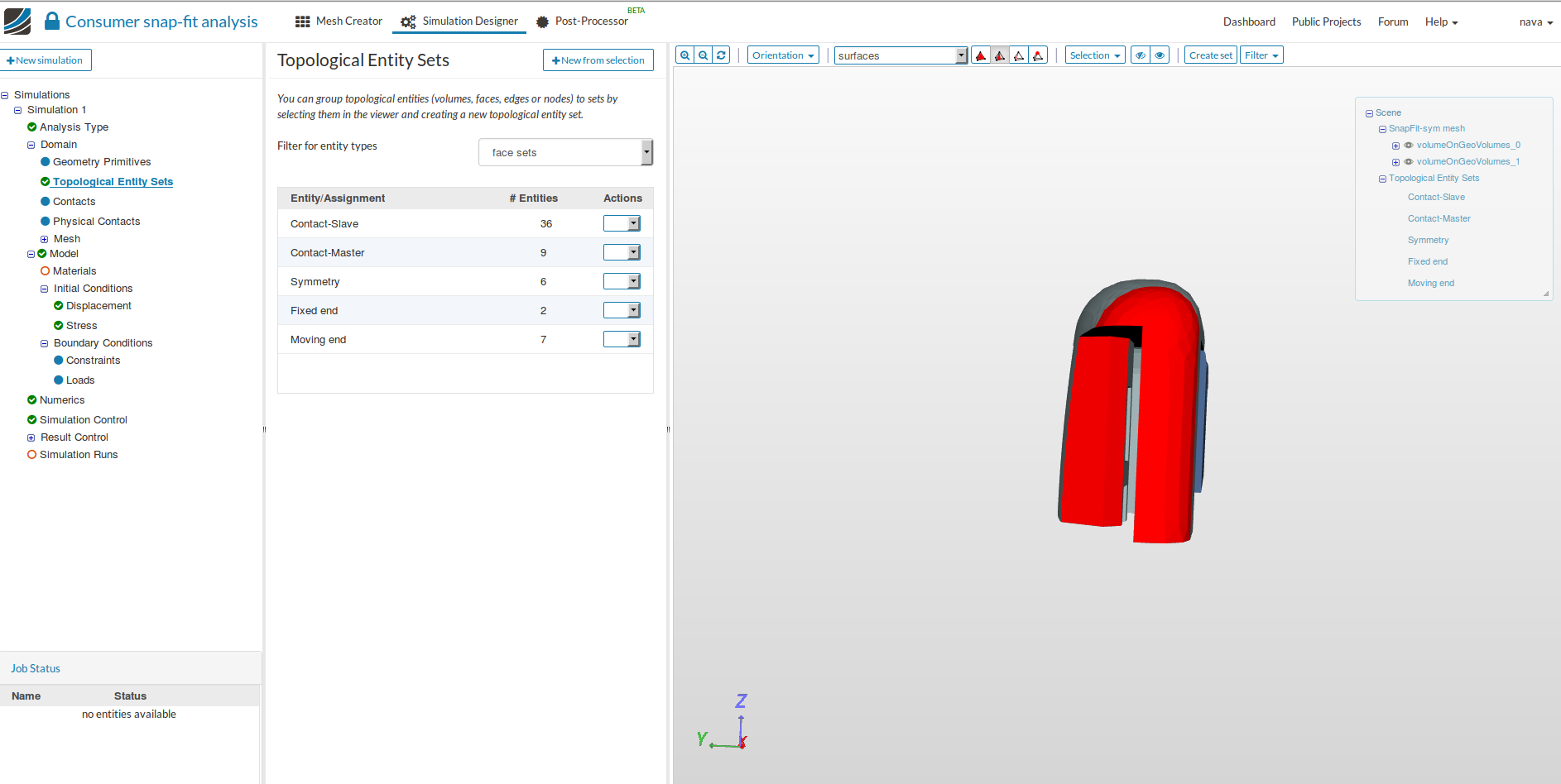
Moving-end:
- Follow the same step as above for creating the fifth topological set as shown in the figure below. Here, we are making a set of faces in the male end where the a displacement will be applied.
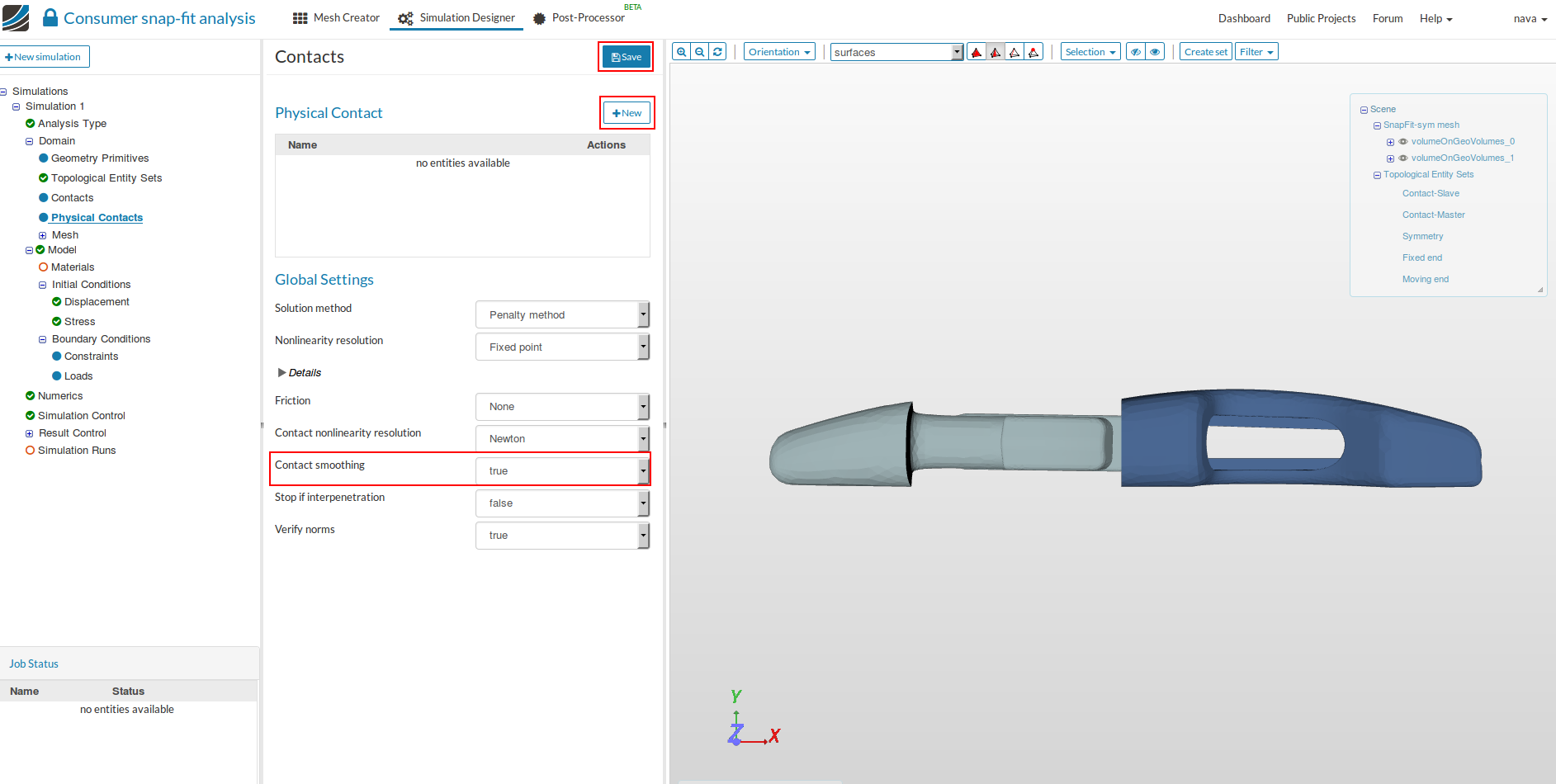
Physical Contacts
In this section we will define the physical contact between the two bodies. We are using penalty method for modelling the contact.
-
Select Physical Contacts and then click on New. The Penalty method is available as default. Change the Contact smoothening to true and Save the settings. This is required for convergence and stability of the solution when there is a curved contact zone with first order elements.
-
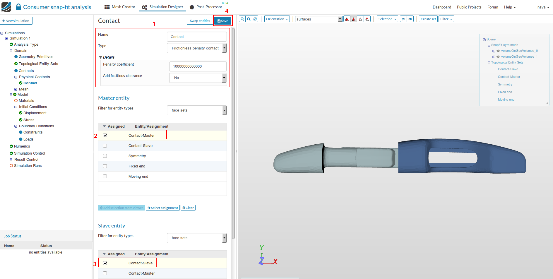
Click on New to create a new contact.
- Change the Name to Seat with rigid contact (optional) and give a very high value of
Penalty factor ( 1e13) [1]. - Here, we are not considering friction at the contact, therefore choose Frictionless penalty contact as Type [1].
- Select Rigid-seat contact as a Master entity [2] and Seal-rigid contact [3] as Slave entity and then click Save [4].
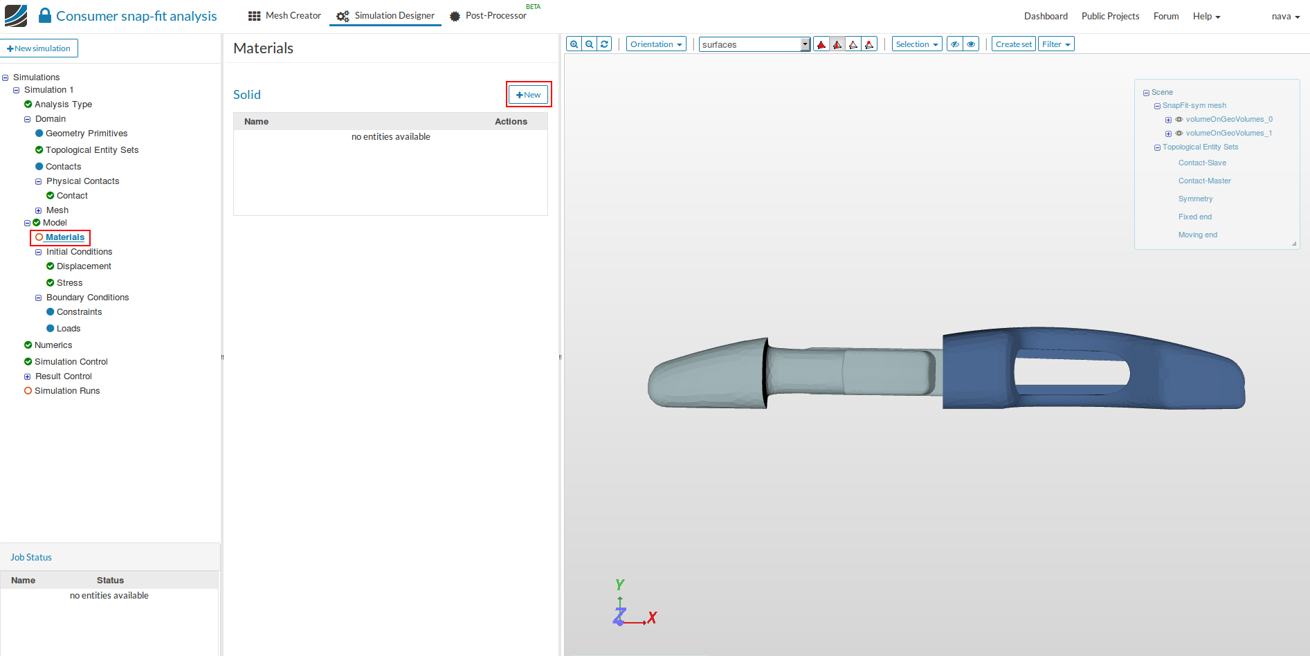
Select Solid Material
- Now we will define material for our two bodies. Select Material from the sub-tree and click New.
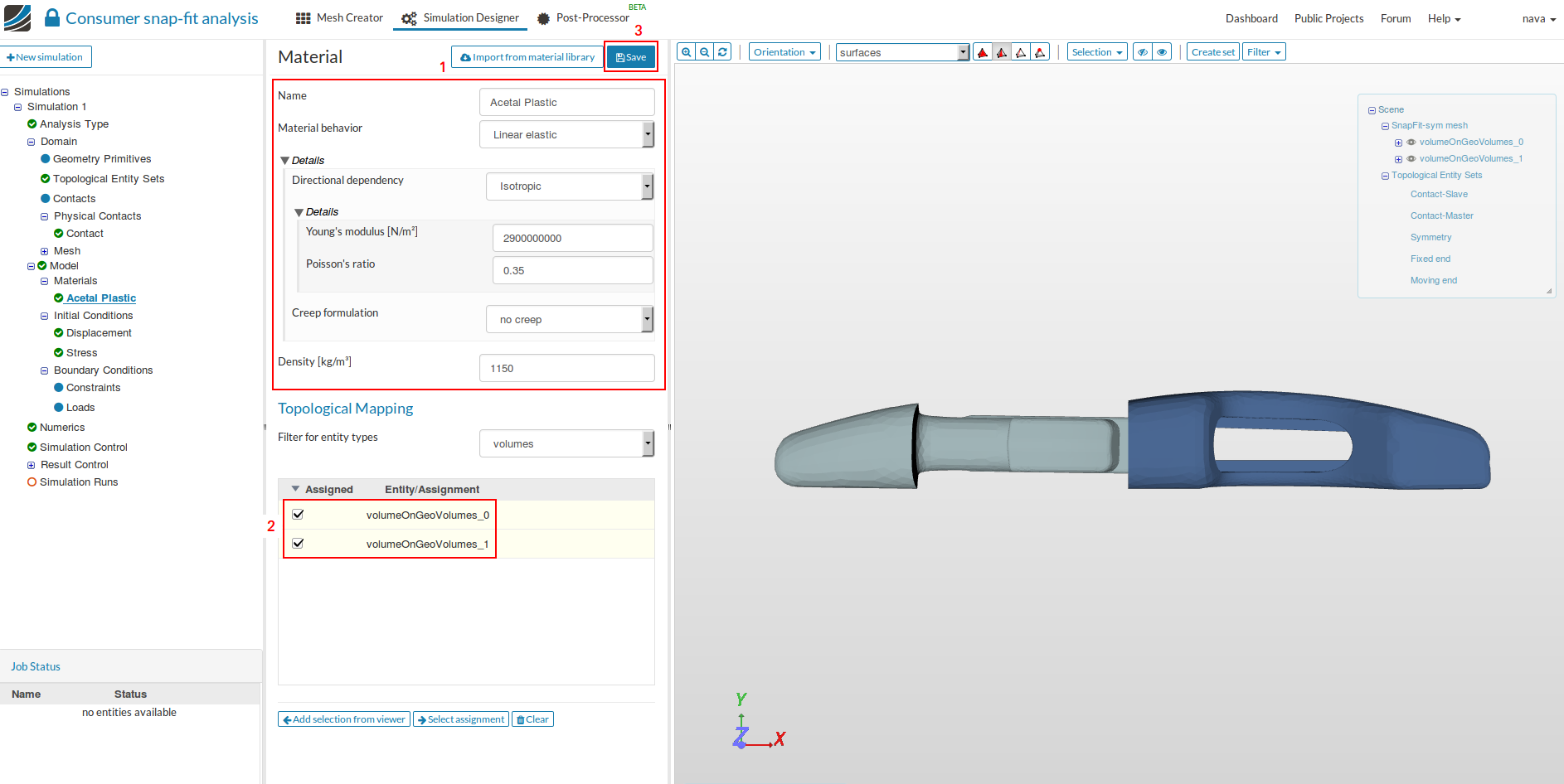
- Change the following parameters [1]:
- Name: Acetal Plastic (optional)
- Young’s modulus [N/m2]: 2900000000
- Poisson’s ratio: 0.35
- Select volumeOnGeoVolumes1 (rigid body) [2] to add the volume to which steel is assigned and then Save [3].
Boundary Conditions
In this section we will define the fixation of the female end, symmetry boundary conditions along the symmetry plane and displacement of the male end.
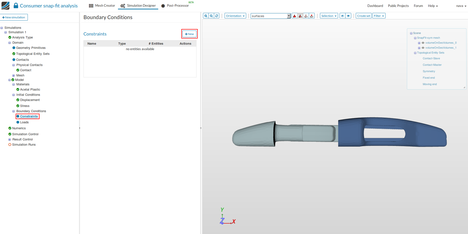
- Let’s first define symmetry. Select Constraint in the tree and click New.
-
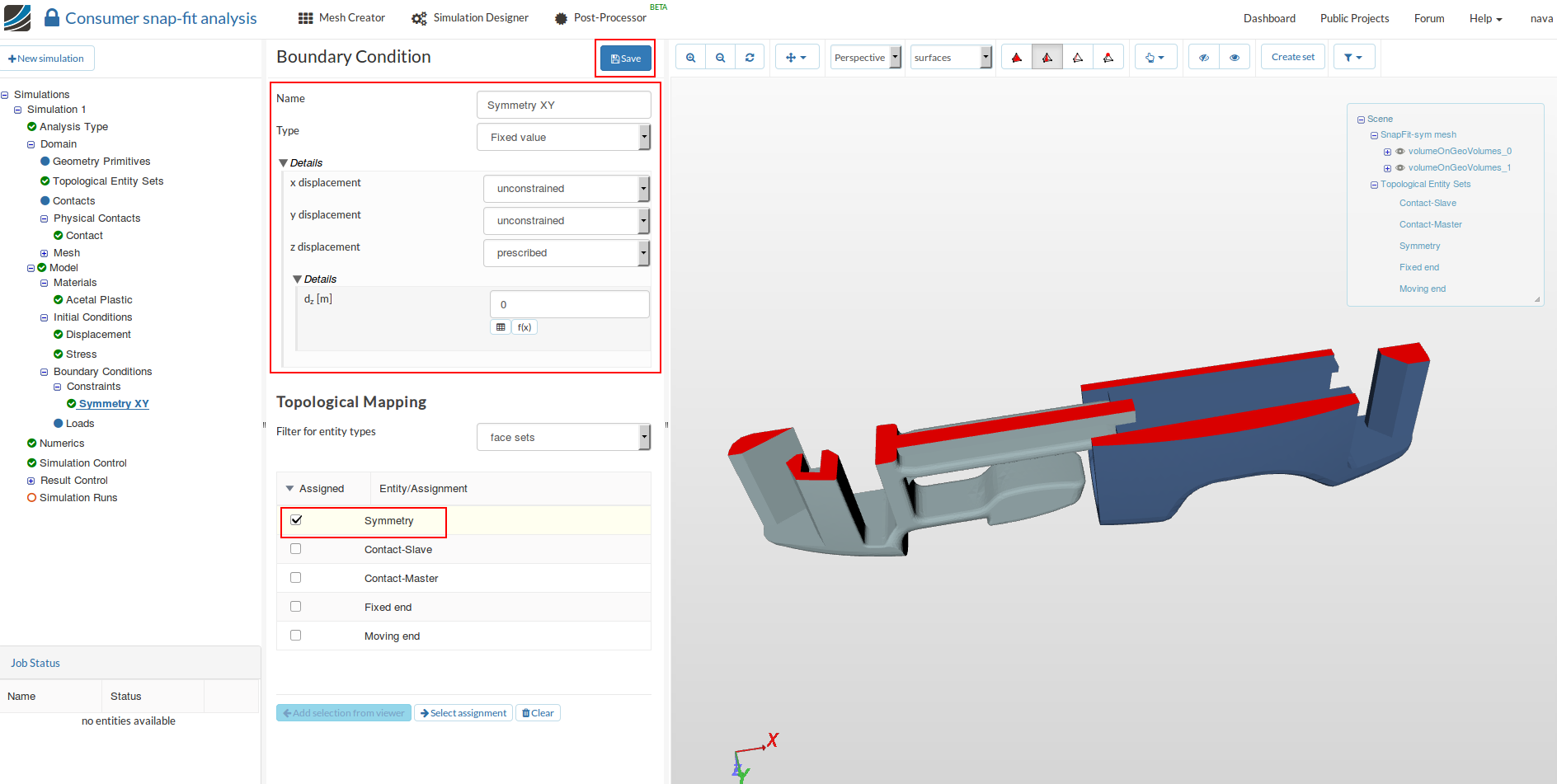
Rename the Boundary condition to Symmetry XY (optional). Choose the Type Fixed value. Set the value for z displacement to 0 and select unconstrained for x and y displacement.
-
Finally Save the settings.
-
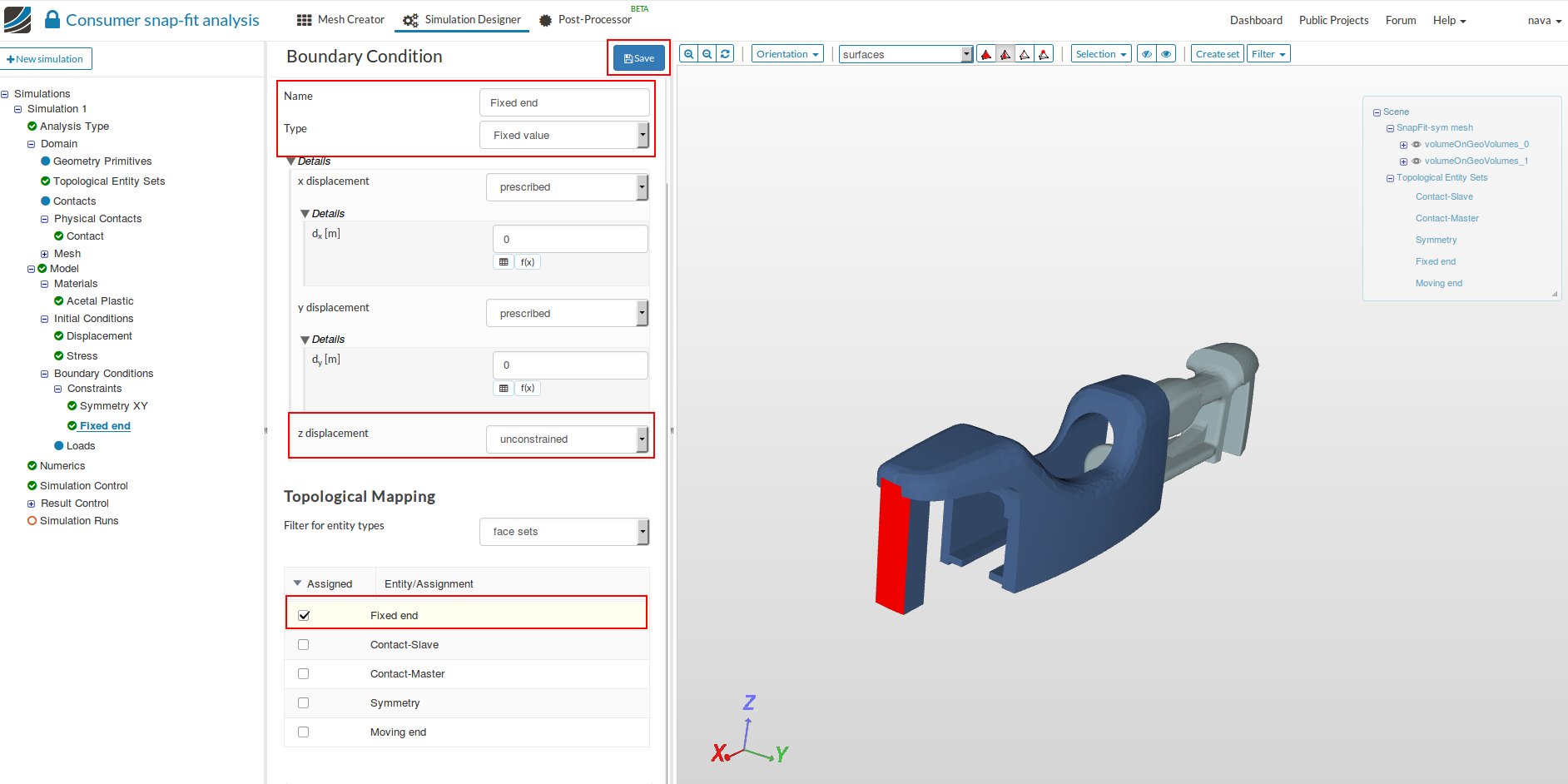
For defining the fixation, select Constraint in the tree and click New.
-
Rename the Boundary condition to Fixed (optional). Choose the Type Fixed value and choose unconstrained for z displacement. The x and y displacement should be 0.
-
Under Topological Mapping, change Filter for entity types to face sets and select Fixed end. Then click Save.
-
For defining the displacement , select Constraint in the tree and click New.
-
Rename the Boundary condition to Moving end (optional). Choose the Type Fixed. Choose unconstrained for z displacement and 0 for the y displacement . For the x displacement, specify it as a function by clicking on ‘function button’ and give 0.02*t in the Formula.
-
Under Topological Mapping, change Filter for entity types to face sets and select Moving end. Then click Save.

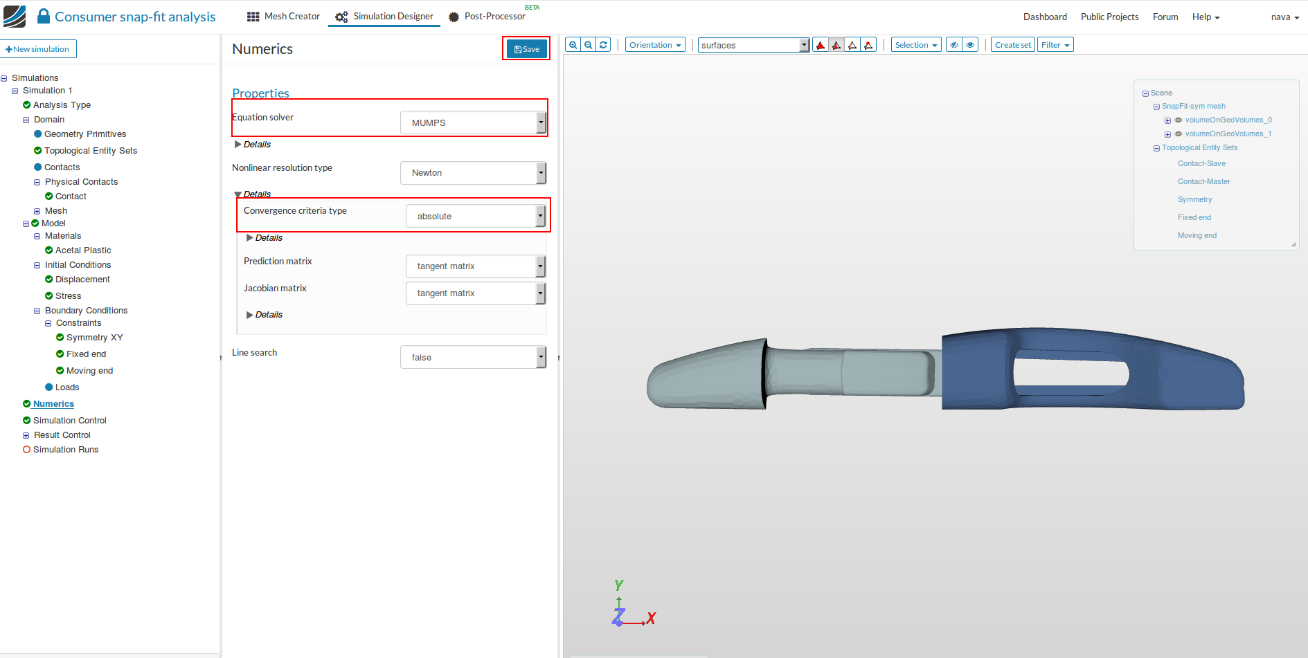
Numerics
Here we specify the type of solver to used. For this simulation we use MUMPS as equation solver. Also, select the Convergence criteria type to Absolute, since the load is given in terms of displacement and not load. And finally, Save the settings.
Simulation Control
- Click on Simulation control and change Initial time step length [s] to 0.025 under details of Timestep definition, Number of computing cores to 8, under details Number of cores used for the computation to 4 and Maximum runtime [s] to 20000.

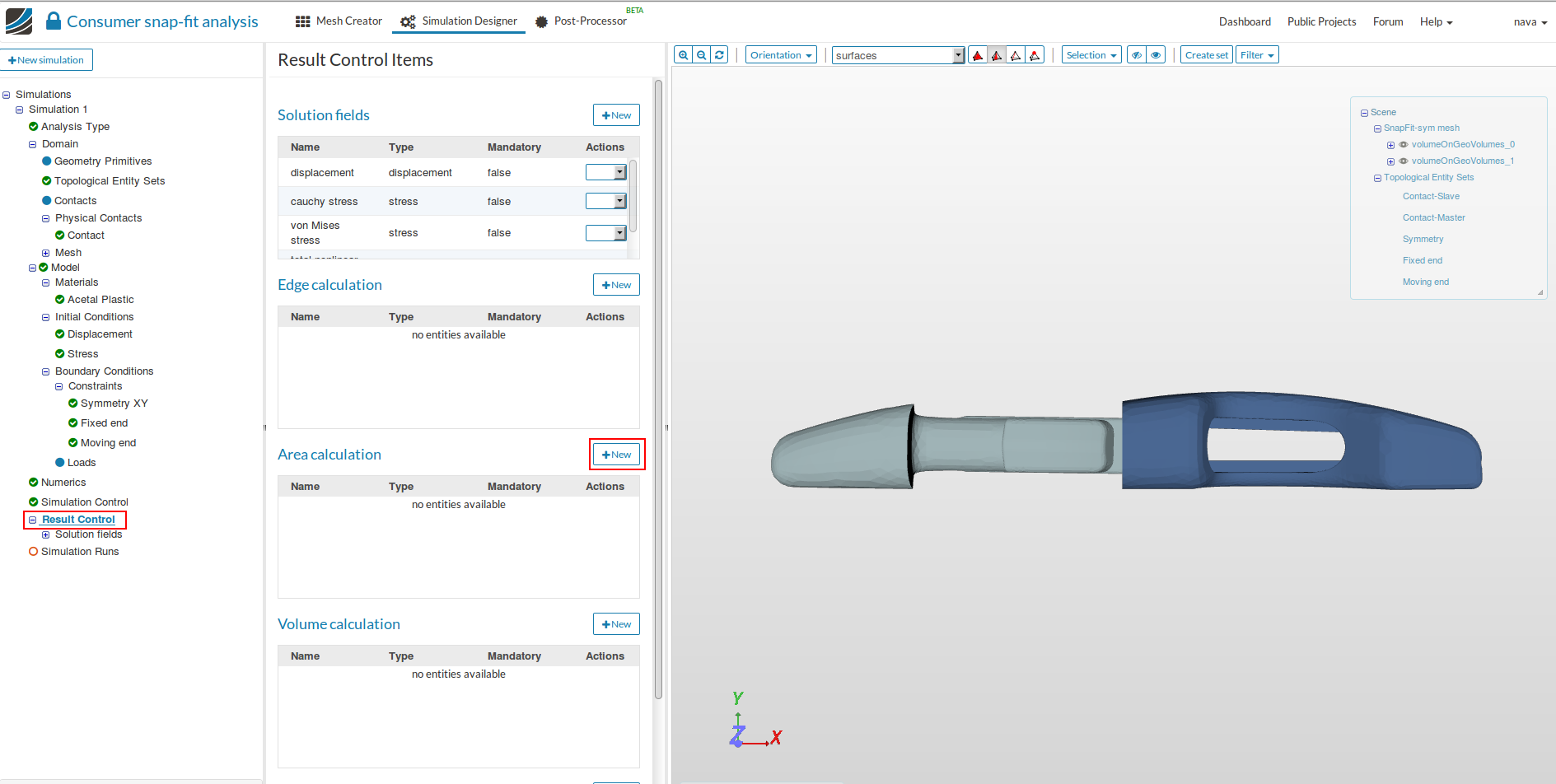
Result Control
In this simulation we want to observe the displacement of snapping teeth and also variation the forces at fixed and moving end with respect to the pseudo time, which is proportional to the applied displacement.
- First, we will create a displacement result control item. Click on Result control and then click on New button associated with Area calculation.
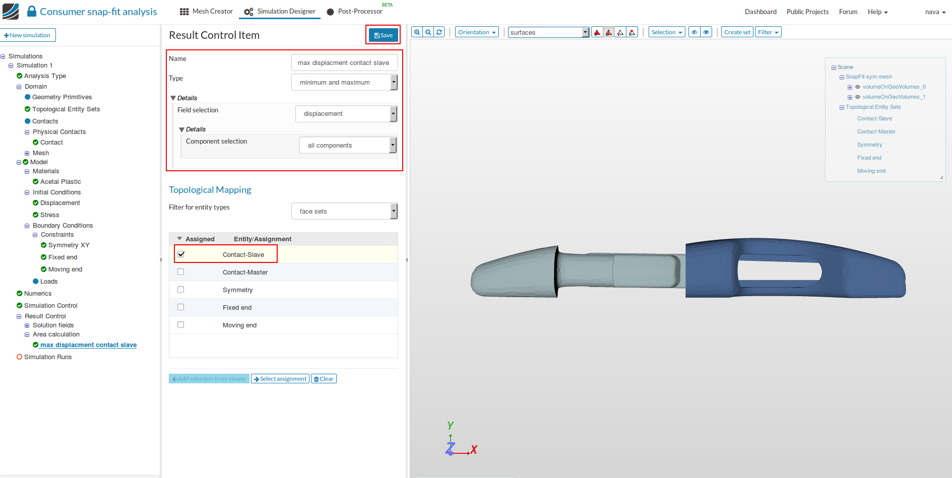
- Specify a suitable name for the result control item e.g. max displacement contact slave (optional), choose minimum and maximum under Type. Under Details choose displacement for Field selection and select all components for Component selection. Finally assign Contact Slave under Topological Mapping and Save.
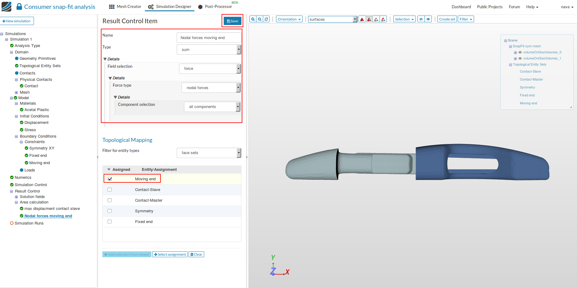
Next we will create result control item which will give variation of force required to move the moving part with time/displacement.
- For this, create a new result control item (Area Calculation) by following the procedure as above. Give a suitable name e.g. Nodal forces moving end (optional) and select sum for Type. Under the Details choose force for Field selection and select all components for Component selection. Finally select Moving end under Topological Mapping and Save.
- Next for the reaction forces at the fixed end, follow the same procedure as above, except choose Fixed end under Topological Maping and change the name to Nodal forces fixed end.

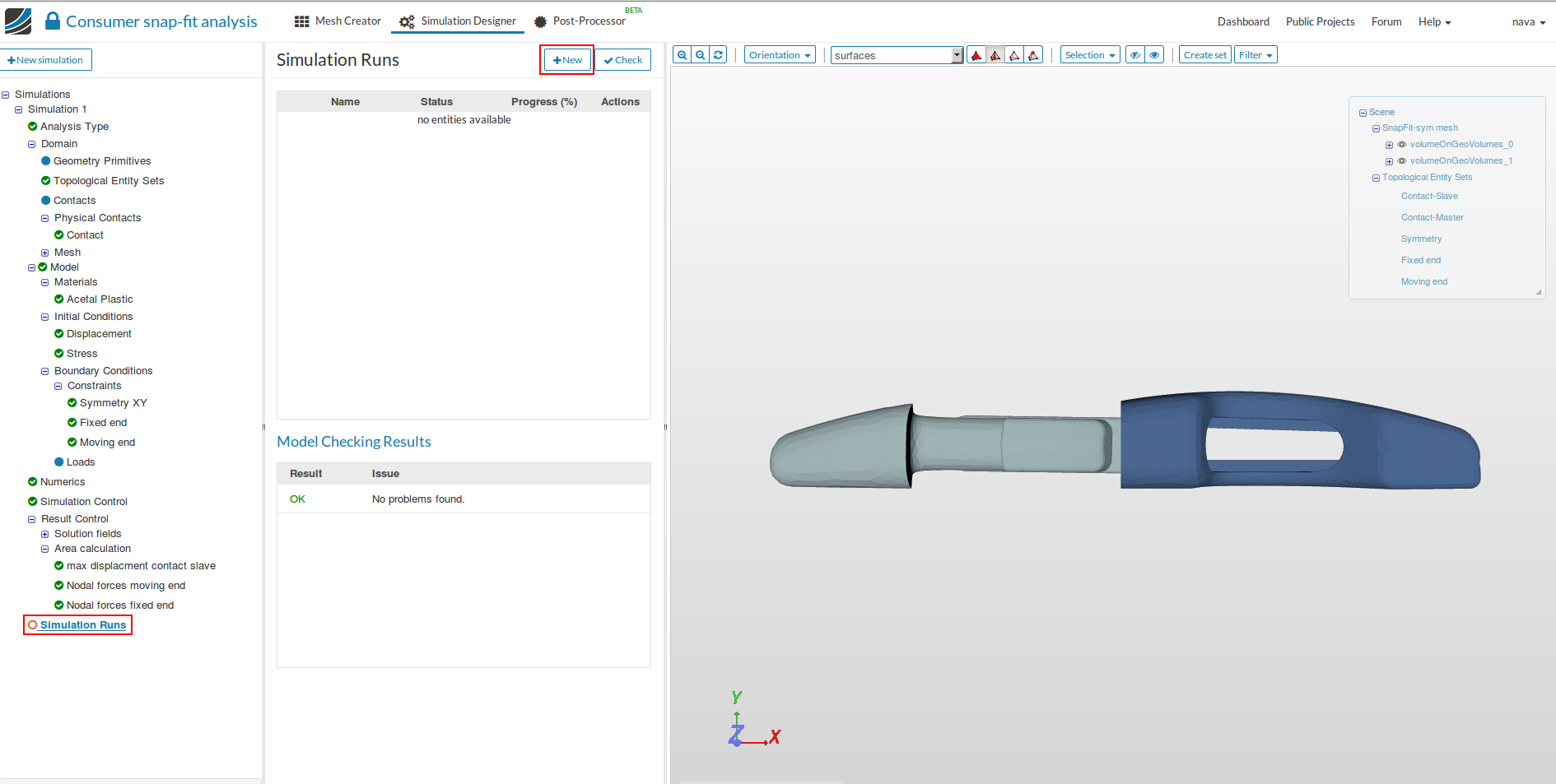
Simulation Run
- Click on Simulation runs and then on New to create a new simulation
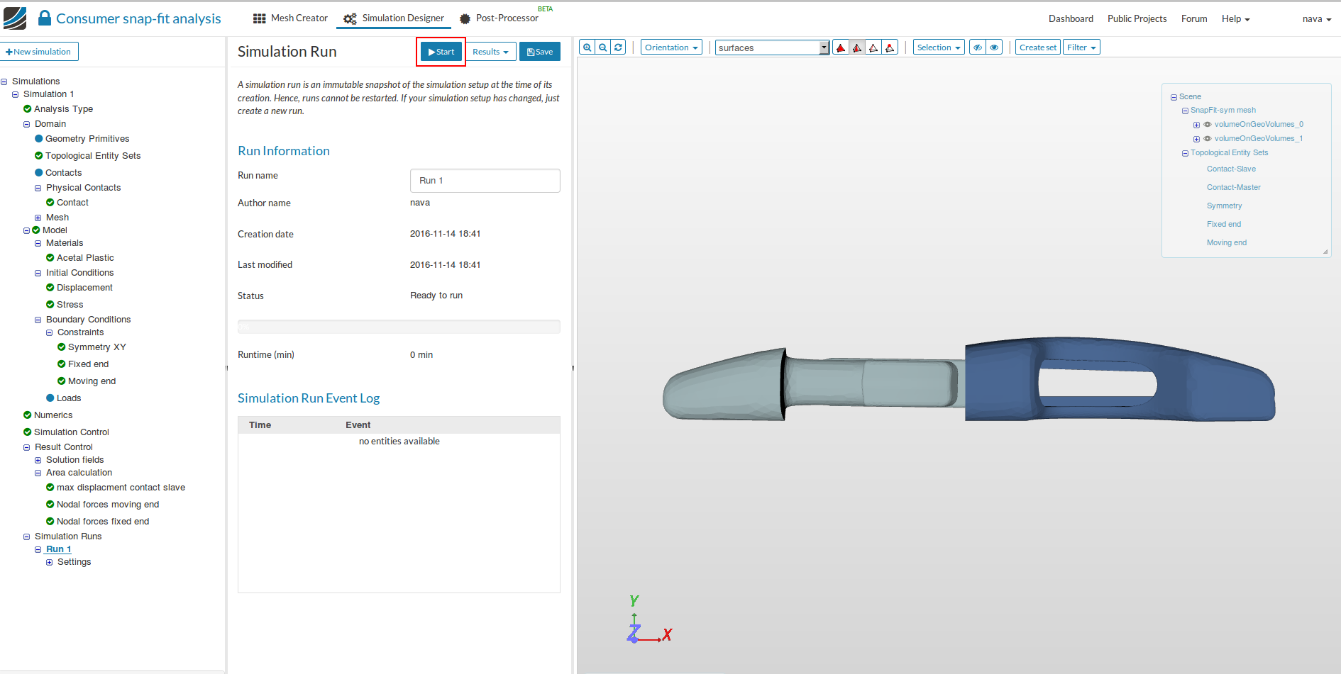
- The new run will be created under Simulation Runs. Click Start to run the simulation.
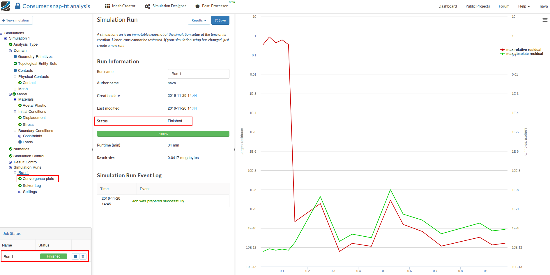
- The run takes approximately 34min to complete . After the run is finished you can see the Status as Finished and the convergence plot can be seen by selecting Convergence plots.
Post-processing
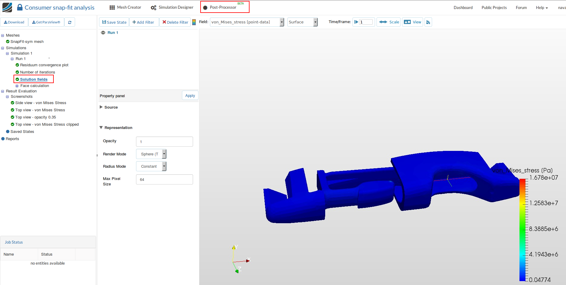
- Once the simulation is over, click on Post-processor tab to view the results and select Solution fields.
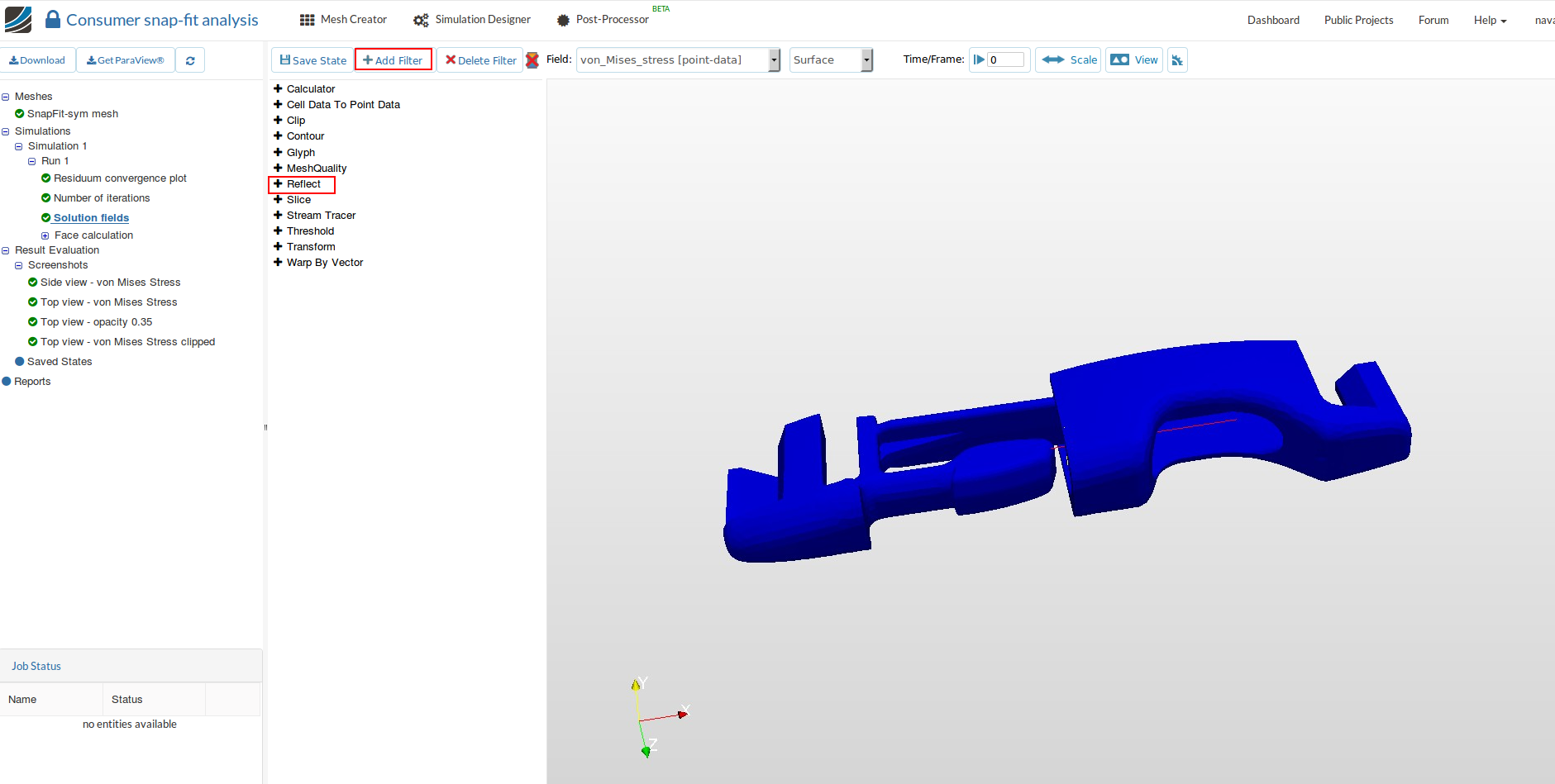
- In order to see the complete snap-fit buckle, click on Add filter and then choose Reflect filter.
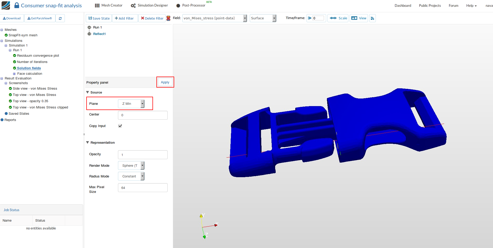
- Now we have to specify about which plane we have to reflect this result. Select Z Min for Plane and then click on Apply. The result will be now reflected about the XY plane along negative Z direction.
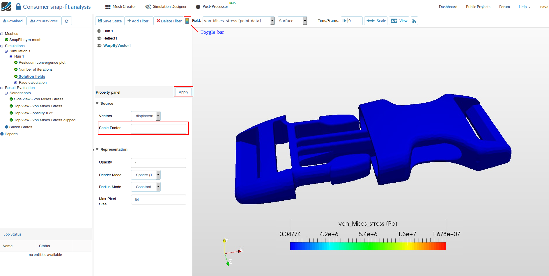
- Now we will see the deformation of the buckle with time. To do that, select Warp by Vector and specify the Scale Factor to be 1 and then click on Apply. You can view the scale by enabling the Toggle bar.
- In order to see the movement of the buckle, first hide the Run1 and Reflect1 results by disabling the Eye button. And click on Play button located at the top middle of menu bar as shown in the figure.

- The result should look like this
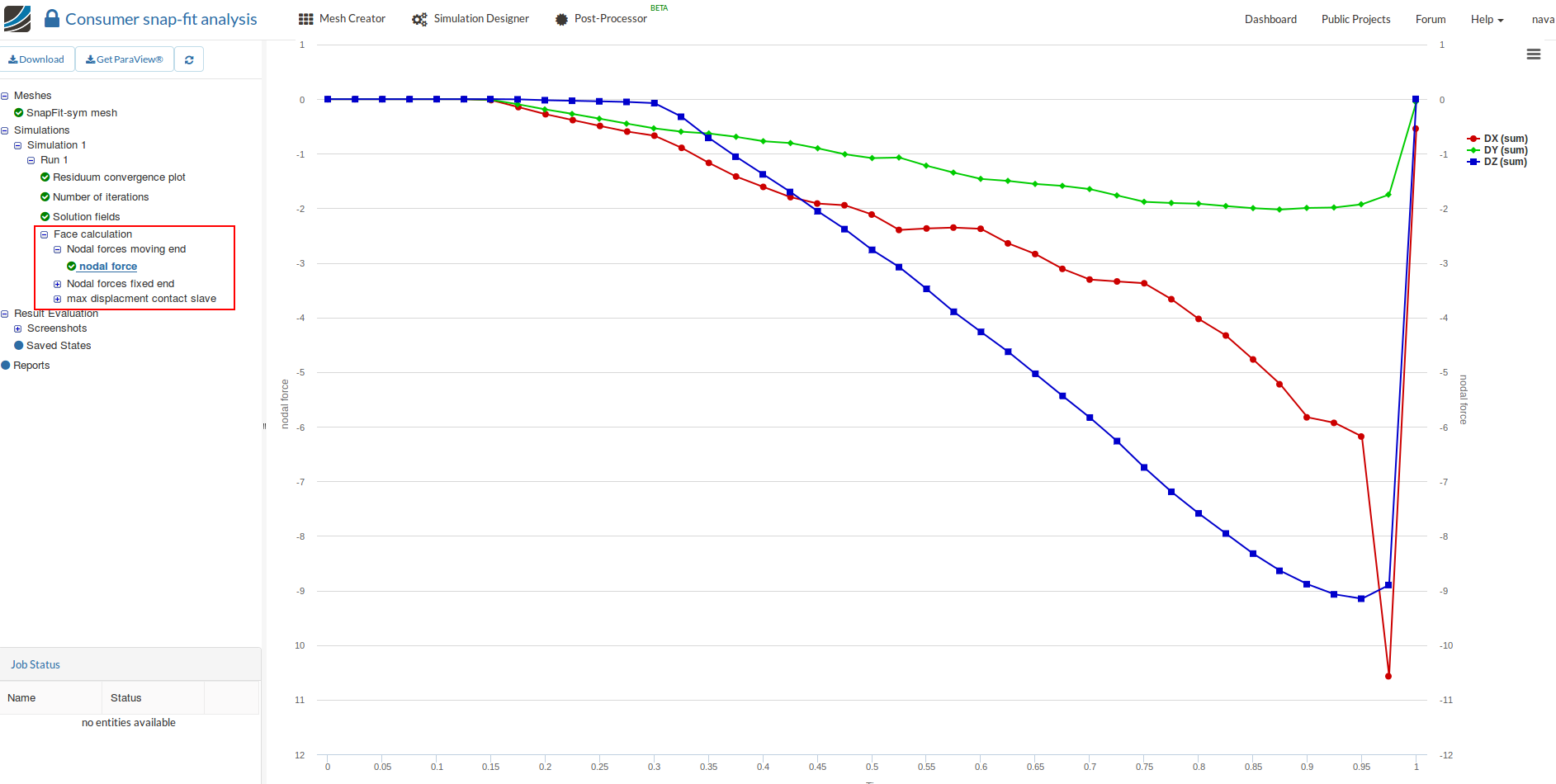
You can also see the displacement and force plots which we added as a result control items by clicking on the corresponding options available in the project tree.
Congratulations! You have successfully completed the snap fit buckle tutorial!