Simulation of unbalanced motors

Dear SimScale community,

I’m reaching out to you again.

Below you can find the project:

I’m to simulate a frame which is mounted on rubber elements and is excited by two unbalanced motors. The two motors are fixed to the frame in such manner that one rotates in clockwise the other in counter-clockwise direction giving only vertical movement to the system.

I’m curious about the magnitude of vibrations and the stresses in the structure.

So I guess Harmonic simulation is the right choice. The question is how you define the periodic excitation at one point in a direction and at an other point opposite direction?

Thank you in advance! :slight_smile:

1 Like

Hi Janos (@jhorv_th),

The forces in the x-direction cancel each other out so you only need to apply a load in the y-direction. You only need to specify the magnitude of the oscillating load. There is no need to include the sin function because the oscillation is assumed.

In your application the load generated by the eccentric mass is related to the rotational frequency. The relationship is:

The constant 0.3242 was chosen because it results in a load of 4000 N at 25 Hz (taken from your original simulation). This number is the product of the size of the eccentric mass and the eccentric offset distance (units are kg-m). For example, this could be achieved with two eccentric masses (one per motor) of 1.62 kg at an offset of 0.1 m.

You can see my copy of your project here. For the sake of simplicity I combined the two motor loads into one. Alternatively, you could split the face on which the motors are mounted and apply the two loads separately.

Here are the first six modes of vibration. These were found with a frequency analysis (and second order mesh).

Here is a frequency response plot for frequencies between 1 and 25 Hz. The multifront solver was required for frequencies below 7 Hz. I’m not sure why this is. Richard (@rszoeke) might be able help out here.

From the result control items in your project it appears that you are interested in mode 6 (oscillations in the z-direction). Is the structure constrained sufficiently in the X and Y directions such that none of the other modes are present?

On face value there seems there is a problem with your material properties. Your elastic modulus for rubber (77390 Pa) seems very low. Your frame material has an elastic modulus of steel but a very low density (560 kg/m3). I have used you material properties but you should check that these make sense for your application.

Hand calculations for the first and sixth modes can be found here.

Does this answer your question? Please let me know if you need further help.

Regards, Ben

6 Likes

Hi @jhorv_th @BenLewis!
First, thanks Ben for the great help and explanation!

Regarding the problem with the MUMPS solver, I guess a quick excursus would be helpful:

The MUMPS solver provides methods to estimate the quality of the solution of the linear system. On SimScale it can be controlled with the parameter Linear system relative residual of the MUMPs solver.

When doing error analysis for the solution of a linear system
$$ Ku = f $$

the main interest is the relative forward error {||\delta{u}||} \over {||u||}. It is the relative difference of the computed solution u^* from the actual (unknown) solution u. In most cases this error is unknown, but it can be estimated with an inverse approach using the backward error and the condition number of the solution matrix.

The backward error \eta(K,f) measures which modification \delta{f} to the RHS f would be needed to actually have u^* as the exact solution:
$$Ku^* = f + \delta{f}$$
The backward error is mainly introduced by rounding errors and should ideally be in the order of the machine precision (1e^{-15}).

The condition number indicates how sensitive the solution is to changes in the input variables, e.g. how much input errors influence output errors. For high condition numbers (\kappa(K)>1e^{10}), even small variations in the input can lead to drastic changes in the solution.

Putting both together we can state:
$$ {{||\delta{u}||} \over {||u||}} < C* \eta(K,f)* \kappa(K) $$
with C being some constant, thus the right hand side being an upper bound for the forward error.

Now if the product \eta(K,f)* \kappa(K) becomes larger than the user defined Linear system relative residual, the solver stops and ends with a message that the desired residual of the MUMPS solver could not be reached.

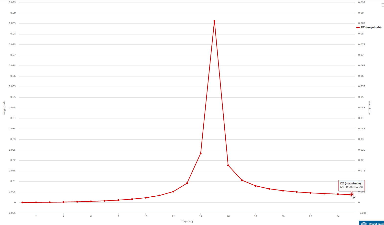
In this case here, we know that the error appears only below a certain frequency. As the matrix stays the same, we know that the reason must be an increasing backwards error for smaller frequencies, which is a common phenomena as the overall forces get lower, rounding errors get more important.

Now regarding the solution of this problem, there are several possibilities:

  • increase the residual. A value of 1e-3 is not very uncommon and sometimes needed to be able to successfully run the analysis.
  • turn off the relative residual check: using a negative value will deactivate the check. Since in this special case we already have a reference solution using MultFront we can be pretty confident to remove the test. (after I did it the solution time dropped from 100min with MultFront to 30min with MUMPS, giving the exact same results for the first 5 significant digits).
  • change the settings of the MUMPS solver. Generally one could play with the selection of the renumbering tool, matrix type, in case of an Harmonic Analysis the possible choices are limited however
  • improve the mesh quality. In this particular case I guess a big part of the problem is related to the bonded contact between the rubber and the frame where we have very high differences in mesh density on the master and slave side.
  • check the coherence of your input data. Here, as already pointed out by @BenLewis, the stiffness of the rubber seems very low. In combination with the high Poissons ratio (0.499) and the very high stiffness of the other contact partner, steel, this will lead to a bad conditioning of the system matrix.

I hope this helps to understand the error reason and points to possible solutions.
Best,
Richard

4 Likes

Hi @BenLewis @rszoeke,

thanks guys, your helpfullness is awesome!

I need some more time to digest what @rszoeke said. :smiley:

@BenLewis:

We have 2 times 80 kg*mm unbalanced motors @25Hz. So in fact they provide together approx. 4000N excitation.

Yes, the structure is constrained by elastic mounts which prevent X, Y motion.

The density of steel is modified because the mass is indeed 60kg (as you also calculated). Actually it is not a block of metal rather some sheet metal construction. The elastic modulus of rubber springs was modified to meet our spring constant.

For the relation of spring constant and elastic modulus I found the following formula:
k = Y*A/L

Reference Is There A Relationship Between Young's Modulus And Spring Constant? | Physics Forums

But I must have miscalculated because I wanted to set 410 N/mm. Oups. :smiley:
Is there any direct way in SimScale to define the spring constant for a material? That would ease things.

Below I’ll provide my hand calculations. The expected stroke should be around 7mm.


P.s.: what software did you use for the frequency plot?

Thank you guys again! :slight_smile:

1 Like

Hello @jhorv_th,
you can actually use an elastic support constraint which provides directly the possibility of defining the spring constant
(even different stiffness for x-, y- and z-direction.
For an example you can have a look at this two projects:

Best,
Richard

Hi @rszoeke,

I don’t think the elastic support constraint is available in the frequency and harmonic analysis types.

Regards, Ben

Sorry @jhorv_th,
@BenLewis is absolutely right, this feature is currently not available for harmonic or frequency analysis.
Maybe it’s worth a feature request? At least for the harmonic analysis it would not be too difficult to add.
Best,
Richard

Hi @jhorv_th,

As the structure is constrained from motion in the X and Y directions we can use symmetry about these two planes (quarter model).

I have shelled the model so that the resultant weight is approximately 60 kg for standard steel density.

The formula for the total excitation load is:

0.082(2pif)^2

For a quarter model this becomes:

0.08/2*(2pif)^2

The formula I used to calculate the elastic modulus is:

E = k*h/n/l/w

where:
k = desired spring constant (410e3 N/m)
h = height of elastic element (0.05 m)
l = length of elastic element (0.091 m)
w = width of elastic element (0.049 m)
n = number of elastic elements (8)

therefore:
E = 410e3*0.05/8/0.091/0.049 = 754,680 Pa

The first mode of vibration is now in the expected Z-direction and occurs at 14.8 Hz. From hand calculations I get 13.0 Hz. I’m not sure why there is a discrepancy.

Your hand calculations show you are expecting a stroke is 7.4 mm. The results from the harmonic analysis show a displacement of 3.8 mm. The total stroke is twice this value because the displacement occurs in both directions. Therefore the total stroke is 2 x 3.8 = 7.6 mm (pretty close to hand calculations).

In the previous example I used Excel to plot the frequency response data (downloaded from the SimScale post processor). By setting the relative residual to -1 (thanks @rszoeke for the tip) I can now solve the entire spectrum from 1 Hz to 25 Hz in one simulation. So the results can now be viewed directly in the SimScale post processor. The frequency response plot now looks like this.

I’ve updated my project here.

Regards, Ben

4 Likes

Hi @BenLewis,

awesome! I’m absolutely happy that the calculated and simulated values for stroke are so close!

In the mean time some parameters have changed so I’ll need to re-evaluate here and there but I’m quite confident that I can solve it based on your project!

Thank you guys again! :slight_smile:

Cheers!

5 Likes