Air Conditioning and Ventilation Webinar
Contamination control design of a Clean room
Air Conditioning and Ventilation Workshop (Session 4 ) ― Contamination Control of a Cleanroom
Session - 4 Learning Assignment: Ventilation Exhaust Analysis
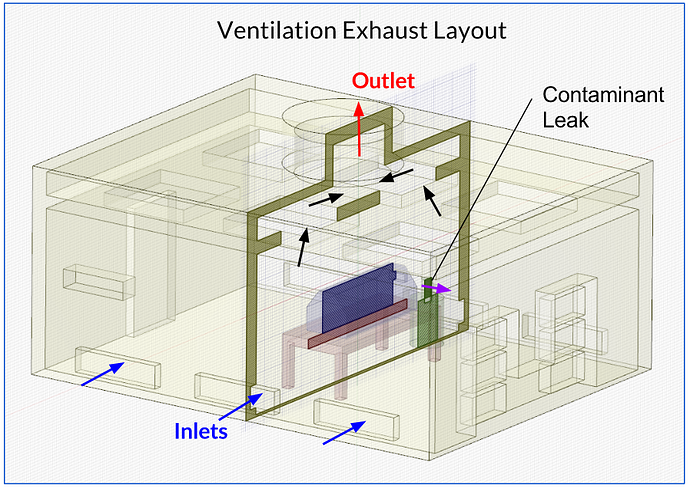
Description: The assignment will be to simulate a Ventilation Exhaust setup for a Clean Room with a gas leak from a container. The sketch below shows the setup with ‘Flow Inlets’ along the floor and central circular ‘Outlet’ on the ceiling. The ceiling has 6 open rectangular sections from which the flow exits the room and is exhausted out through the central outlet.
Import the project by clicking the link below (Ctrl+click to open in new tab).
Project Link: SimScale Login
Once the project is imported, the workbench is automatically opened. Then follow the steps below for setting up an incompressible simulation.
Step-by-step
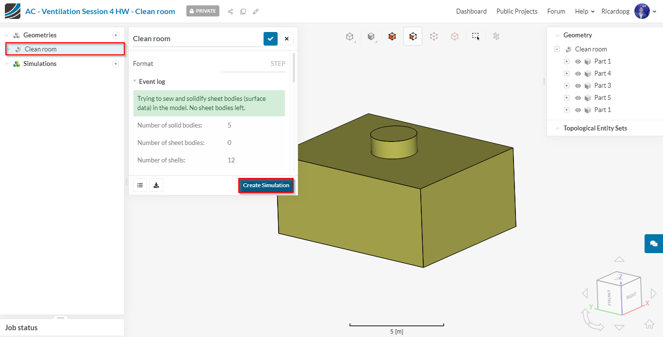
Please select the Clean room geometry and click on Create Simulation.
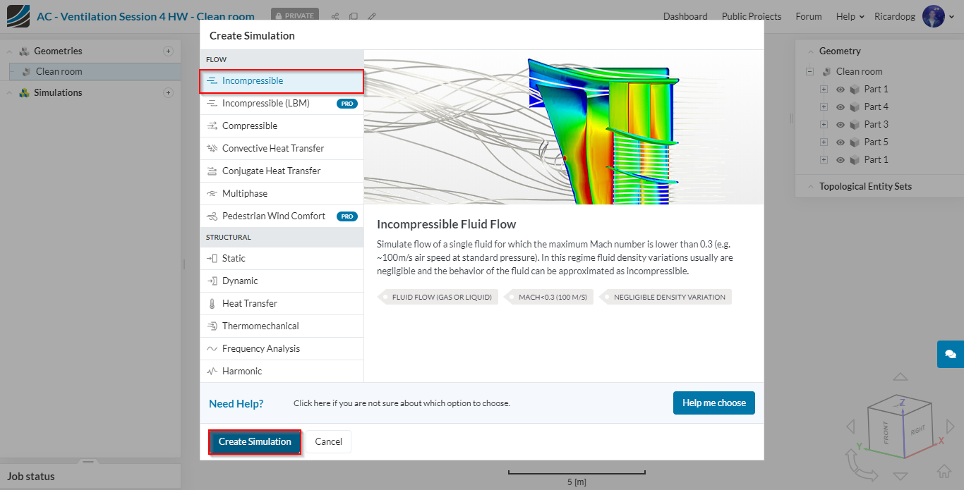
A window with different analysis types will appear. Choose Incompressible and proceed by clicking Create Simulation.
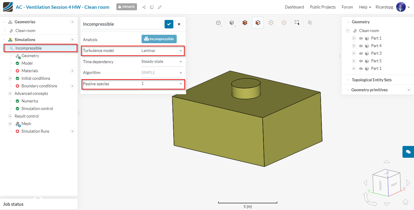
On the left-hand side of your screen, the simulation tree will appear. Each one of the tabs marked in red needs to be filled in order to run the simulation.
First, let’s start by changing the settings of our Incompressible simulation. Please change Turbulence model to Laminar. Also change Passive species to 1. This passive species will be the contaminant.
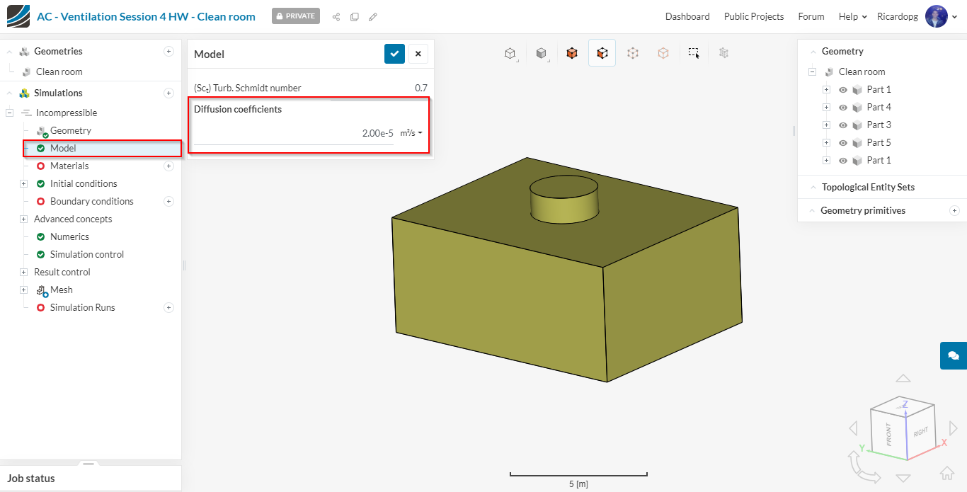
The passive scalar will spread through the flow region by means of convection and diffusion. In Model, we can assign a Diffusion coefficient. This coefficient is usually given for a binary of materials (e.g. air and CO). The coefficient for some binary gas mixtures can be found here.
In our case, we will assign it a value of 0.00002 {m² \over s}:
Meshing
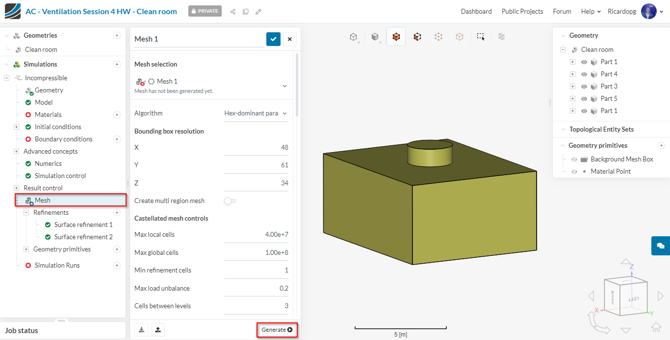
In the simulation tree, click on Mesh. Change the mesh Algorithm to Hex-dominant parametric (Only CFD):
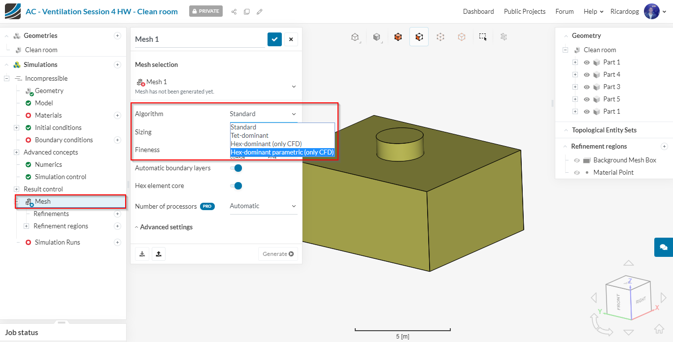
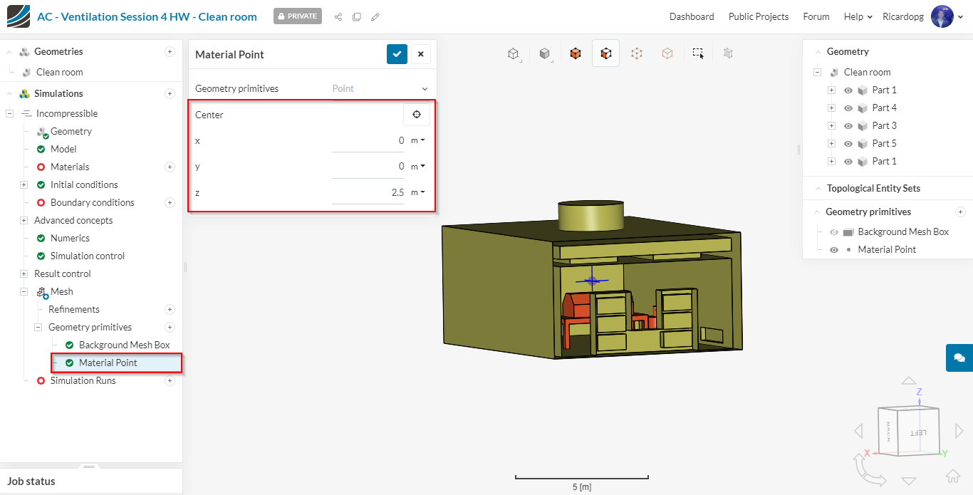
Now in the simulation tree, just under Mesh, there’s an entry for Geometry primitives. Please expand it by clicking in the + sign next to it. There will be 2 automatically created primitives: Background Mesh Box and Material Point.
Material Point lets the meshing algorithm know what region you want to be meshed. Give a click on it and adjust the coordinates as shown below:
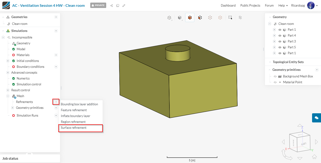
Surface refinements are up next. To add a refinement, click on the + icon next Refinements and select the desired type of refinement.
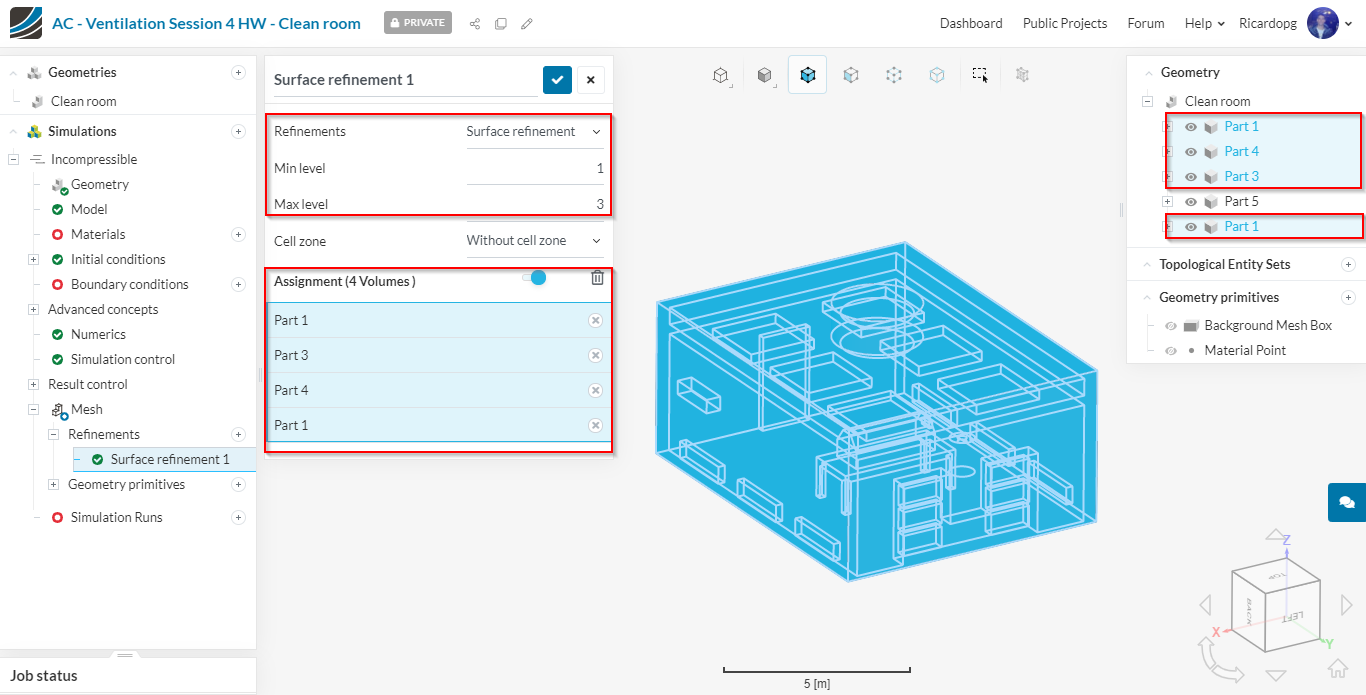
For the first Surface refinement, we will assign 4 volumes (just click on the volumes in the right-hand side panel in your screen to select the volumes). By assigning a volume to a surface refinement, all faces within that volume will be refined as requested.
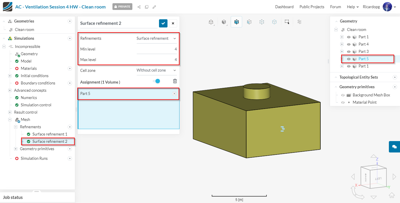
We will create another Surface refinement for Part 5 now:
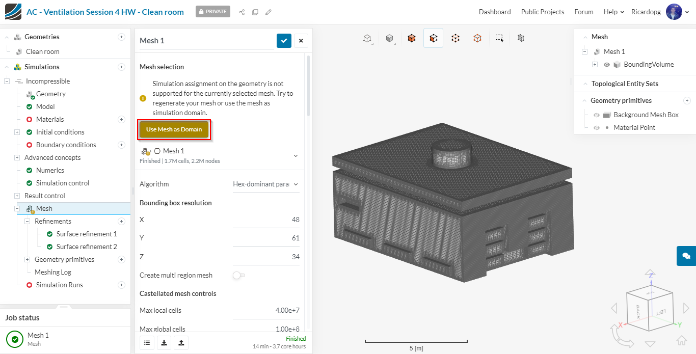
The mesh is now ready to be generated. In the simulation tree, click on Mesh and then on Generate (towards the bottom of the screen). The number of processors that will be used is automatically optimized by the algorithm.
It takes about 14 minutes for the mesh to be generated. When it’s ready, make sure to click on Use Mesh as Domain.
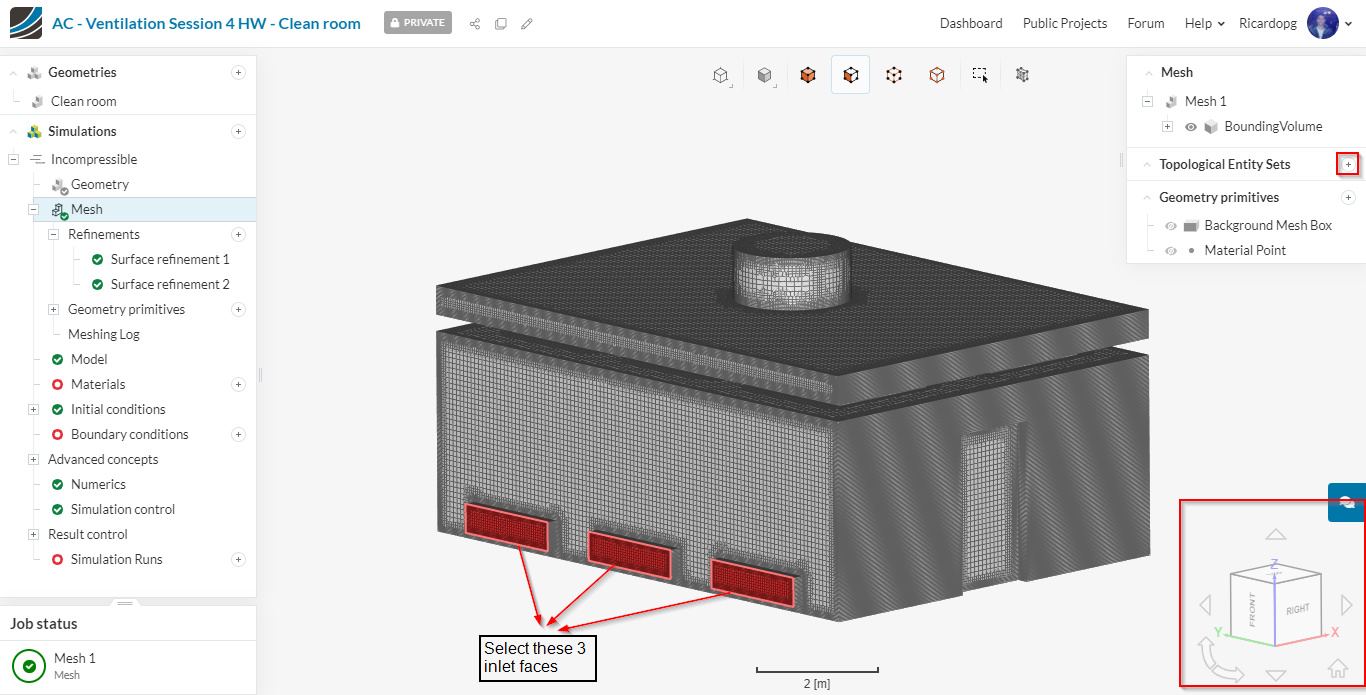
Topological Entity Sets
Topological entity sets are used to make groups of faces. They’re useful to, later on, set up boundary conditions and result controls. A new Topological Entity Set is assigned as follows:
- Left click on the face or faces that will constitute a topological entity set;
- On the right-hand side panel, next to Topological entity set, click on the + button;
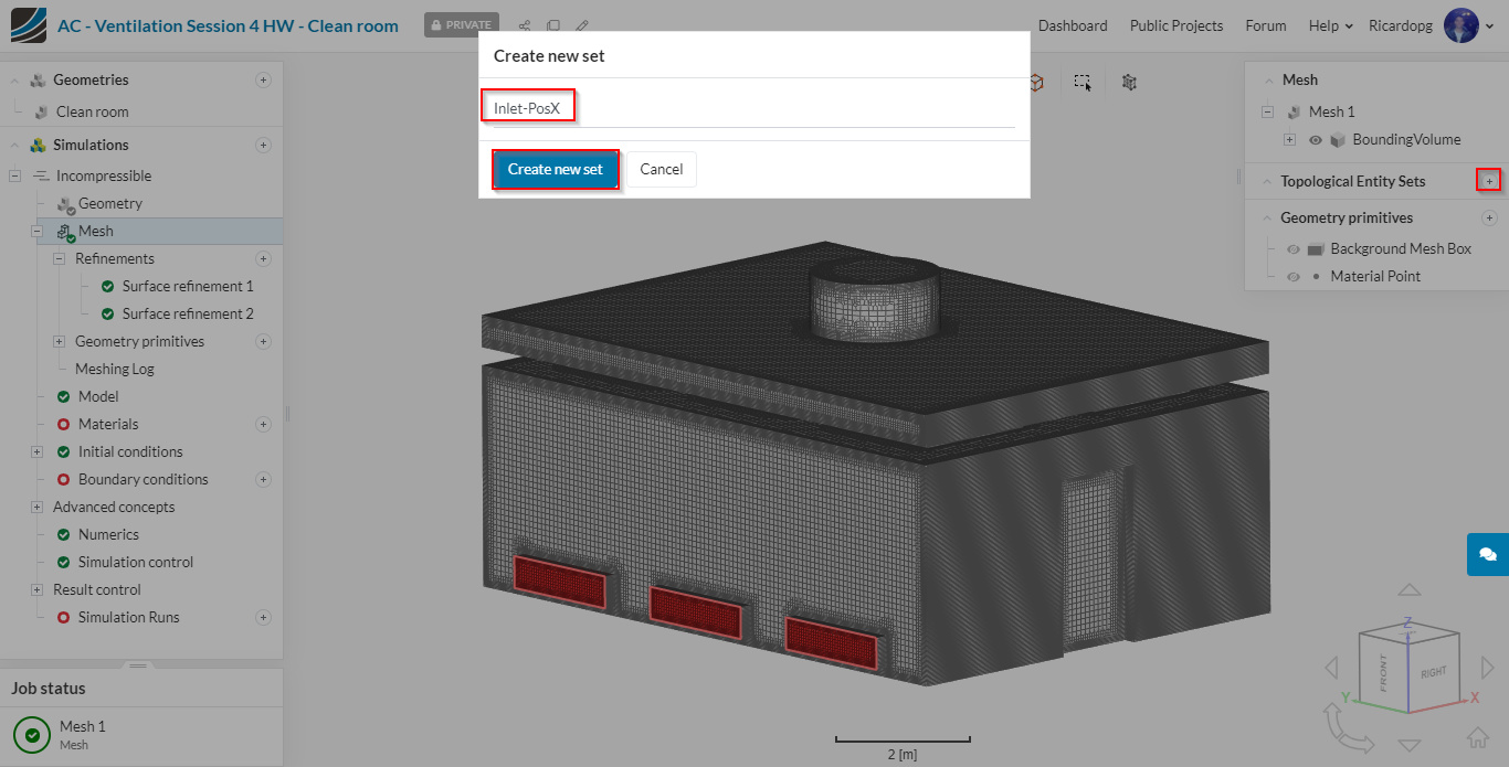
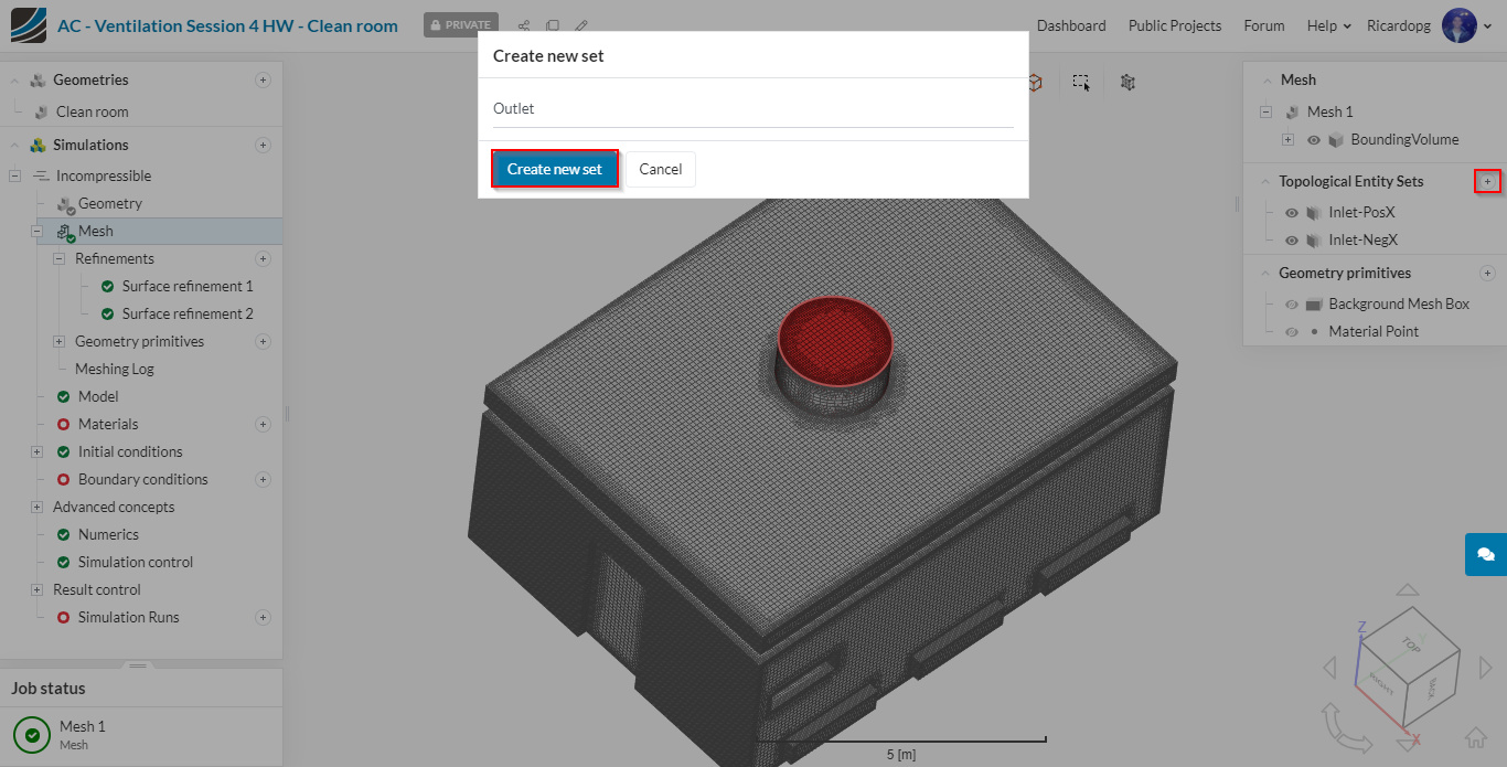
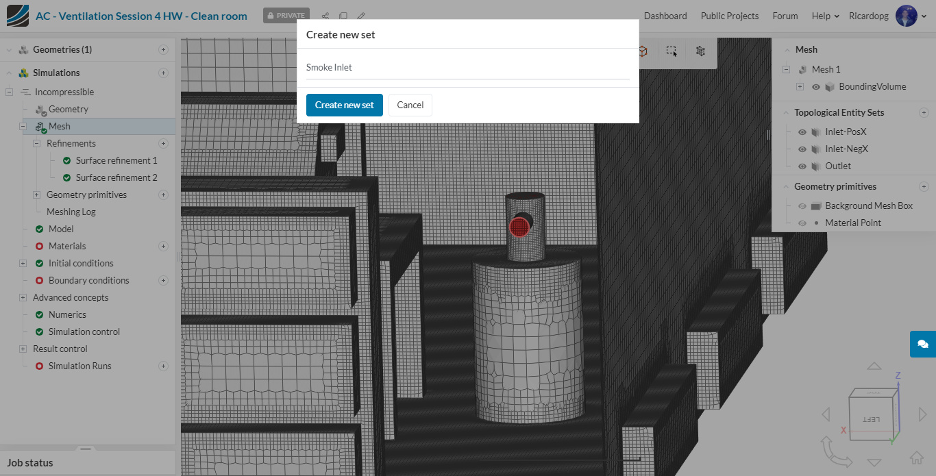
- Name your entity set as you deem suitable and click on Create new set.
Please create a topological entity set named Inlet-PosX as shown below:
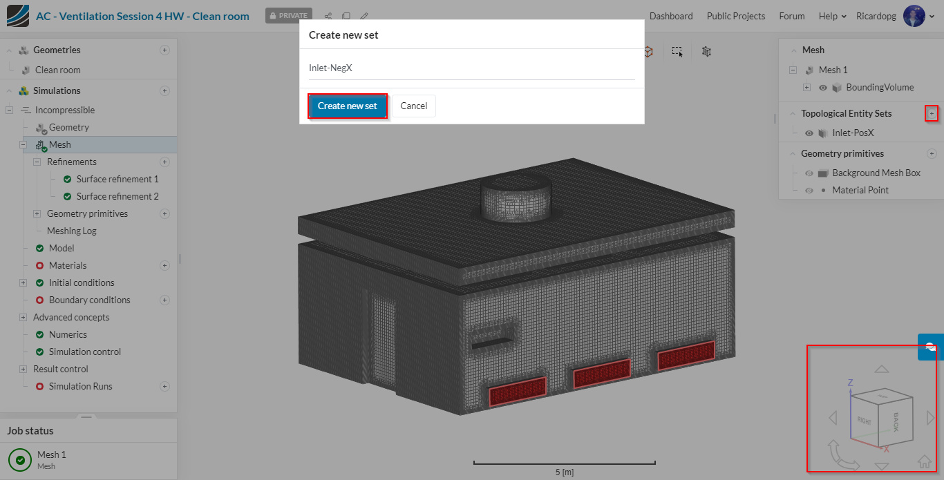
Please create a topological entity set named Inlet-NegX as shown below:
Select the top circular face and create the Outlet topological entity set:
Now we are going to select one of the internal faces to create the Smoke Inlet topological entity set. In order to visualize this internal face, we have to hide one of the external walls:
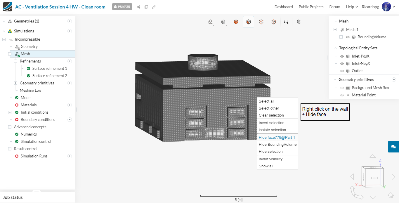
.
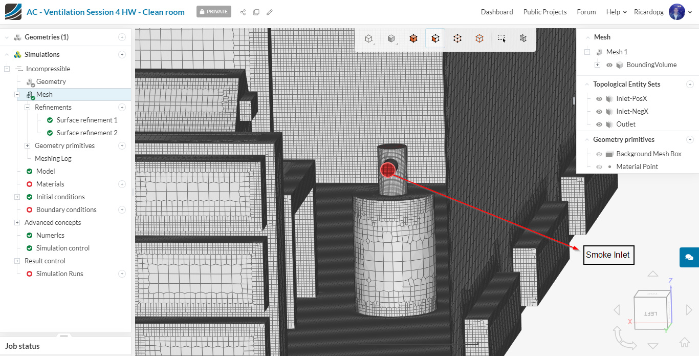
.
We will now proceed to making a Walls topological entity set. Follow the steps below:
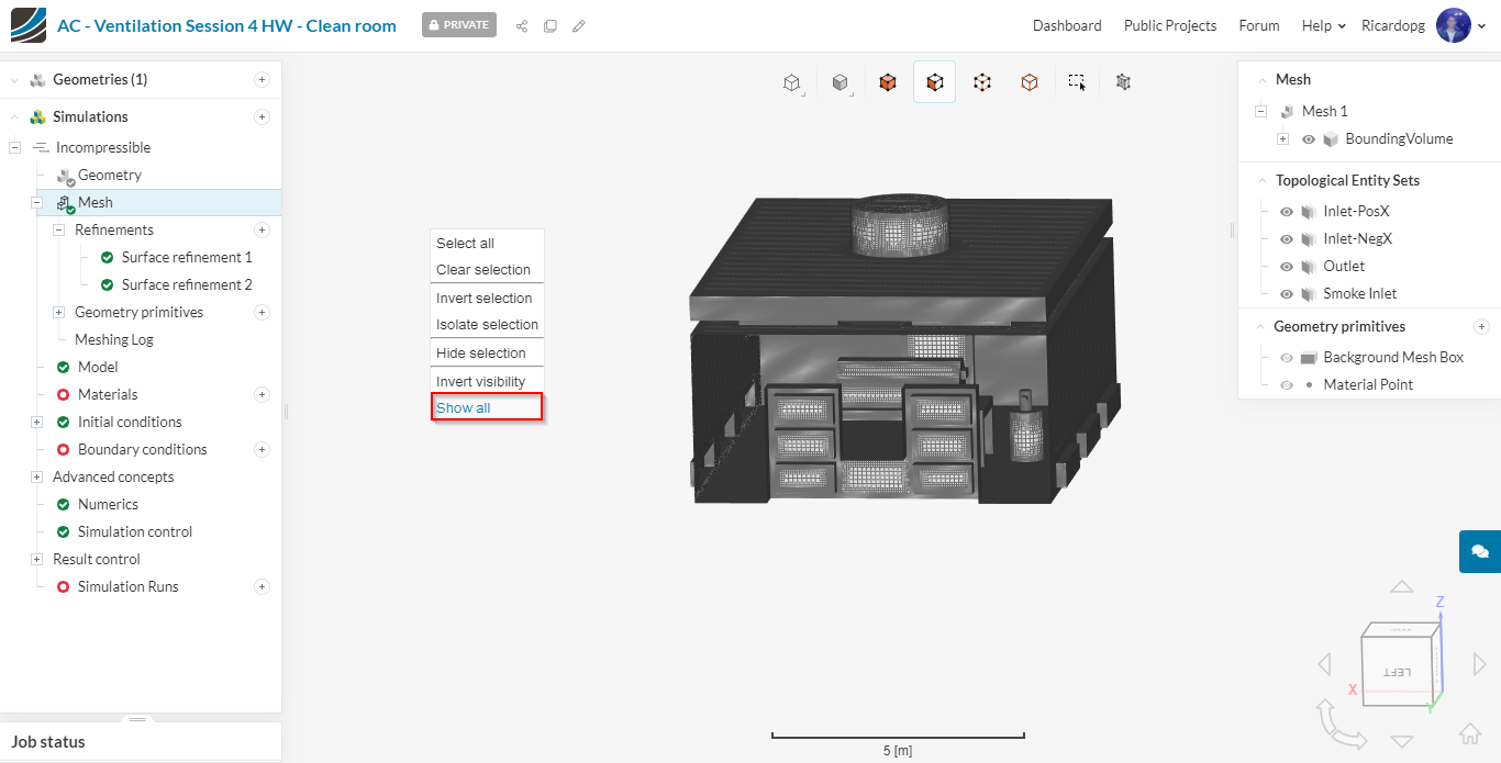
First, please right click in the viewer and select Show all to show all faces.
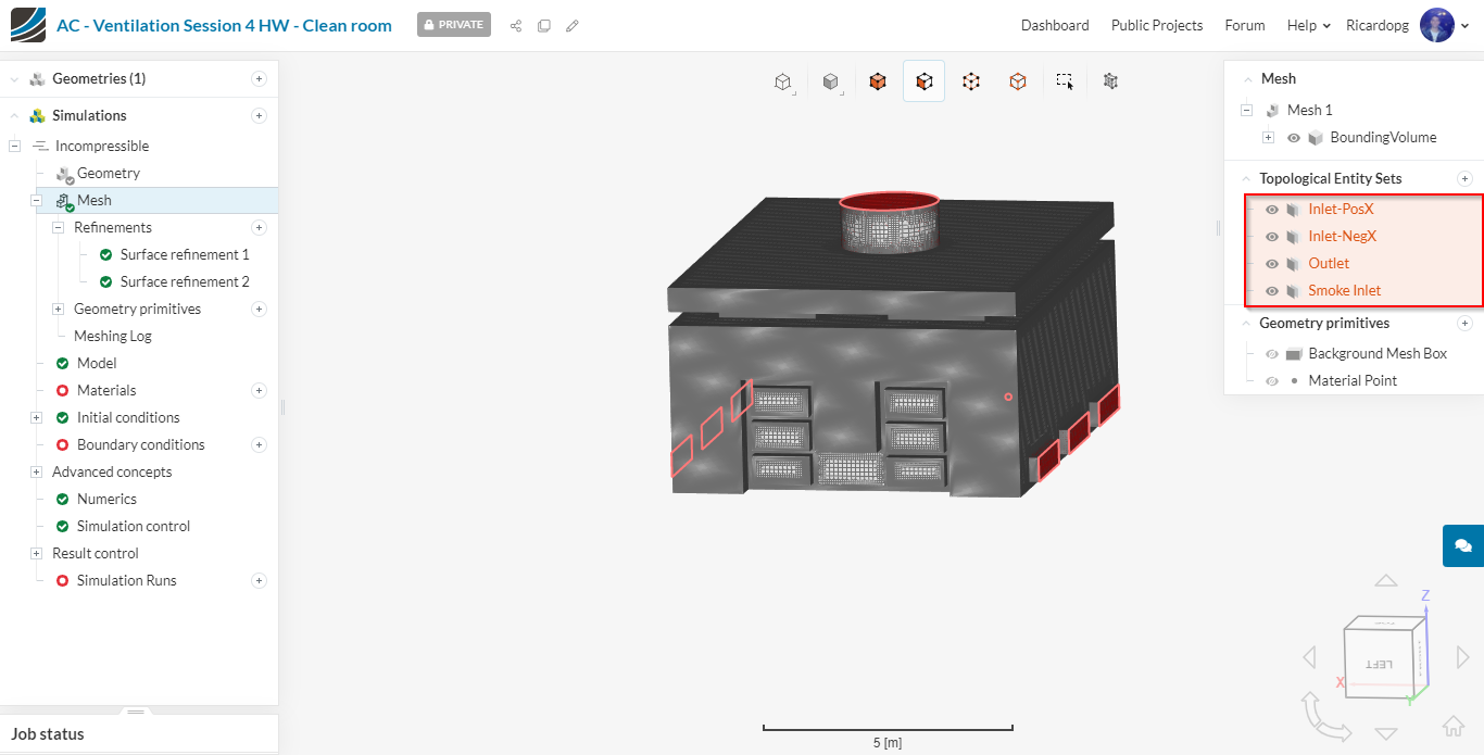
Then select all 4 topological entity sets that were created previously:
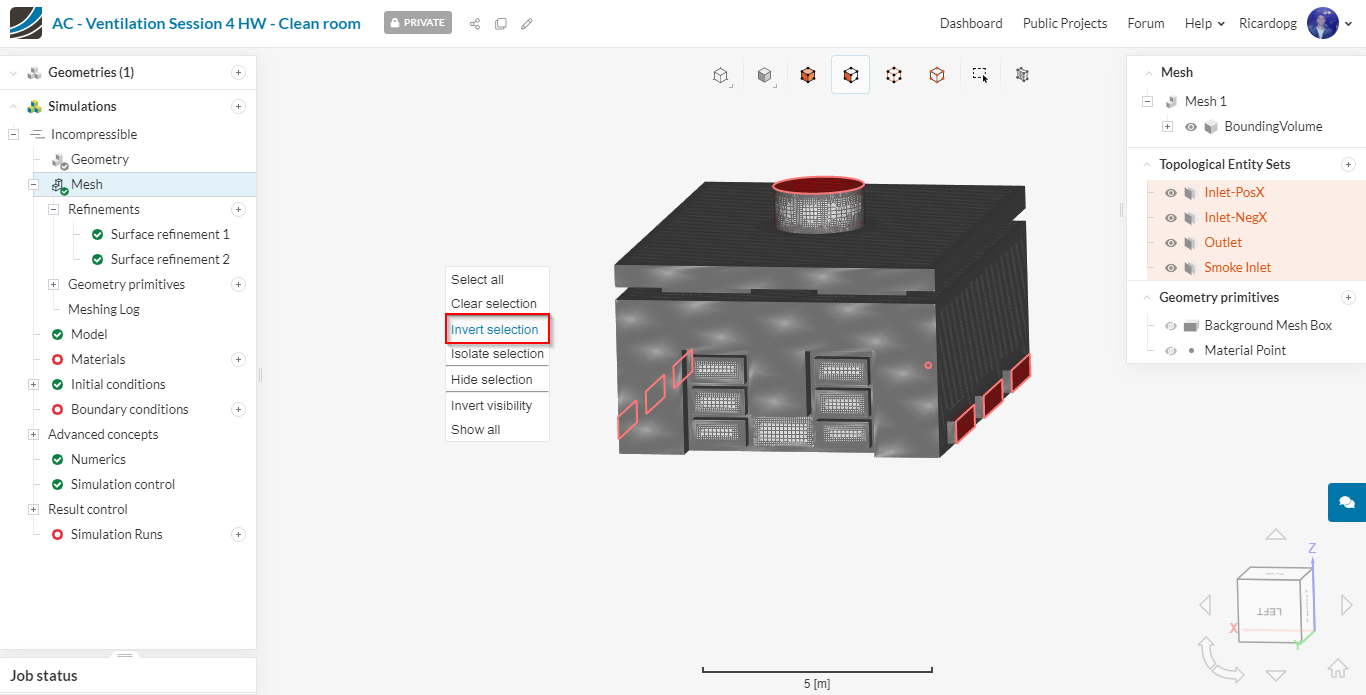
Now right click in the viewer again and select Invert selection.
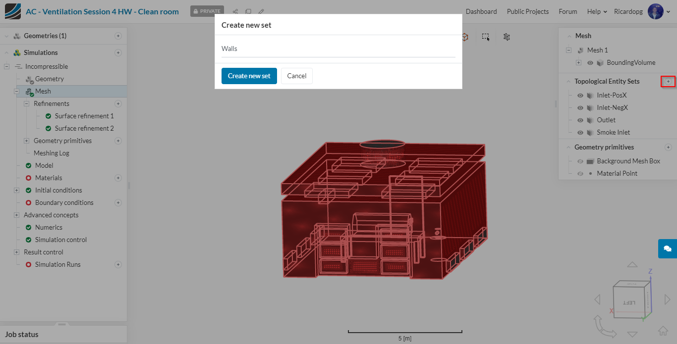
As a result, conviniently, all previously unselected faces will now be selected. You can proceed to creating the Walls topological entity set:
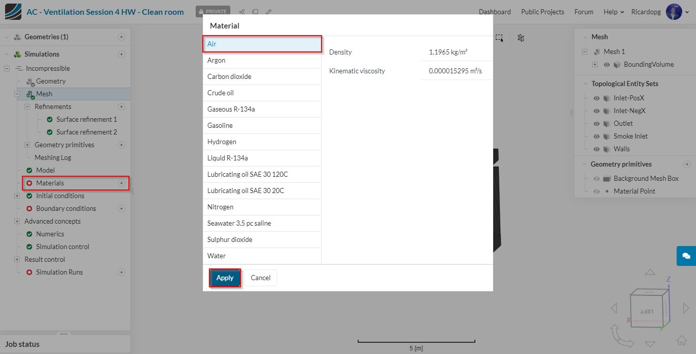
Proceeding to Materials in the simulation tree. Select Air from the materials library and hit Apply:
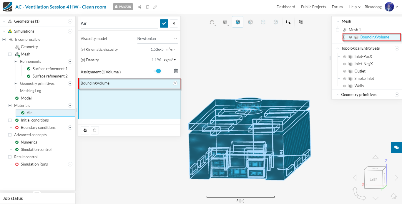
Air will then be automatically assigned to the BoundingVolume.
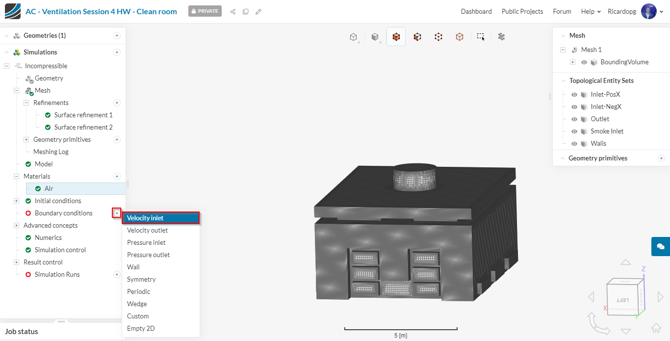
Boundary conditions
A boundary condition is created by clicking on the + icon next to Boundary conditions and selecting the appropriate type. In order to create the Inlet-PosX boundary condition, select Velocity inlet:
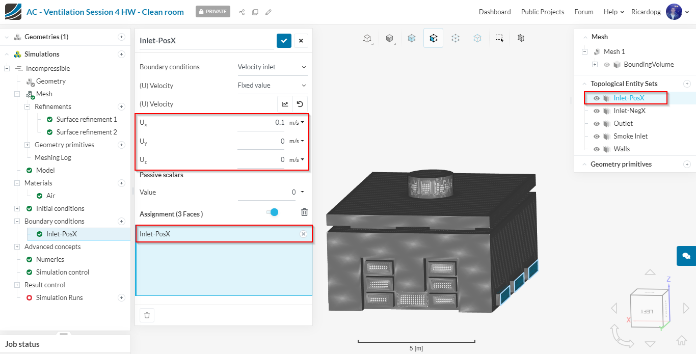
Please input a +0.1 {m \over s} velocity in the X direction and assign the Inlet-PosX topological entity set that was previously created.
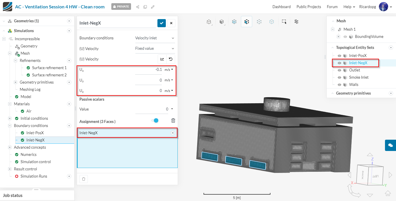
Following the same logic, now create a similar boundary condition for the Inlet-NegX, this time with a -0.1 {m \over s} velocity in the X direction:
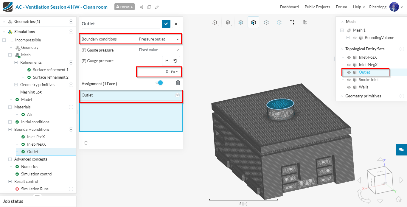
A pressure Outlet condition can be created as shown:
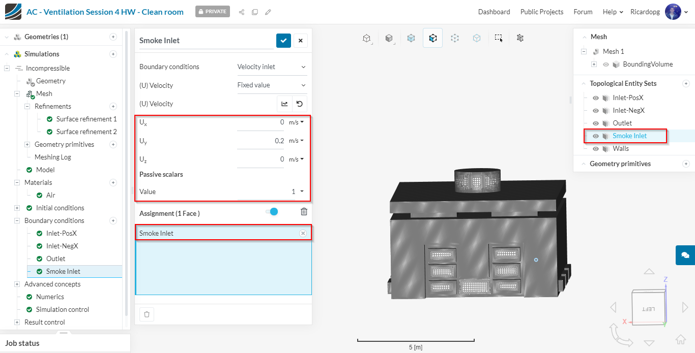
Proceeding to the Smoke Inlet, it will be a velocity inlet type with +0.2 {m \over s} in the Y direction. Passive scalars will have a value of 1 in this boundary condition:
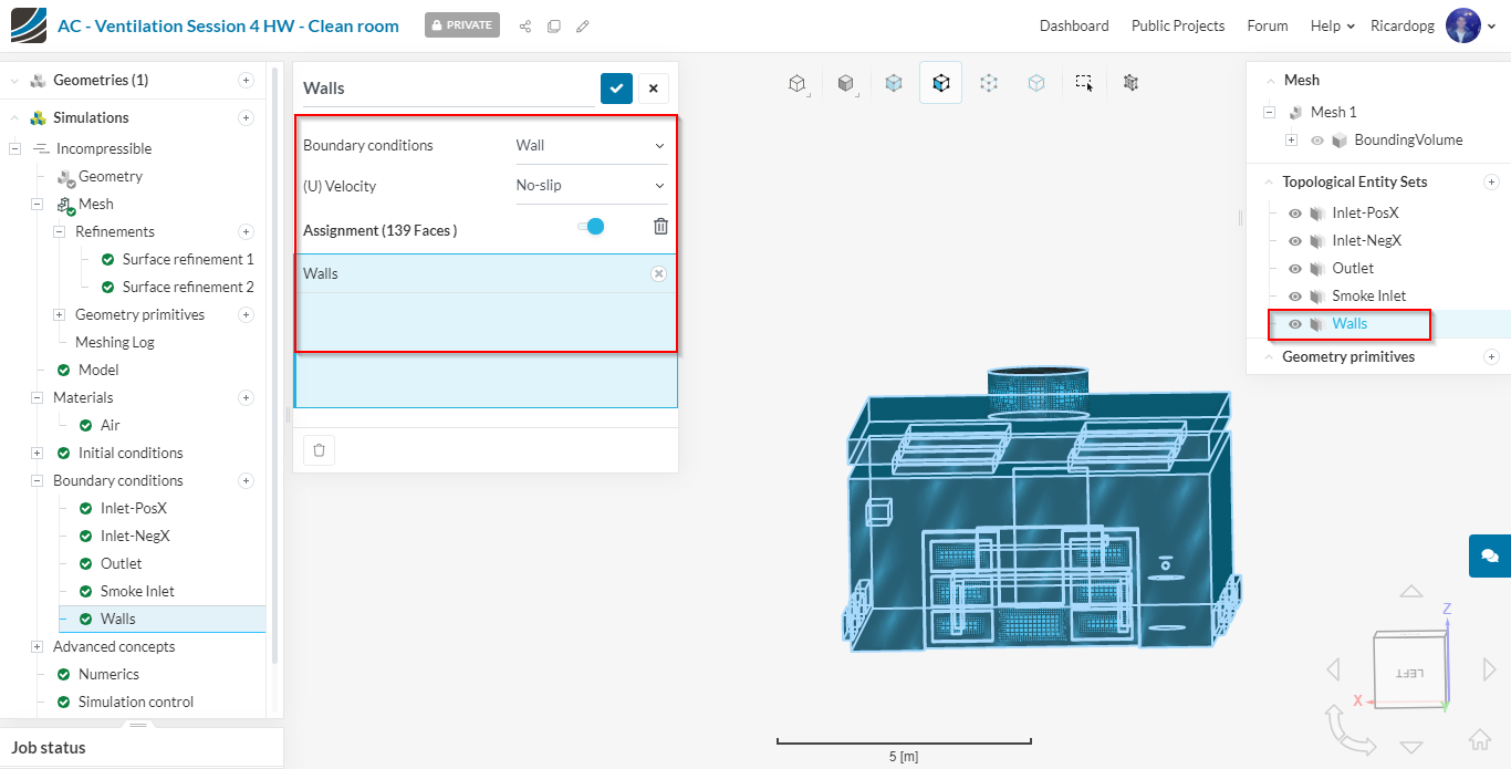
Finally, Walls is going to be a No-slip for velocity:
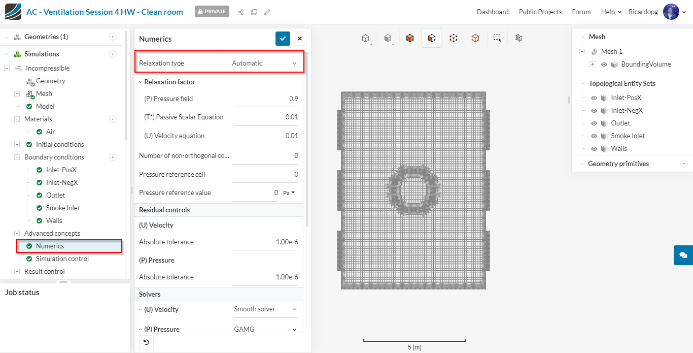
In the simulation tree, please navigate to Numerics and make sure the Relaxation type is Automatic:
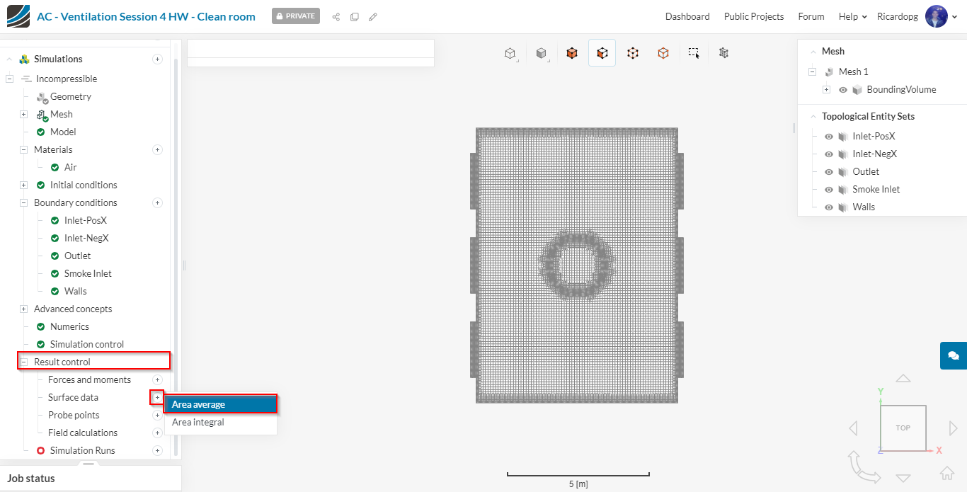
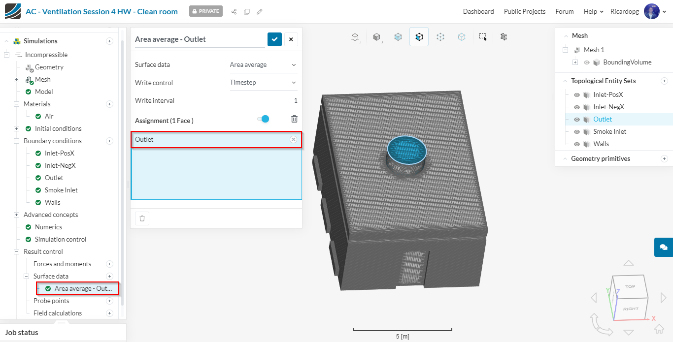
To help us assess convergence, let’s set a Result control. It will be an Area average at the Outlet:
In Simulation control, please toggle Potential foam initialization on.

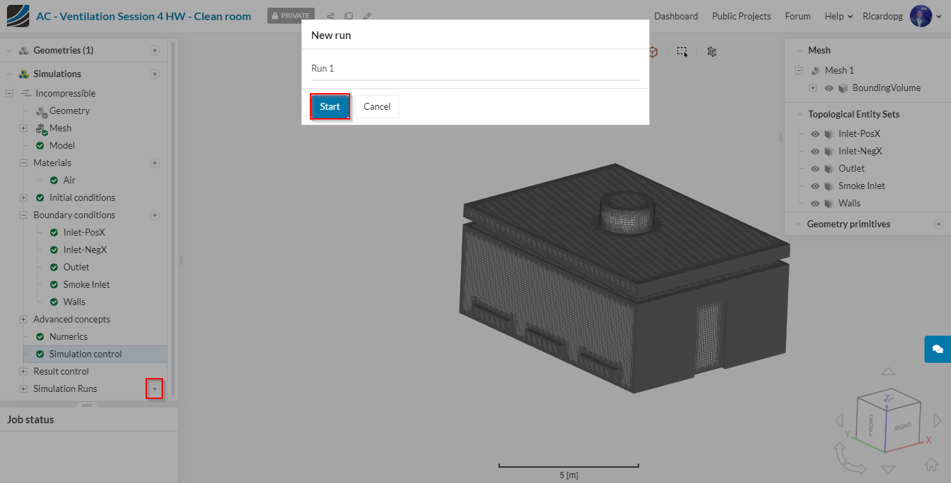
Now we’re ready to run the simulation.
Post-processing
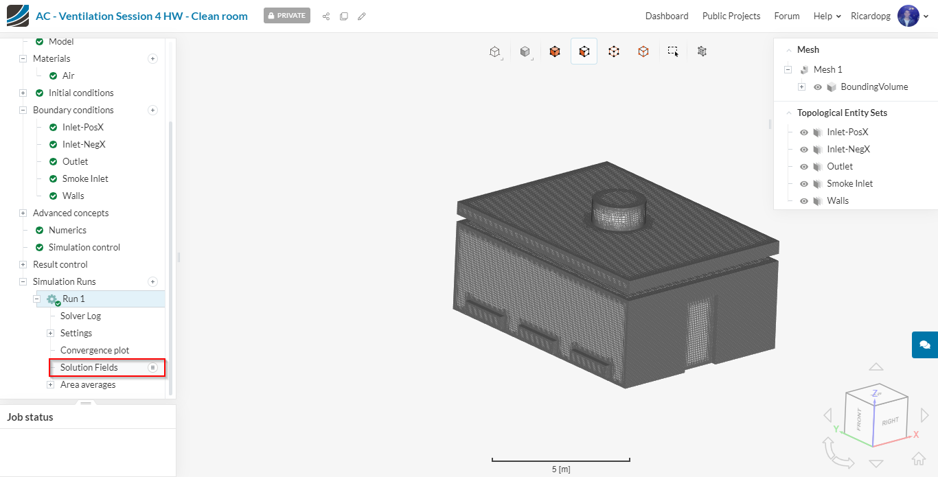
When the simulation finishes running, please head over to the post-processing environment by clicking on Solution fields.
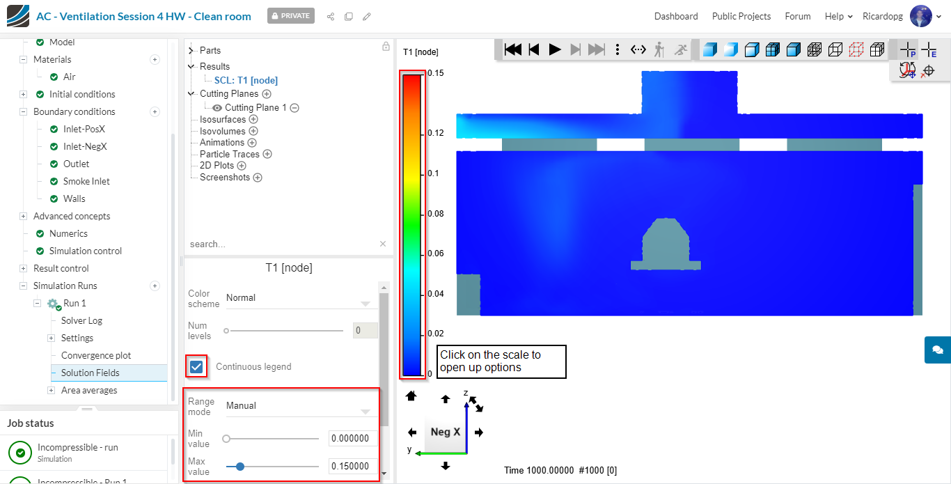
Now, in the post-processing environment, let’s slice our geometry by using a Cutting Plane. Select the X direction to make it normal to the X axis.

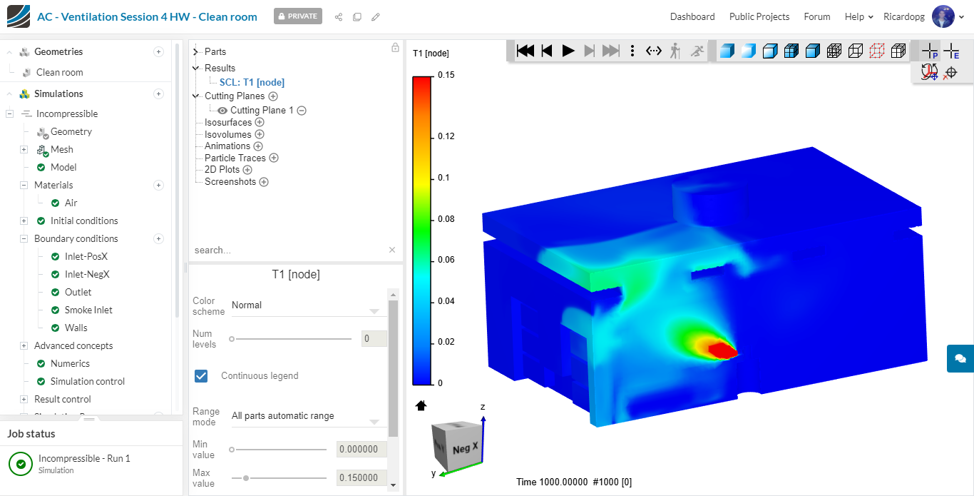
We want to analyze the passive scalar concentration T1. The 0 to 1 scale range isn’t very representative of our domain. So let’s adjust it to 0 - 0.15 by clicking on the scale and changing its configurations:
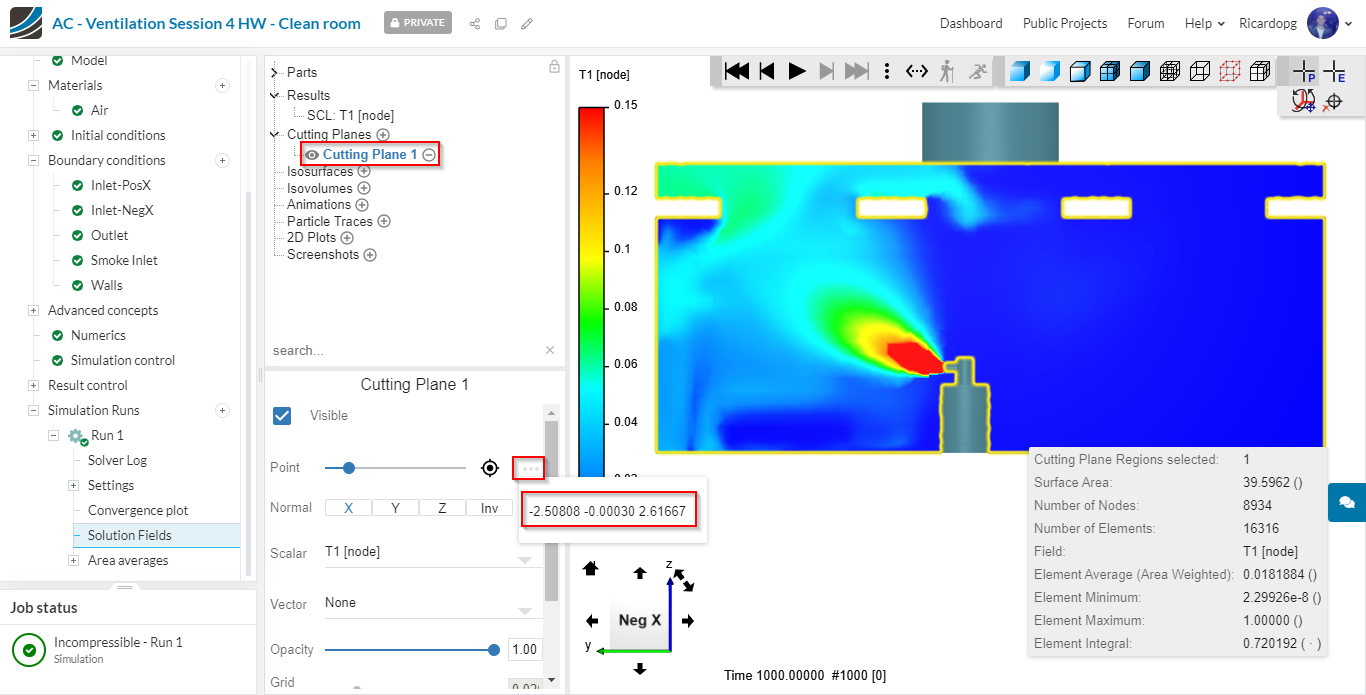
Let’s take a look at the smoke inlet. Back to Cutting Plane 1, adjust the sliding bar next to Point to show the inlet. Alternatively, you can click on the three dots and input the following coordinates:
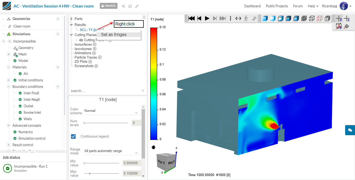
By default, only the cutting plane will be colored. We can change it by setting T1 as fringes:
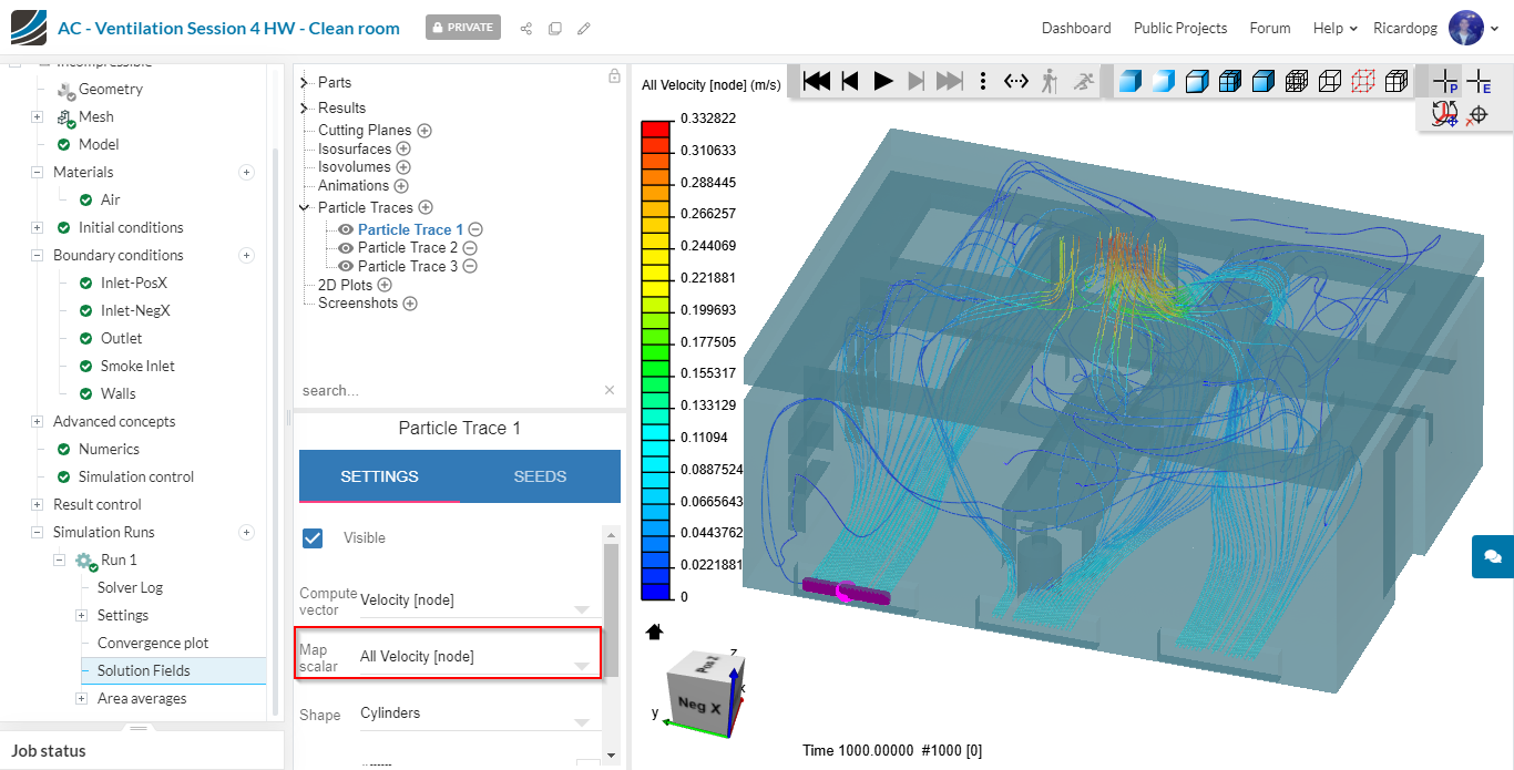
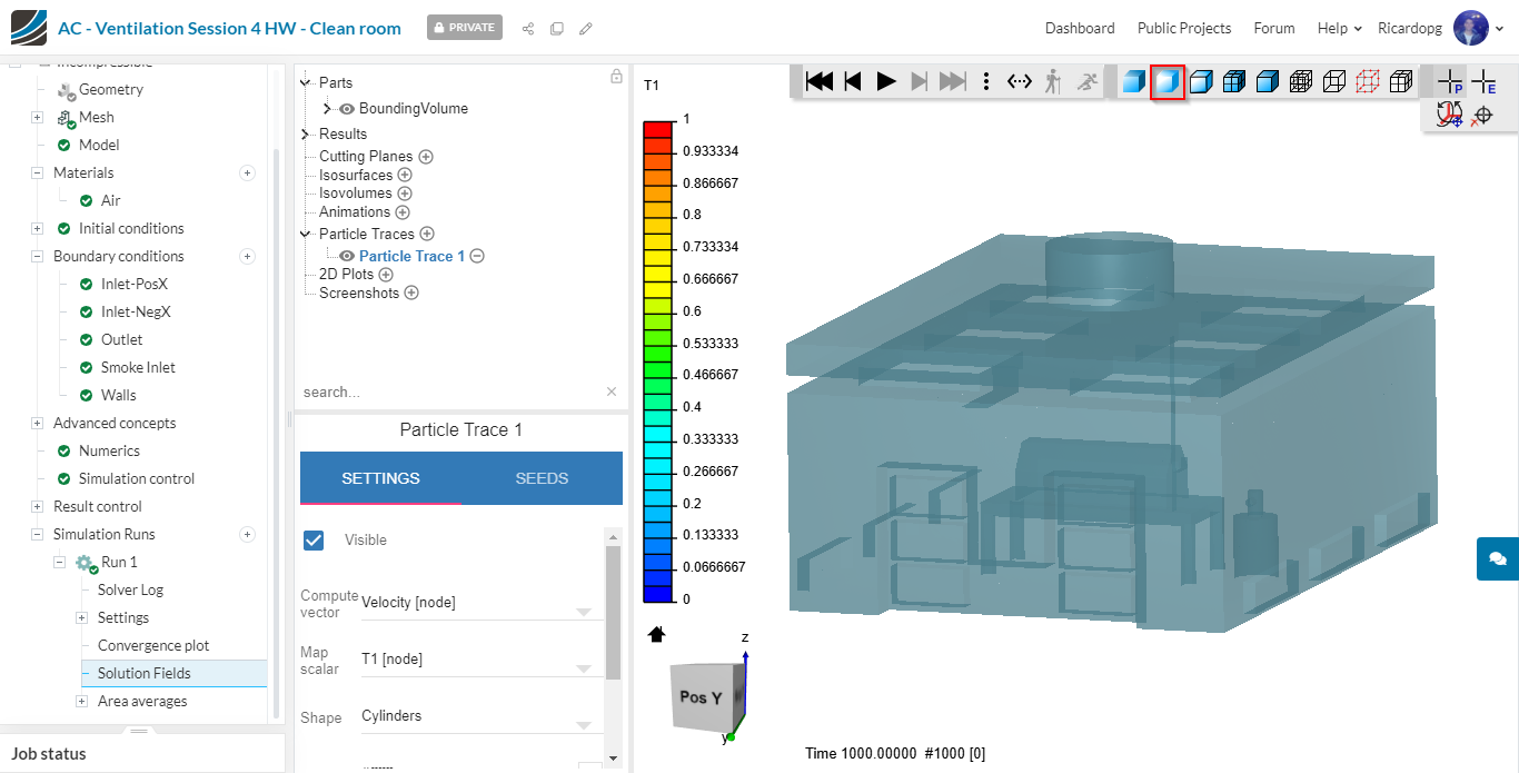
Stream lines are particularly useful to see how particles are flowing in the domain. You can assign stream lines by clicking on Particle Traces:

Towards the top right corner of the post-processing environment, you can find options for the surface representation. Please click on the Transparent Surface icon as shown below:
To set up the particle traces, click on SEEDS and then on PICK. Now click on a surface of your interest to generate stream lines. Usually the surfaces of interest are going to be inlets or outlets. In the picture below, one of the inlets was selected.
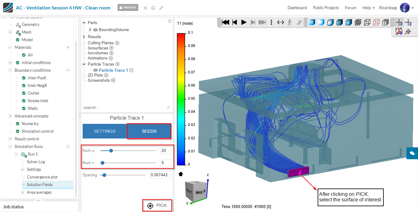
It’s possible to create multiple traces and assign them for different surfaces. 3 of the inlets are being analyzed in the picture below. The map color is based on the velocity of the particles: