Air Conditioning and Ventilation Webinar
Natural convection in a kitchen
Air Conditioning and Ventilation Workshop (Session 3) ― Heating of a Living Room
Import the project by clicking the link below (Ctrl+click to open in new tab).
Project Link: SimScale Login
Once the project is imported, the workbench is automatically opened. Then follow the steps below for setting up a convective heat transfer simulation.
Step-by-Step
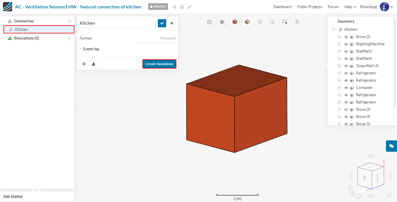
In the left-hand side panel, select the newly imported geometry Kitchen and click on Create Simulation.
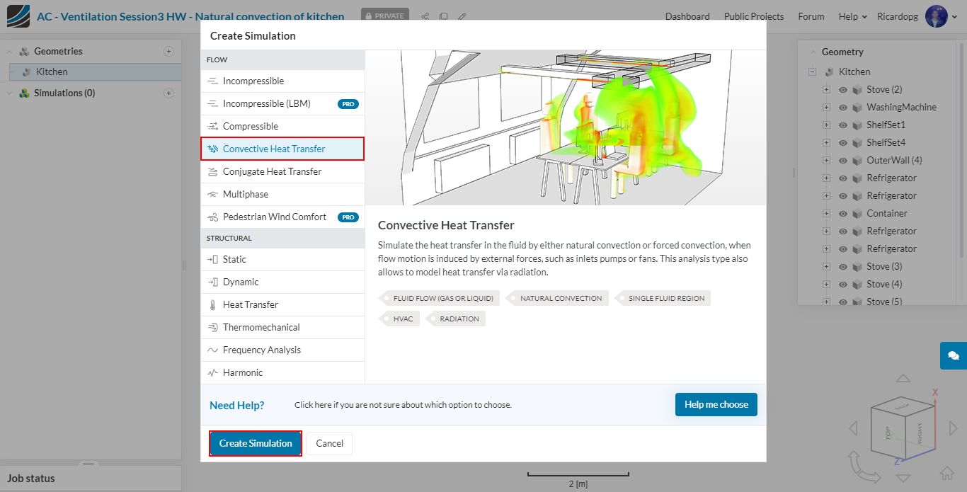
From the window that pops up, select Convective heat transfer as analysis type and proceed by clicking on Create Simulation:
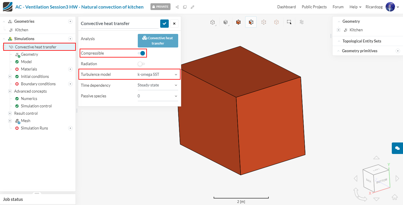
On the top of the tree, we can find some modeling options for our convective heat transfer analysis. For this one, we are going to use a k-omega SST Turbulence model and we are going to consider our fluid to be Compressible. Despite the fact that air is at low speeds, relatively small changes in temperature can produce relevant changes in density. Having the Compressible switch on means that we are not using the Boussinesq approximation.
The simulation tree is loaded on the left-hand side panel. Entries in red must be configured in order for us to run simulations.
Meshing
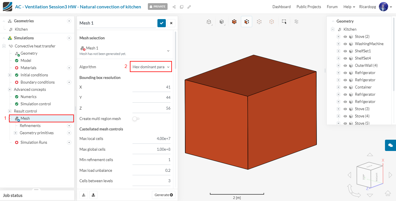
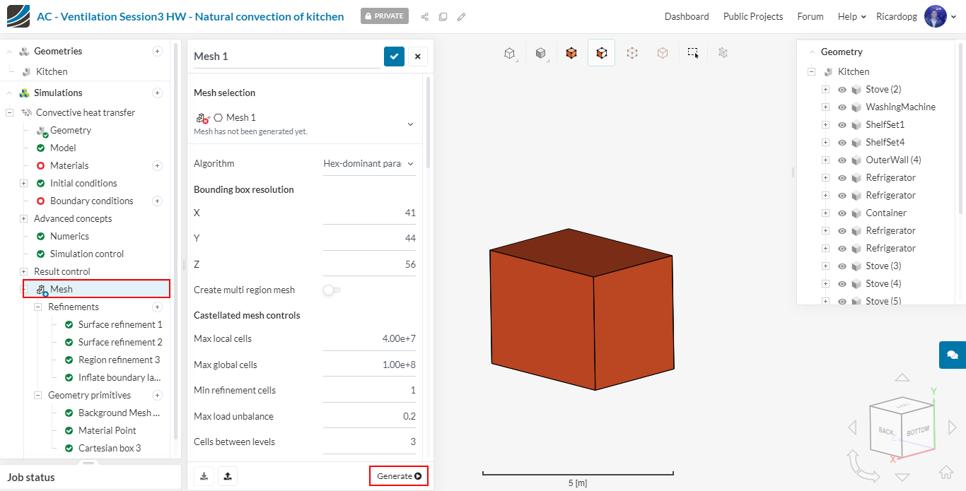
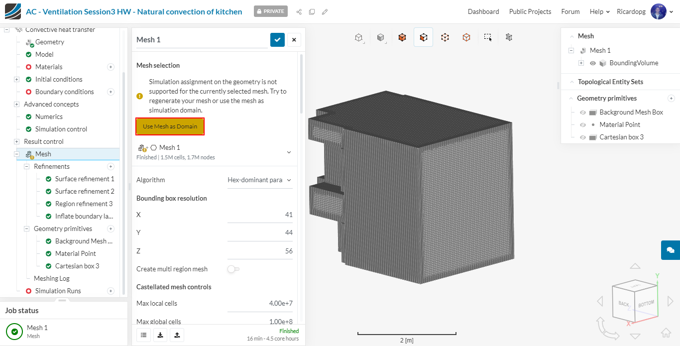
Having said that, please click on Mesh in the simulation tree. Change the Algorithm to Hex-dominant parametric (Only CFD).
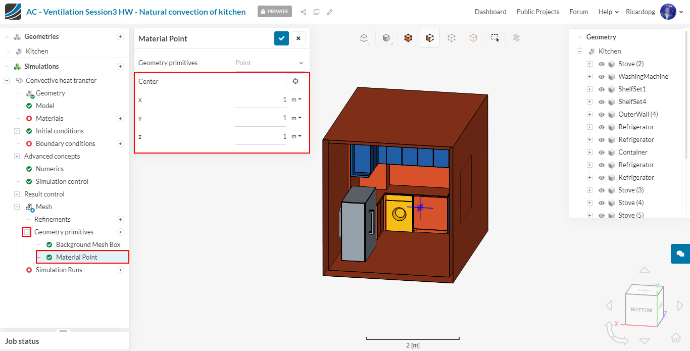
After changing the algorithm, a new simulation entry named Geometry primitives appears just under Mesh. Click on it to expand. Two primitives will be there by default: Background Mesh Box and Material Point.
Only Material Point has to be adjusted. You can place it anywhere inside the region that will be meshed (so, in this case, anywhere inside the kitchen room). For example, the coordinates (x, y, z) = (1, 1, 1) are good.
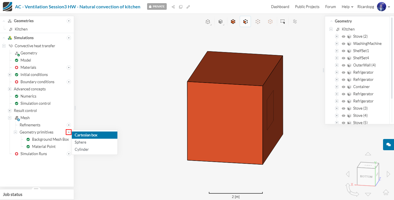
We will create a cartesian box geometry primitive. It will be used later on for a mesh refinement. To do that, click on the + icon next to Geometry primitives and select Cartesian box.
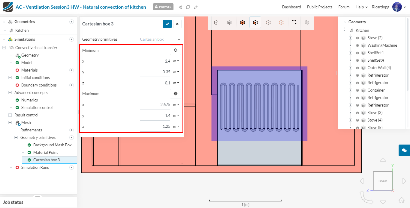
Input the following minimum and maximum coordinates (in meters):
Minimum: (2.4, 0.35, -0.1)
Maximum: (2.675, 1.4, 1.25)
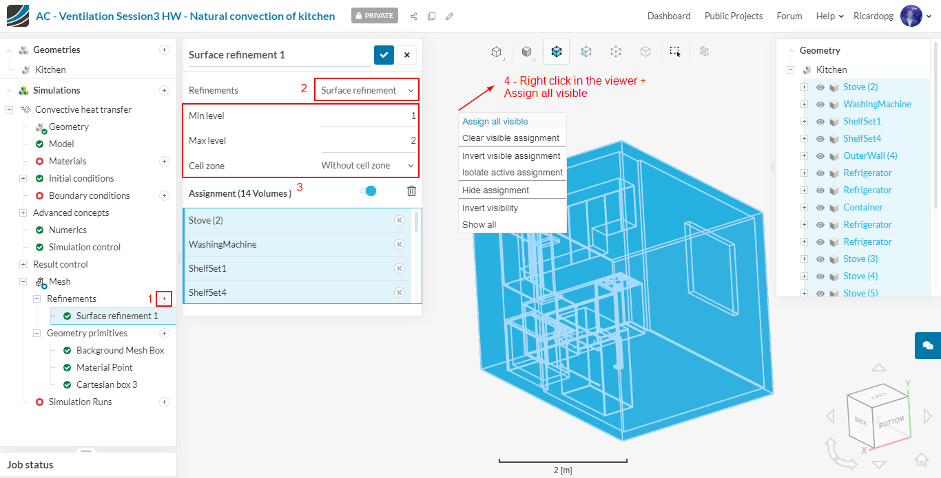
We will proceed to adding refinements now. Click on the + icon next to Refinements and select a Surface refinement. Assign all faces to this refinement. They will be refined from level 1 to 2.
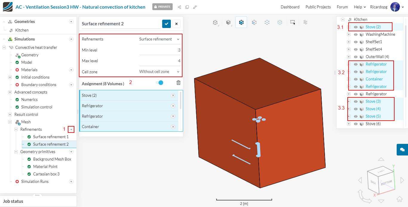
Make yet another Surface refinement. This time, Min level will be 3 and Max level will be set to 4. Use the right-hand side panel to select the 8 bodies shown below:
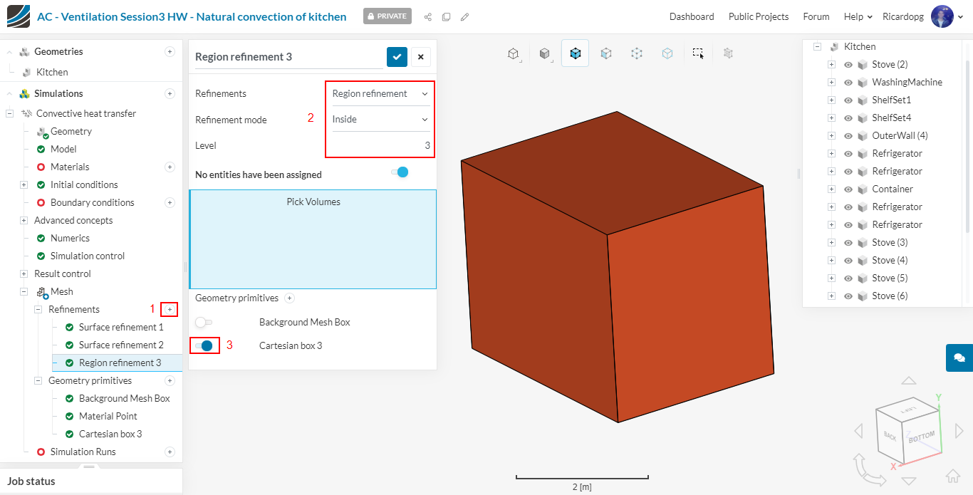
Using the previously created cartesian box, we will create a Region refinement. It will be used to get finer cells close to the heat source (refrigerator coils):
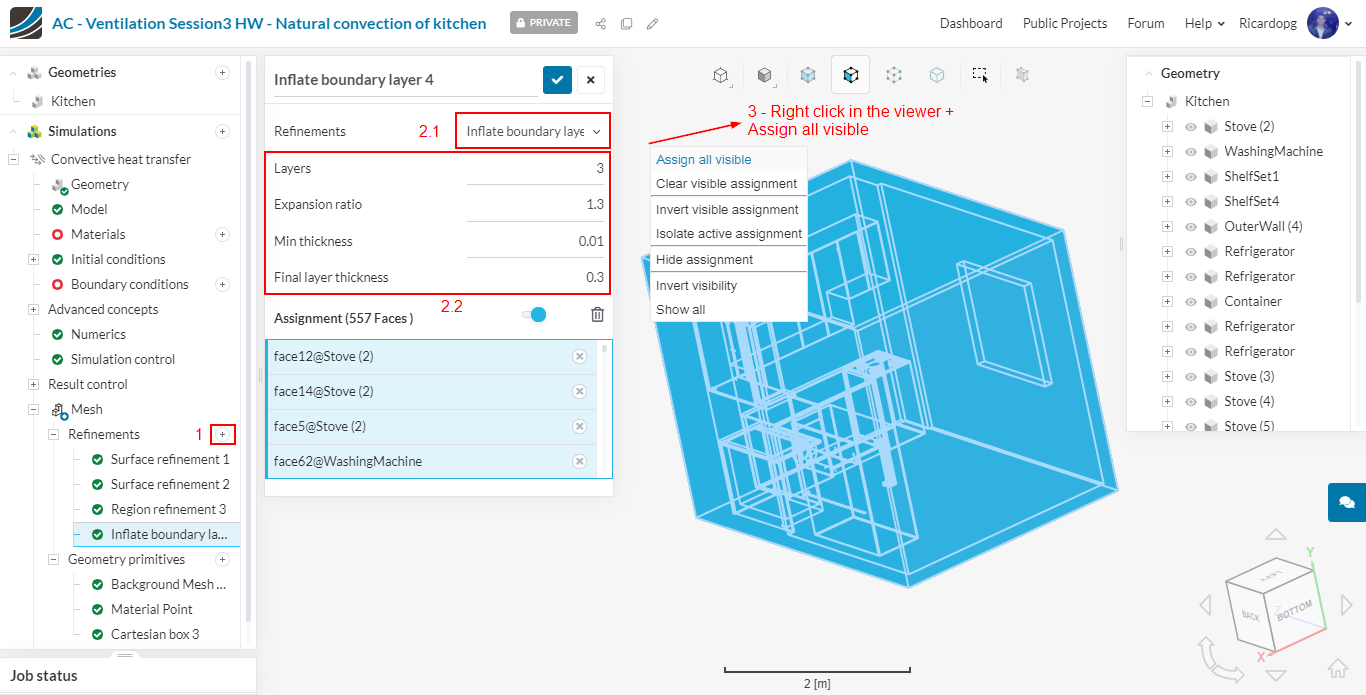
Lastly, an Inflate boundary layer refinement will be created to better capture the boundary layer profile. There will be 3 Layers with a 1.3 Expansion ratio. Min thickness and Final layer thickness are 0.01 and 0.3 respectively.
Now please go back to Mesh and run the operation by clicking on Generate. The number of processors is chosen automatically to optimize core hours usage.
The meshing operation takes about 16 minutes to finish. Once the mesh is ready, make sure to click on Use Mesh as Domain.
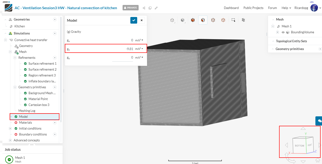
We can configure the rest of the entries now. First, starting with Model, please input -9.81 m/s² as gravity in the y direction.
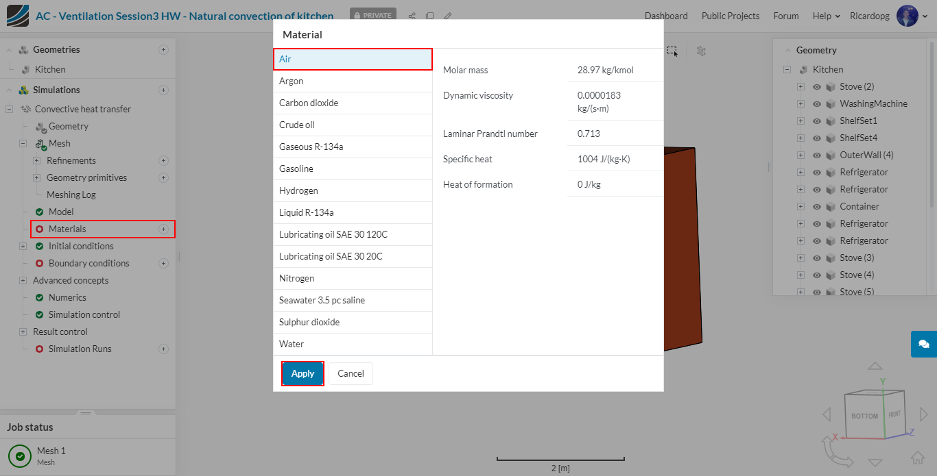
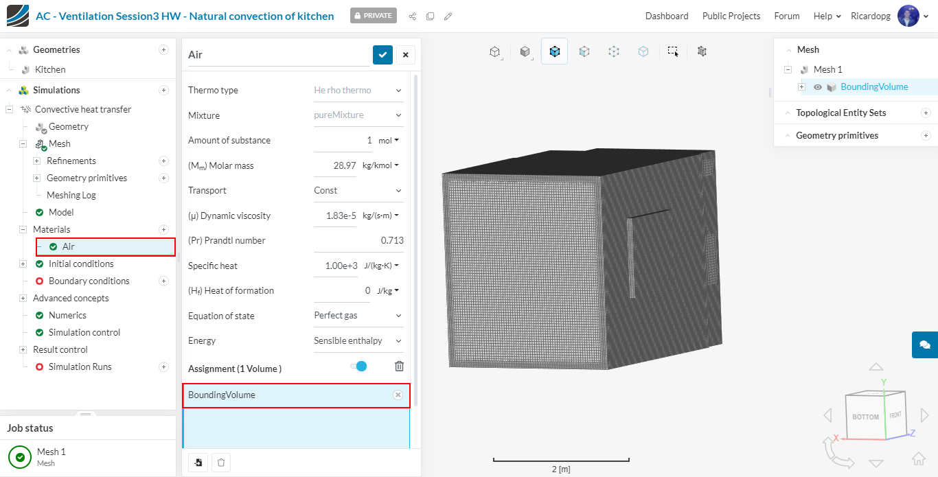
In Materials, select Air and click on Apply. It will be automatically assigned to the flow region.
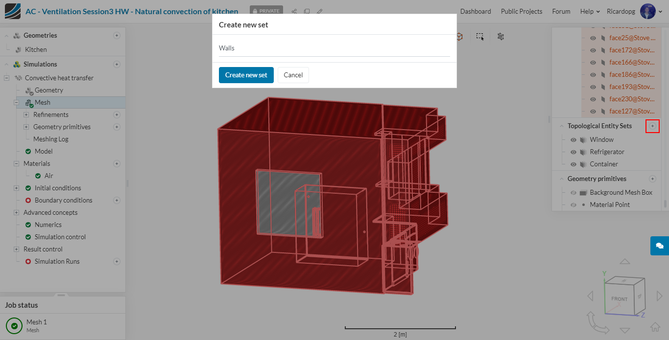
Topological Entity Sets can help us to quickly select different sets of faces. It’s particularly useful when creating boundary conditions.
To create one entity set, select the face or faces that will be grouped together, then click on the + icon next to Topological Entity Sets in the right-hand side panel. Finally name the group as you find appropriate.
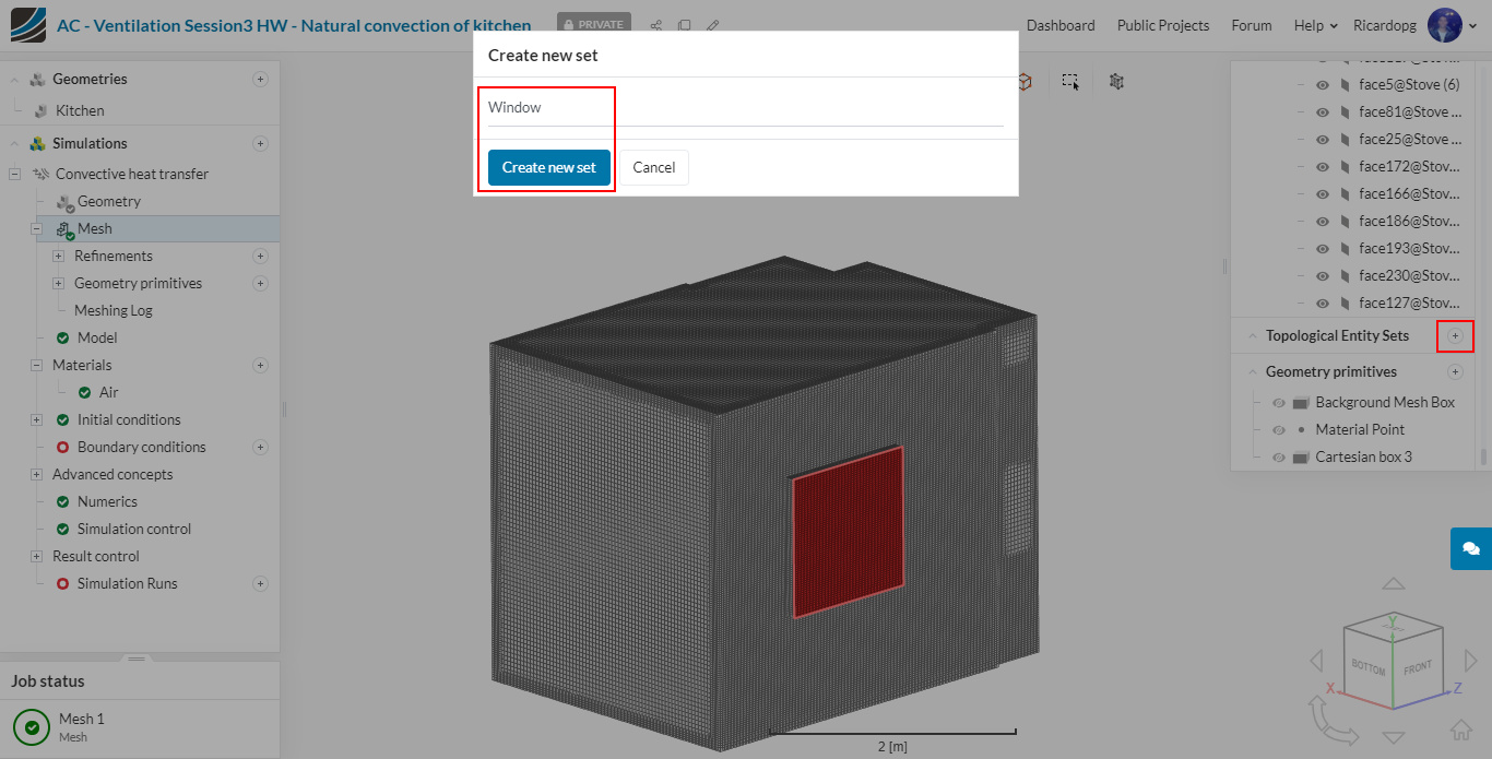
For instance, to create a Window topological entity set, do as follows:
1- Select the face that represents the window:

2 - Create a new set by adding a topological entity set and renaming it:
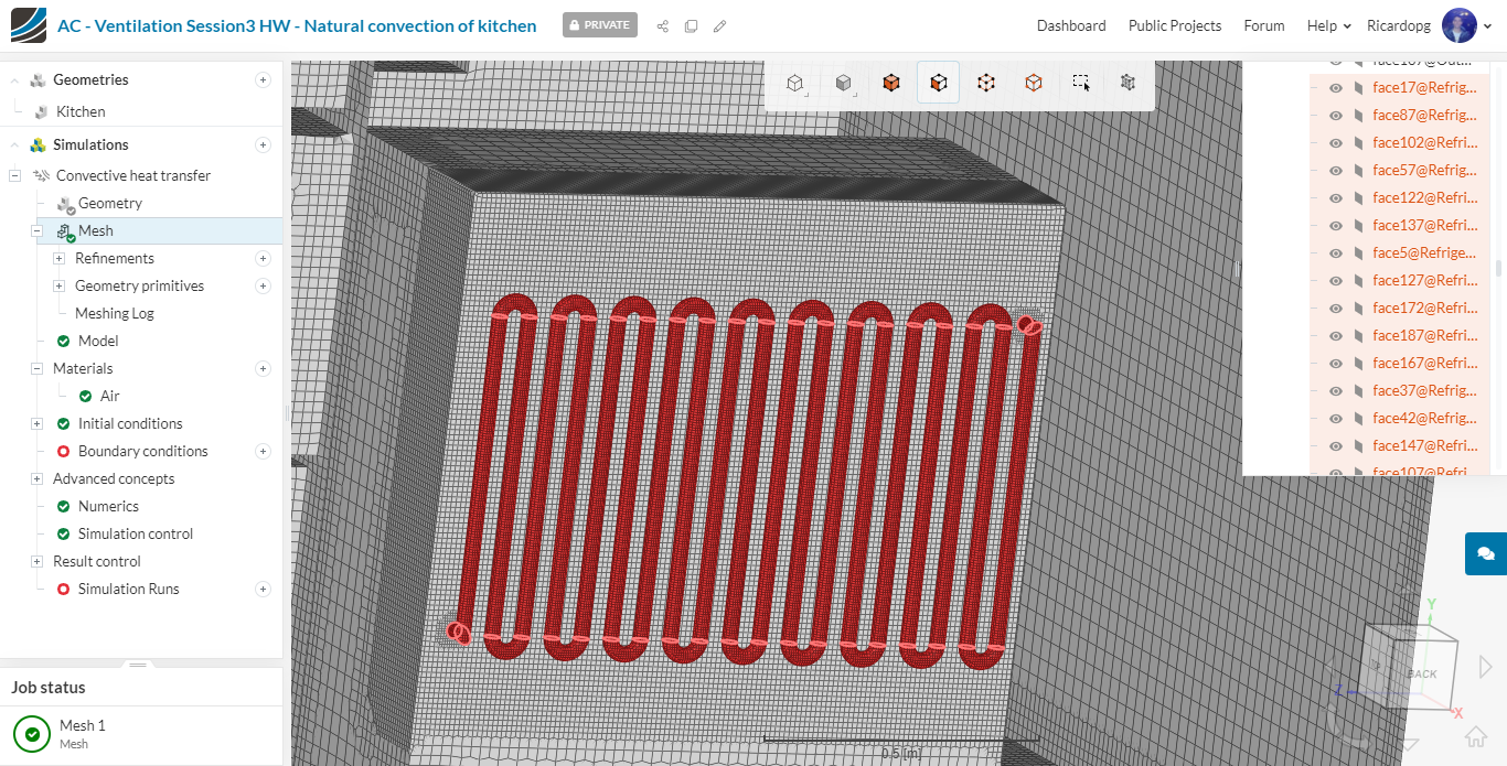
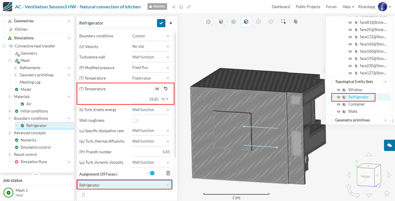
The selection of refrigerator coil needs to be done manually. To visualize the coils, first hide one of the external walls:
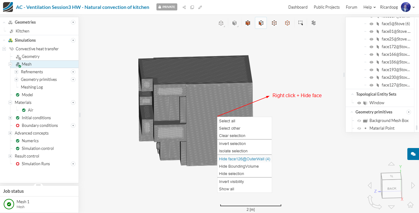
Then manually select all the coils behind the refrigerator and create a Refrigerator topological entity set.
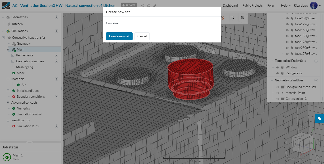
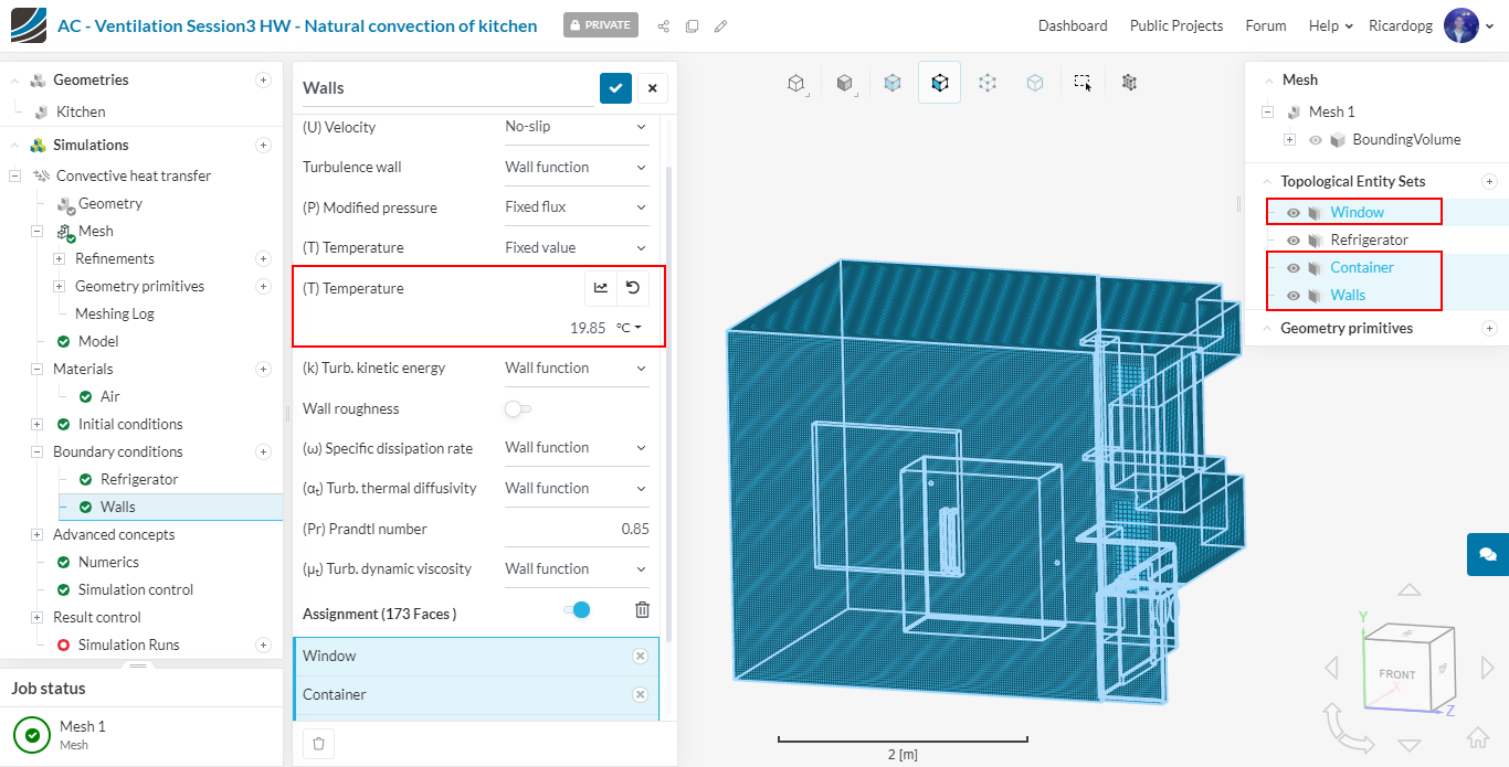
Now, on top of the oven, there will be a container, consisting of 4 faces in total. Please select all of them and create a Container topological entity set:
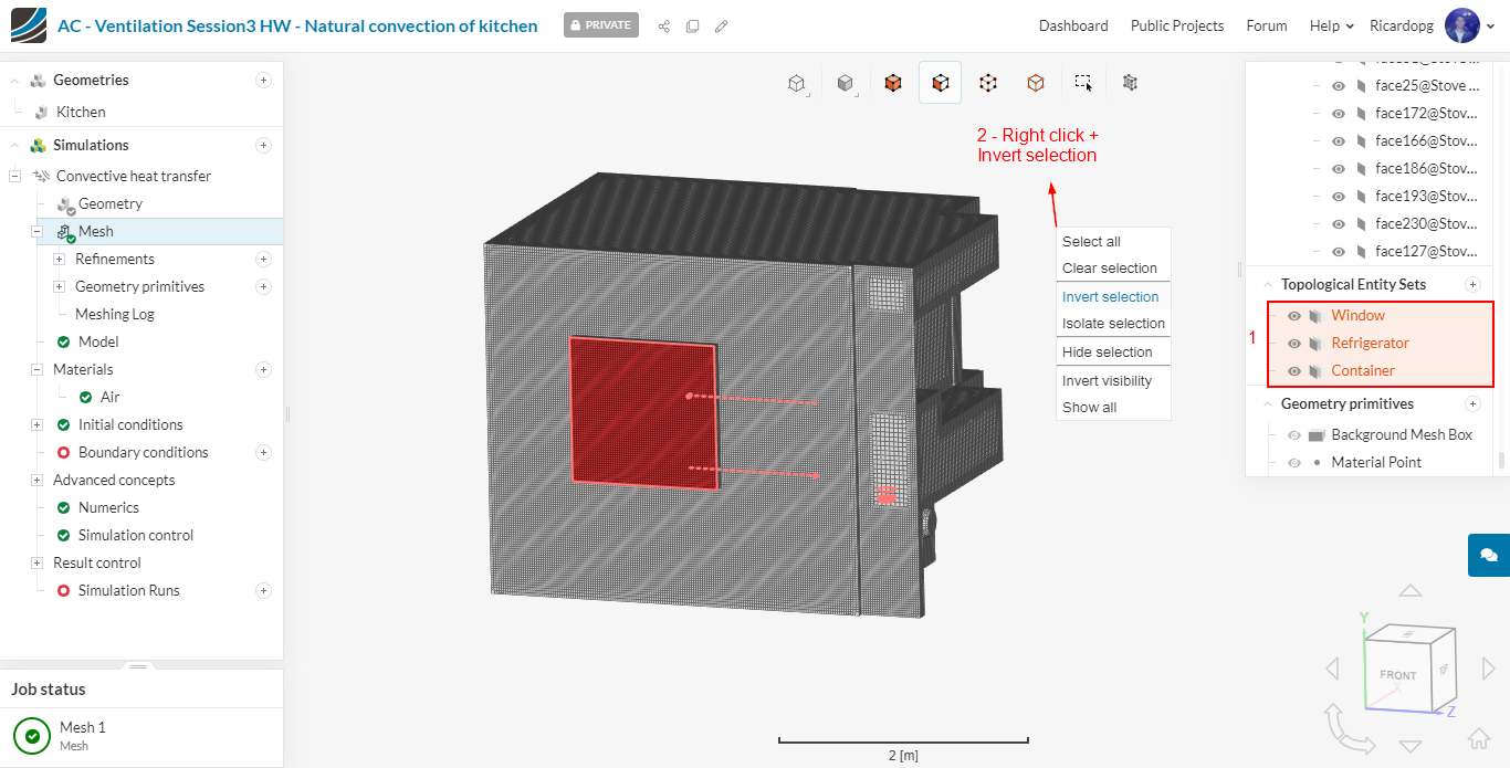
The last topological entity set will be called Walls. To avoid having to manually select all walls, simply select all previously created entity sets, then right click in the viewer and Invert selection:
Boundary conditions
Initial conditions will remain as default. We will use the previously created topological entity sets to create the boundary conditions. For this project, 3 different configurations will be explored. This step-by-step shows how to configure the first one:
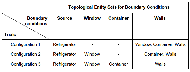
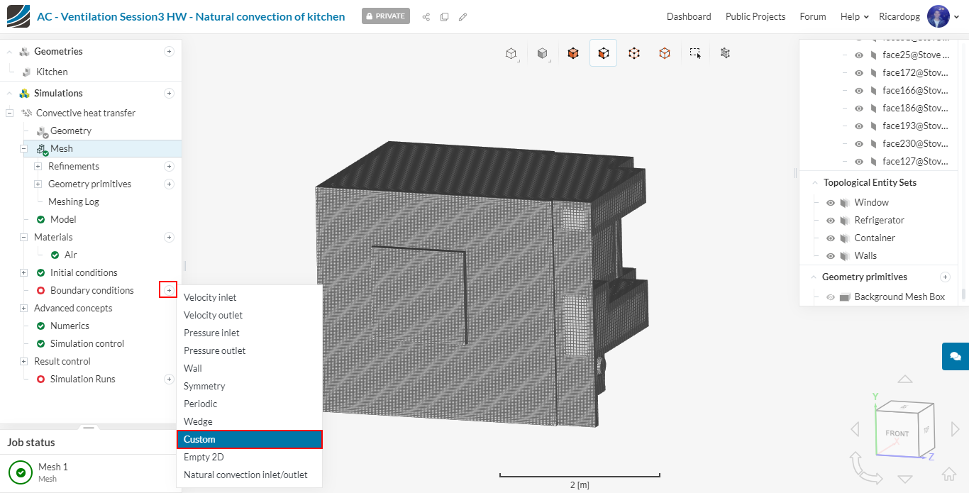
The Source boundary condition is created as follows:
The Walls boundary condition is also custom. It has the same settings as the source boundary condition previously created, except for the temperature value. Walls will have a fixed temperature of 19.85 Celsius. Assign it to the following entity sets: Walls, Container and Window:
NOTE: for configurations 2 and 3: Window and Container boundary conditions are the same as Walls, only their temperatures are different. For Window, temperature will be fixed at 9.85 Celsius, whereas Container will have its temperature fixed at 49.85 Celsius.
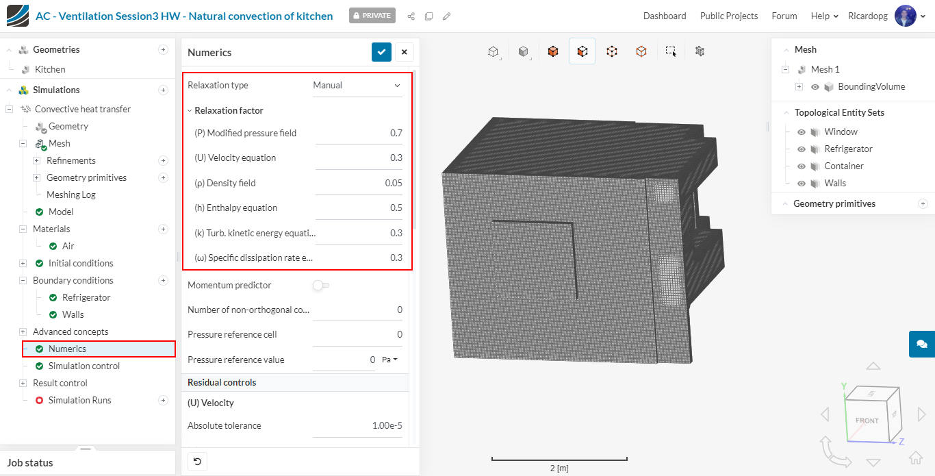
Heading over to Numerics, there are a few changes to be made. Set Relaxation type to Manual and input the following:
( P) Modified pressure field: 0.7;
(U) Velocity equation: 0.3;
(ρ) Density field: 0.05;
(h) Enthalpy equation: 0.5;
(k) Turb. kinetic energy equation: 0.3;
(ω) Specific dissipation rate equation: 0.3.
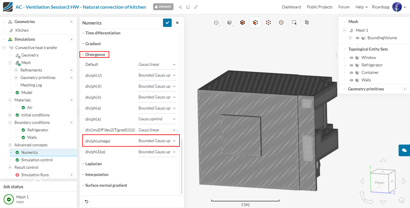
Scrolling further down on Numerics, find Divergence schemes. Change div(phi,omega) to Bounded Gauss Upwind:
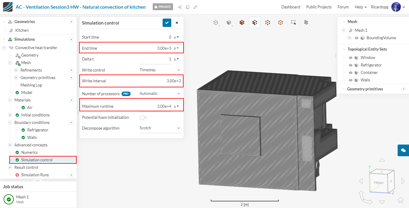
In Simulation control, change End time and Write interval to 3000 iterations. Also change Maximum runtime to 30000 seconds.
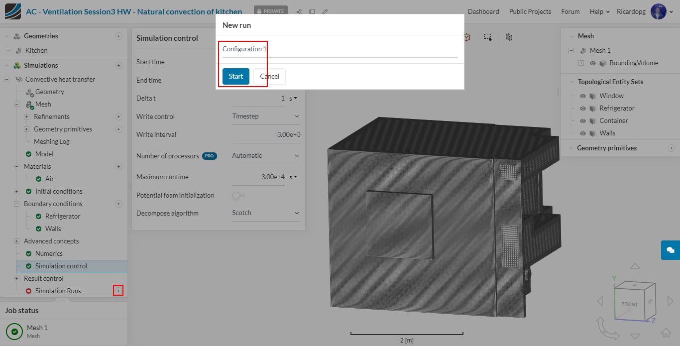
That’s it for configuration 1. Proceed to Simulation Runs, name it Configuration 1 and hit Start.
To make it easier to setup configurations 2 and 3, make sure to duplicate the first simulation. Then only few boundary condition adjustments will be needed.
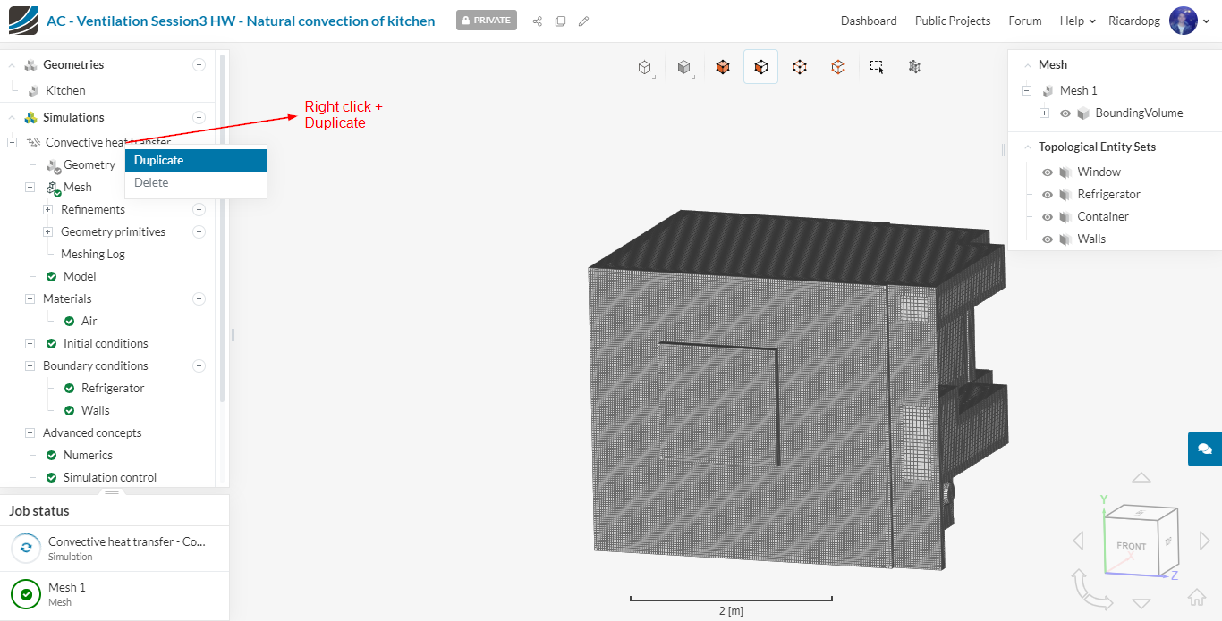
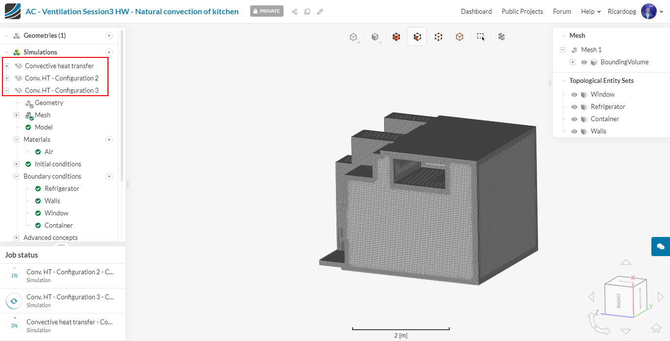
You can even run all 3 simulations at the same time. SimScale allows running multiple jobs in parallel.
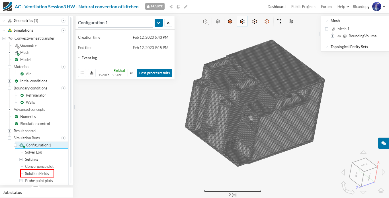
Post-processing
When the runs are finished, click on Solution Fields to access the post-processing environment.
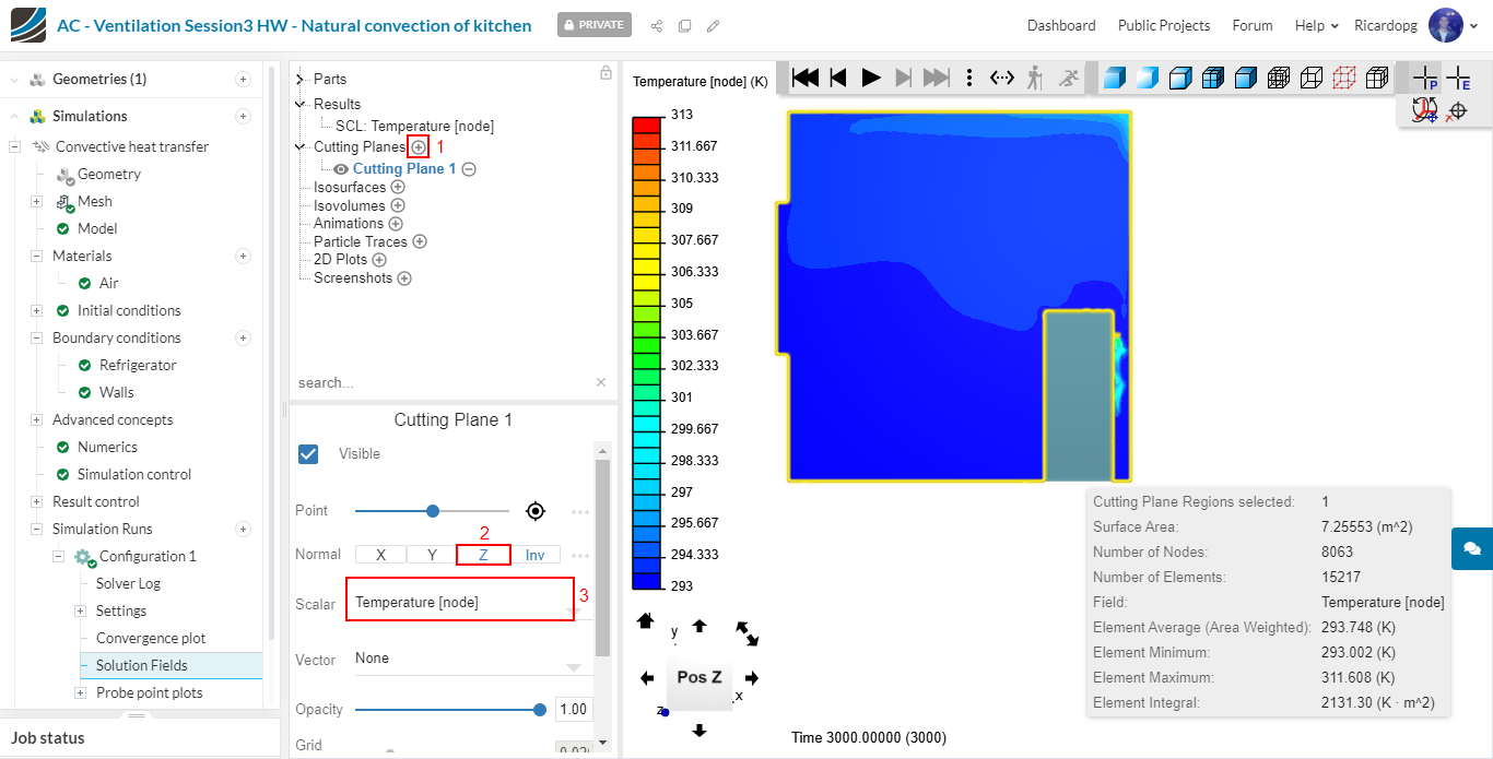
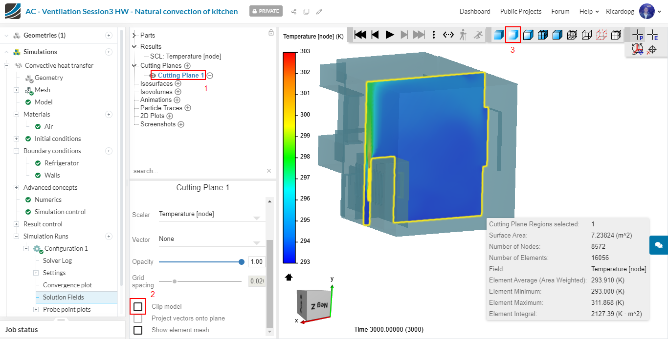
Let’s add a Cutting Plane to slice the geometry,
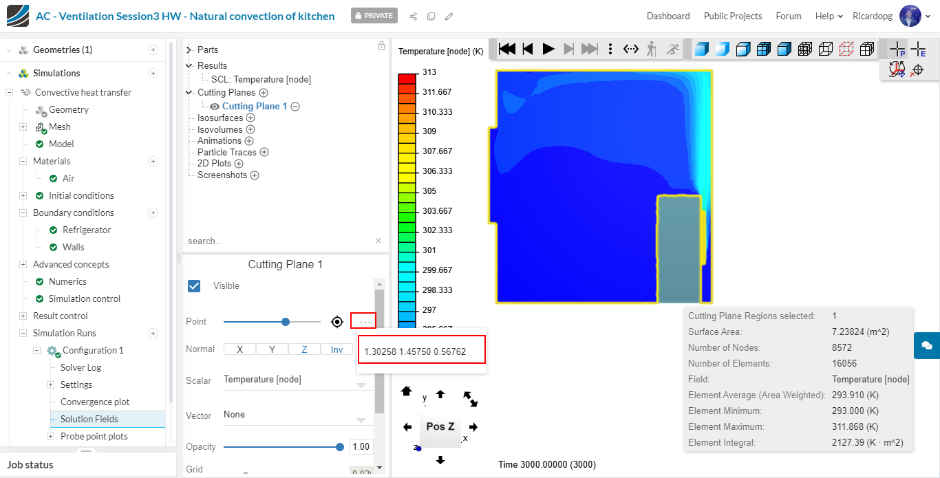
Next to Point, there will be three dots. Click on them and specify the following coordinates for the cutting plane origin: (1.30258, 1.45750, 0.56762).
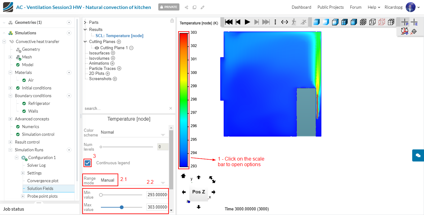
Adjust the scale bar’s range to 293 - 303 K:
It might be interesting to display the domain as well for better visualization. This can be done by unselecting Clip model and then making the surfaces semitransparent.
Click on the “eye” next to the cutting plane that you created to hide it. We will now create an Isovolume. The isovolume is a volumetric representation of a certain property in a determined range. For instance, select Temperature [node] for both Iso scalar and Map scalar. Adjust the range from 300 to 313 K:
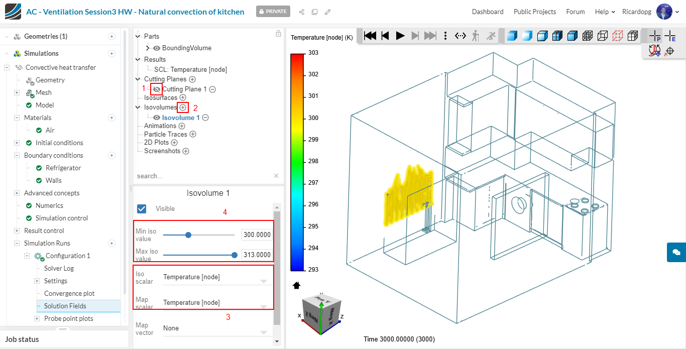
All the highlighted volume in the viewer is within this temperature range.
Try widening the range to 295 - 313 K:
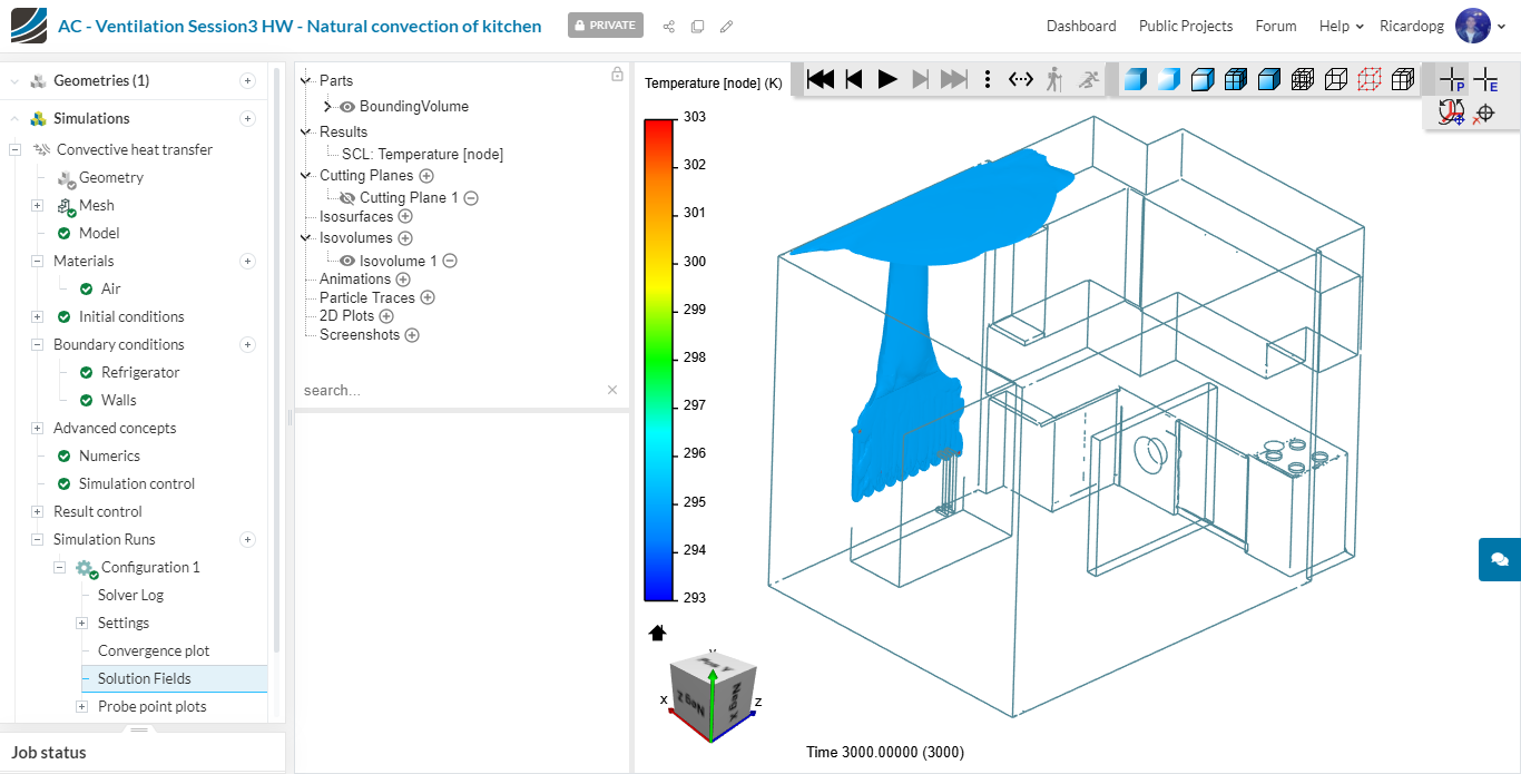
Do a similar post-processing to the other configurations and compare the results!