Homework Assignment for Air-Conditioning and Ventilation webinar: Session-2
Air Conditioning and Ventilation Workshop (Session 2) ― Smoke Propagation in Garage
Step-by-Step
Import the project by clicking the link below:
Project Link: SimScale Login
Once the project is imported, the workbench is automatically opened.
Then follow the steps below for setting up a Steady-state Turbulent Scalar Transport analysis to simulate the smoke propagation in an indoor parking garage.
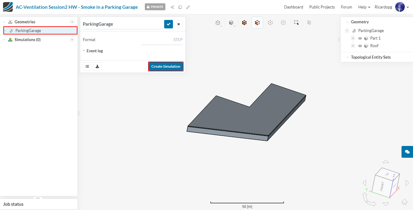
The first step is to click on the ParkingGarage geometry and select Create Simulation.
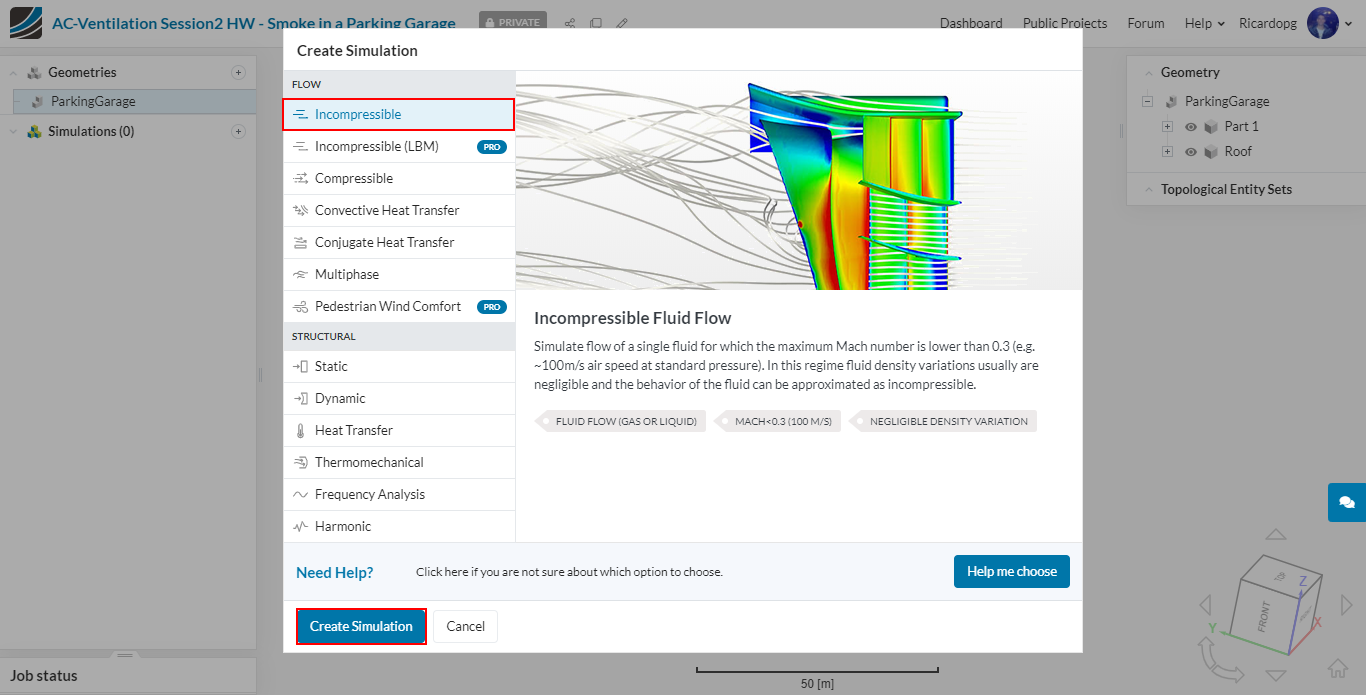
In the window that opens up, select Incompressible and click on Create Simulation one more time.
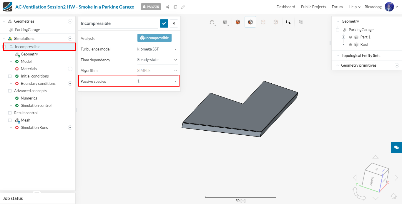
The smoke is going to be modeled as a passive scalar. So, in the Incompressible tab, make sure to change the number of Passive species to 1.
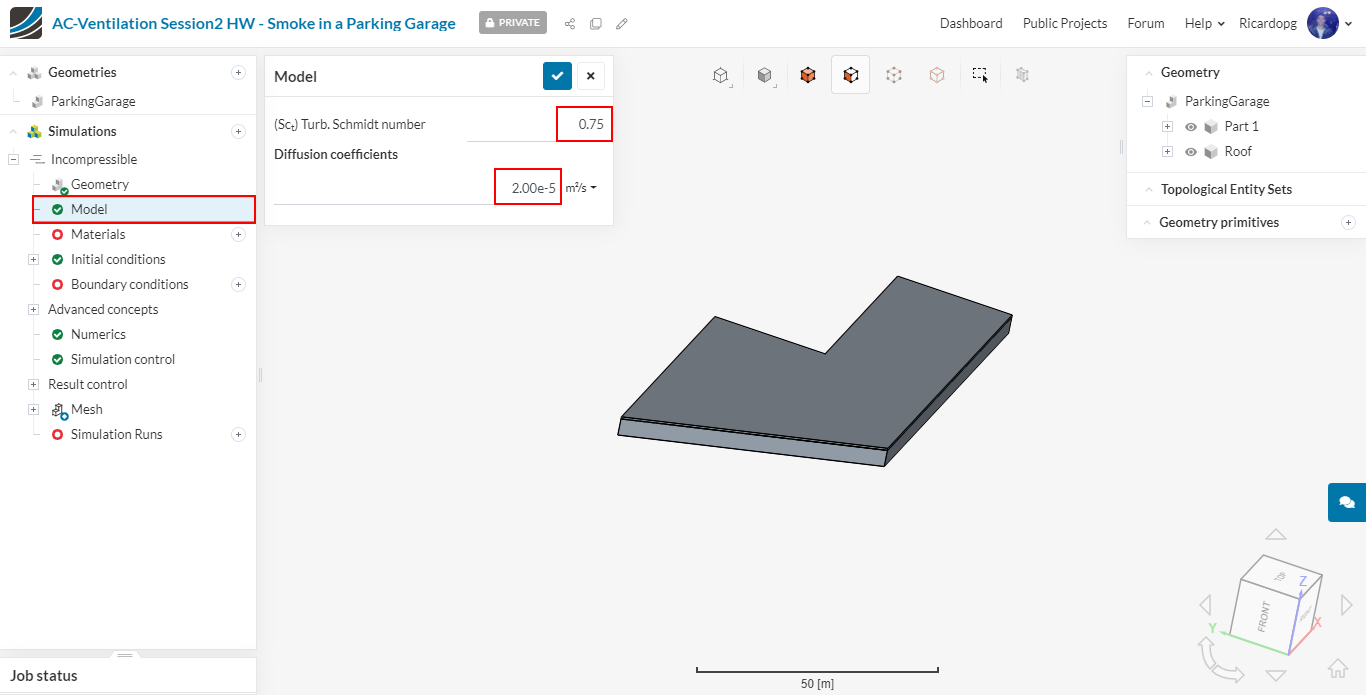
The passive scalar will spread through the flow region by means of convection and diffusion. In Model , we can assign a Diffusion coefficient . This coefficient is usually given for a binary of materials (e.g. air and CO). The coefficient for some binary gas mixtures can be found here.
In our case, please assign it a value of 0.00002 {m² \over s}. Also change Turb. Schmidt number to 0.75.
Mesh
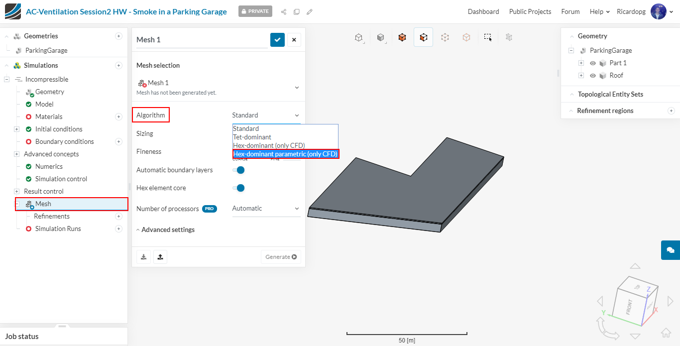
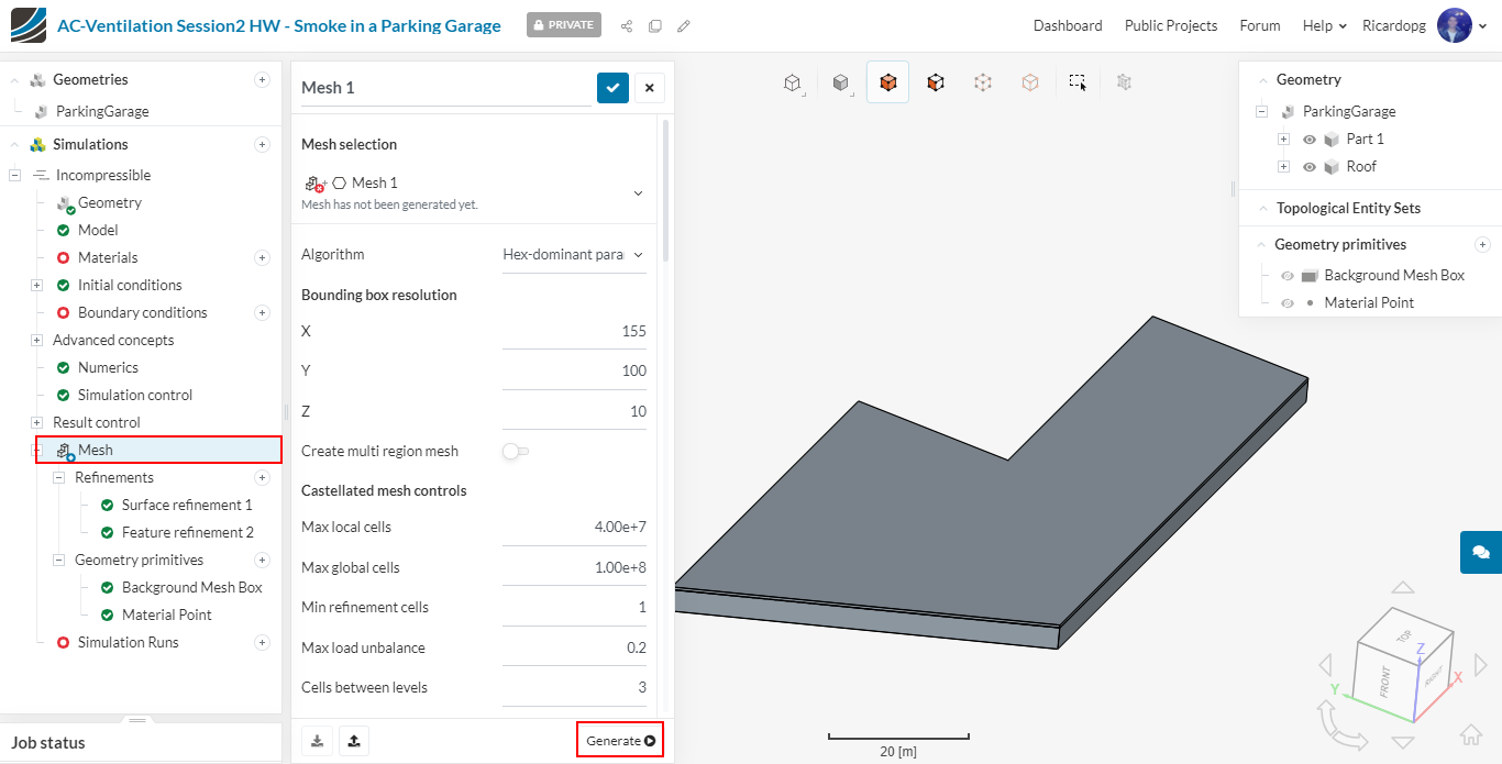
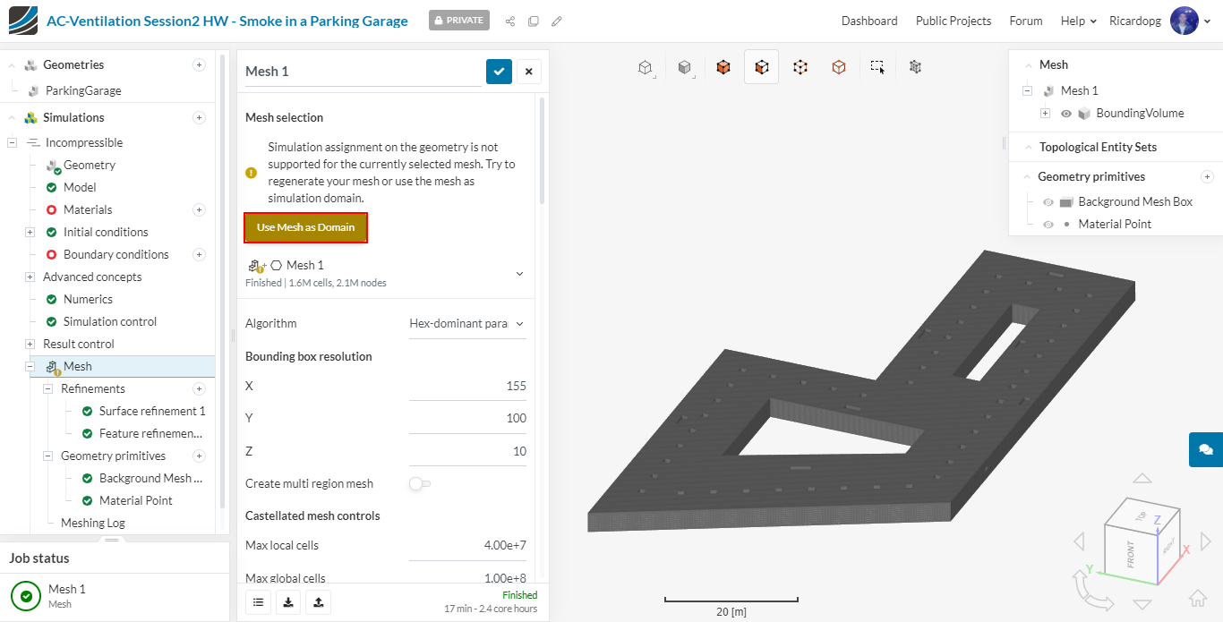
In the simulation tree, navigate to Mesh. Change the Algorithm to Hex-dominant parametric (only CFD).
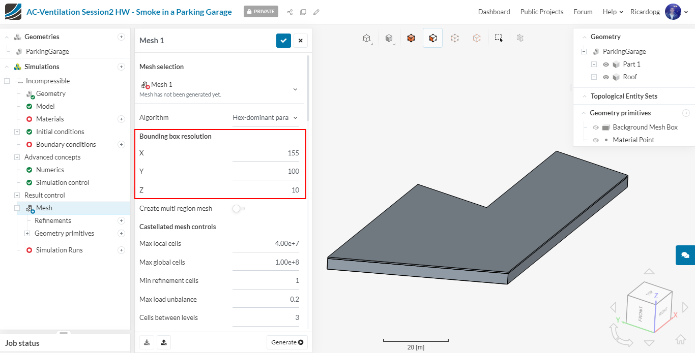
In Bounding box resolution, please input the following:
- 155 cells in the X direction;
- 100 cells in the Y direction;
- 10 cells in the Z direction.
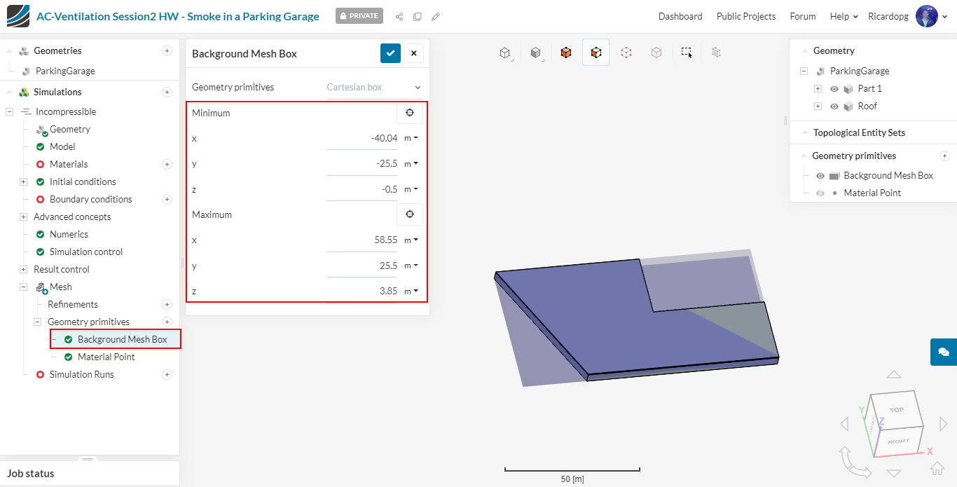
Under Mesh, please expand Geometry primitives. Click on Background Mesh Box and input the following coordinates:
- x minimum: -40.0384 m
- y minimum: -25.5 m
- z minimum: -0.5 m
- x maximum: 58.5514 m
- y maximum: 25.5 m
- z maximum: 3.85 m
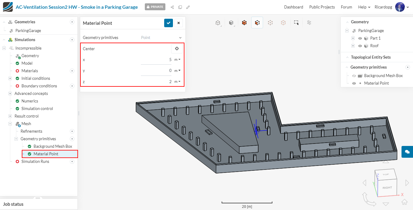
Just under Background Mesh Box, you will find Material Point. Please adjust the coordinates to 5 in the x direction, 0 in the y direction and 2 in the z direction.
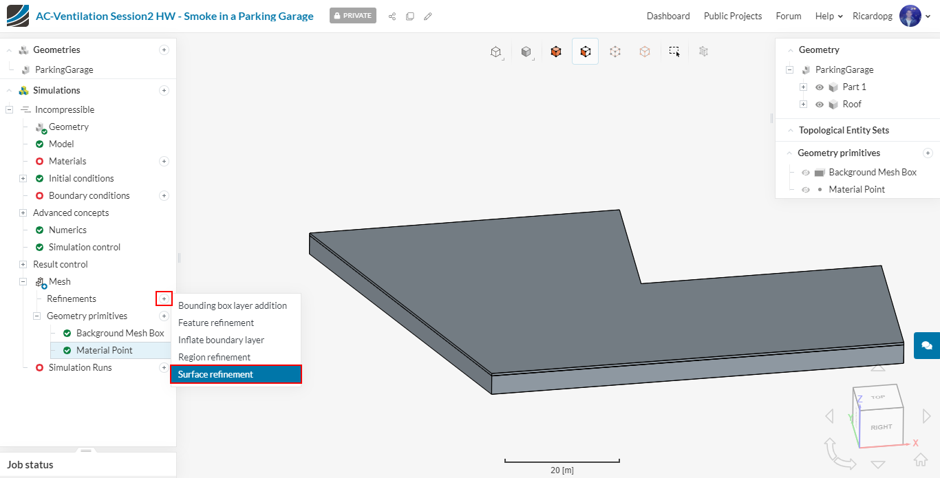
Let’s now assign mesh Refinements to refine the mesh in critical areas. Please click on the + icon next to Refinements and select a Surface refinement:
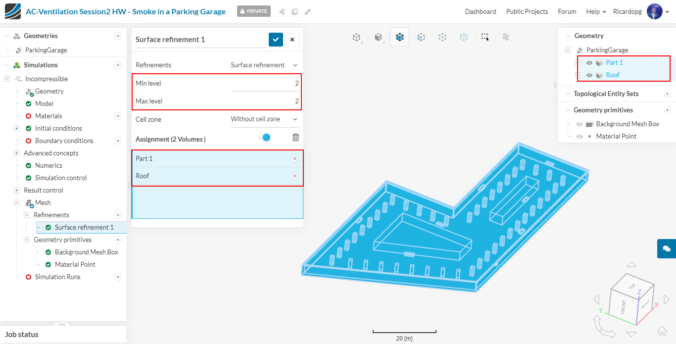
Set both Min level and Max level to 2 and assign this refinement to Roof and Part 1 by clicking in these parts in the right-hand side panel:
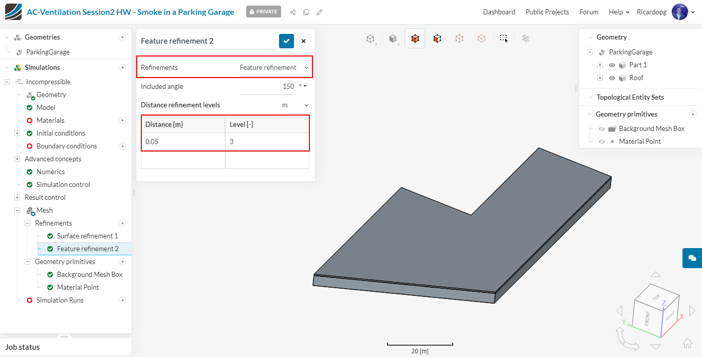
Please create a new Refinement, this time a Feature refinement.
Head back to Mesh and start the meshing operation by clicking on Generate. You don’t have to worry with the number of processors that will be employed. SimScale automatically determines the number of processors based on the job size.
The mesh takes about 17 minutes to finish. Once the operation is over, make sure to click on Use Mesh as Domain.
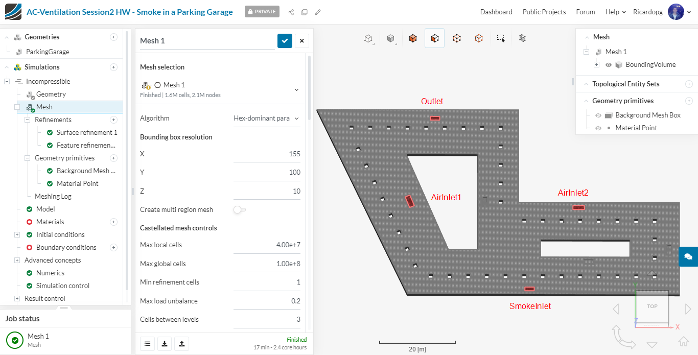
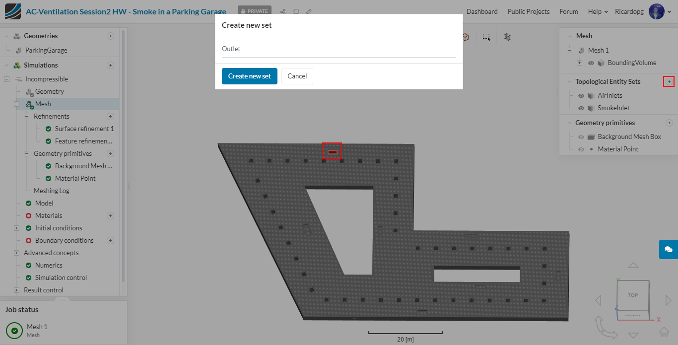
Now let’s proceed to creating Topological Entity Sets. To create one set, select the face or faces that will be grouped together, then click on the + icon next to Topological Entity Sets in the right-hand side panel. Finally name the group as you find appropriate.
Let’s create topological entity sets for AirInlets, SmokeInlet, Outlet and Walls. Please refer to the following picture when creating the sets.
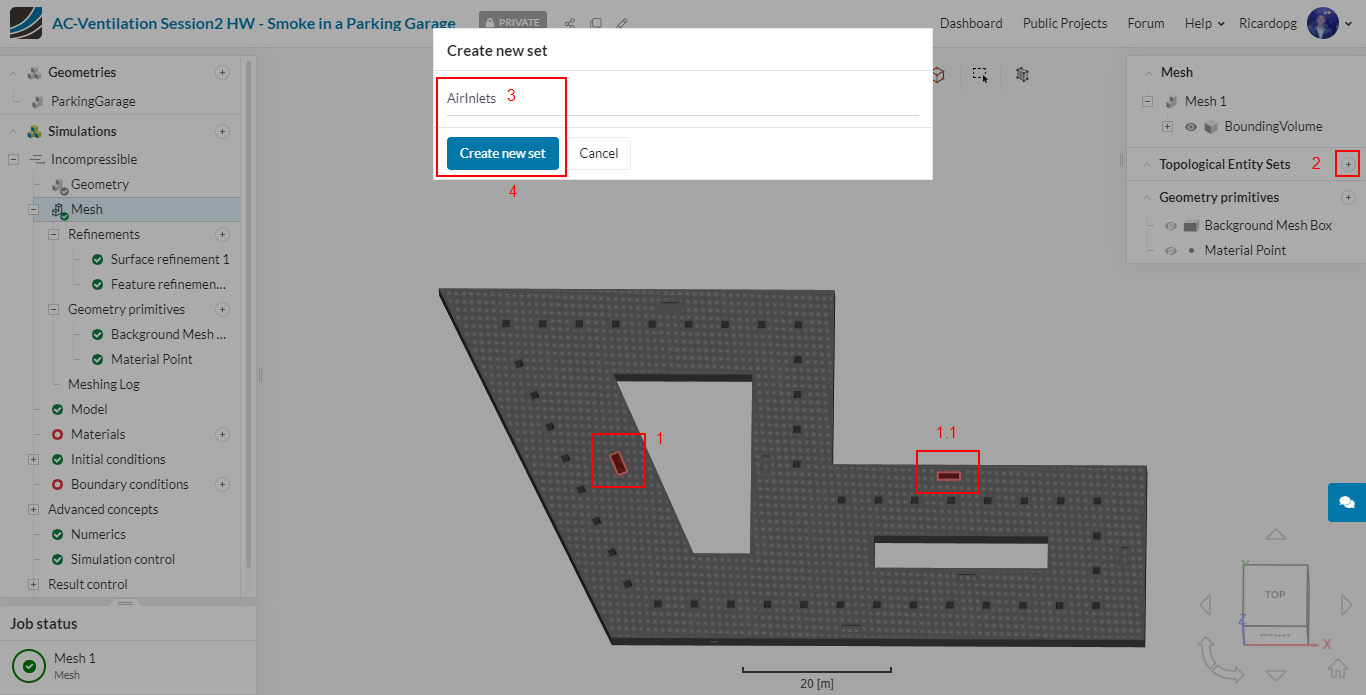
So, to create the AirInlets set, the user should follow these steps:
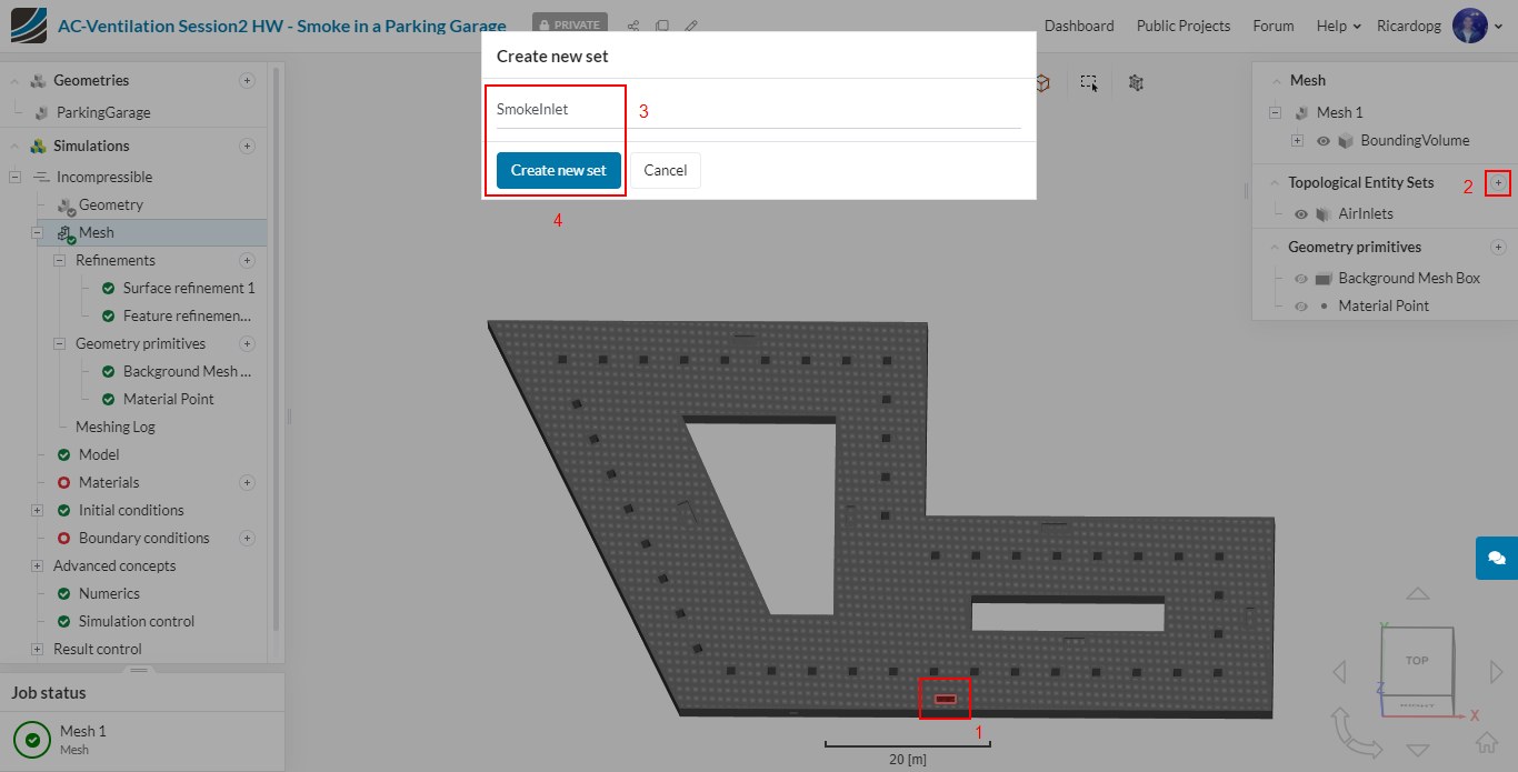
Similarly, for the SmokeInlet set:
To create the Outlet set:
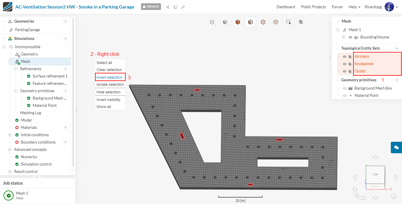
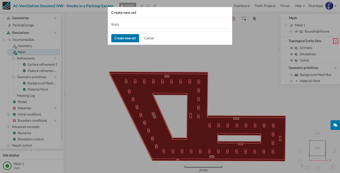
And finally, to create the Walls set, simply select all the sets previously created, then right click in the viewer to Invert selection. All walls will be assigned and the set can be easily created:
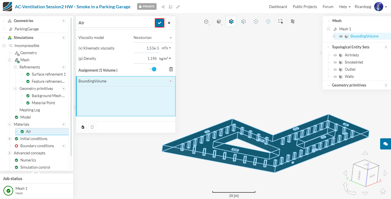
Let’s now assign a material to our flow region. In the simulation tree, navigate to Materials. Select Air from the materials library and hit Apply.

The BoundingVolume will be automatically assigned, so simply click on the blue mark to save.
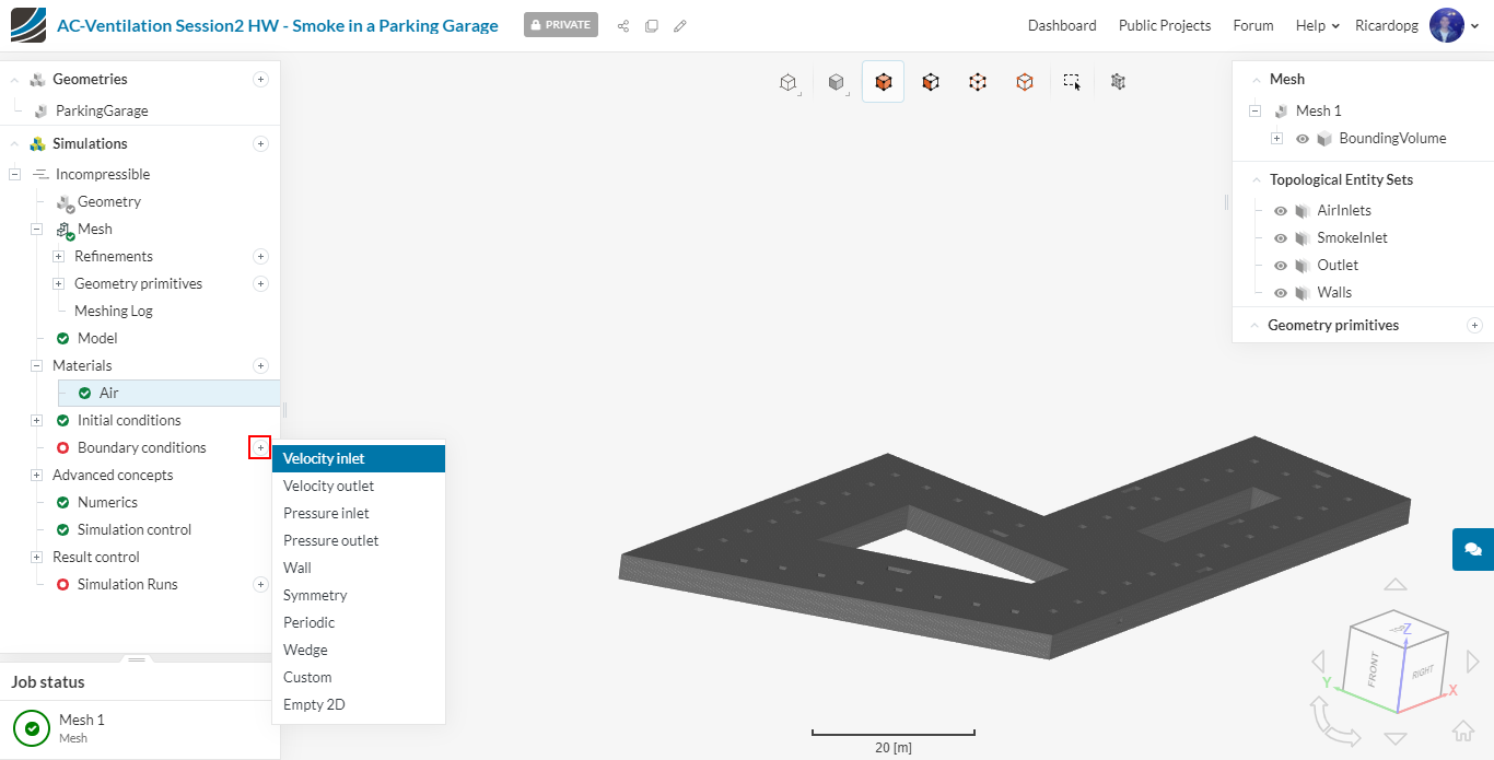
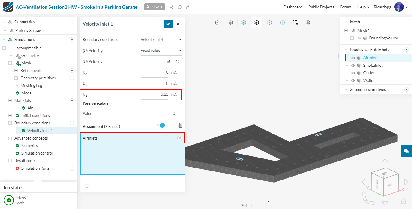
Let’s now assign the Boundary conditions. For the first one, select a Velocity Inlet boundary condition:
Set it up as shown below. Value 0 for Passive scalars indicates fresh air:
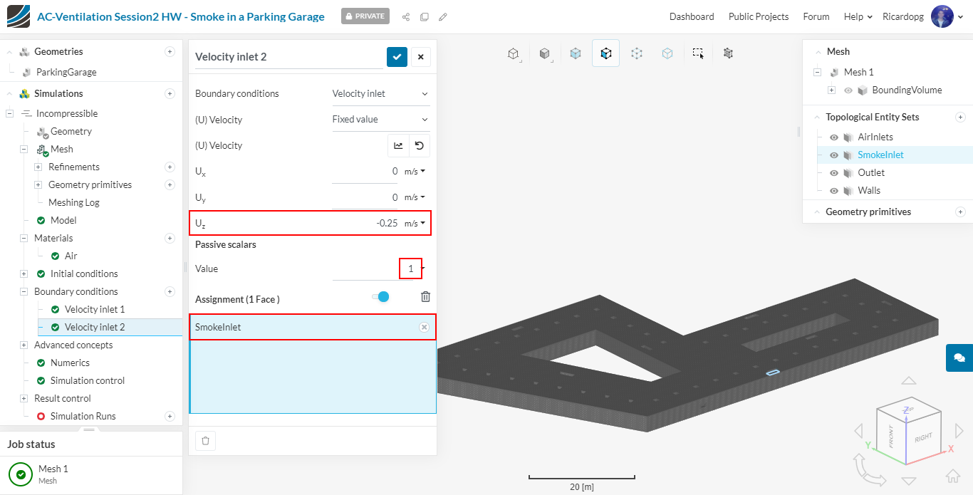
Now select another Velocity Inlet boundary condition, this time for the SmokeInlet:
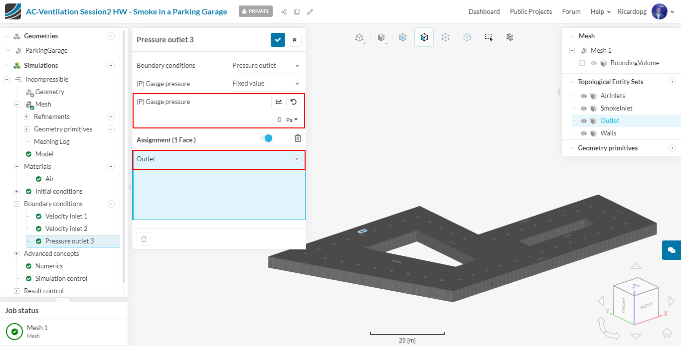
The Outlet patch will have a Pressure outlet boundary condition applied to it:
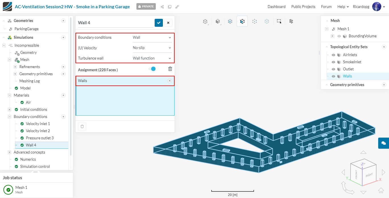
And Walls will have a simple Wall boundary condition, with a No-slip condition for velocity and Wall function for wall treatment:
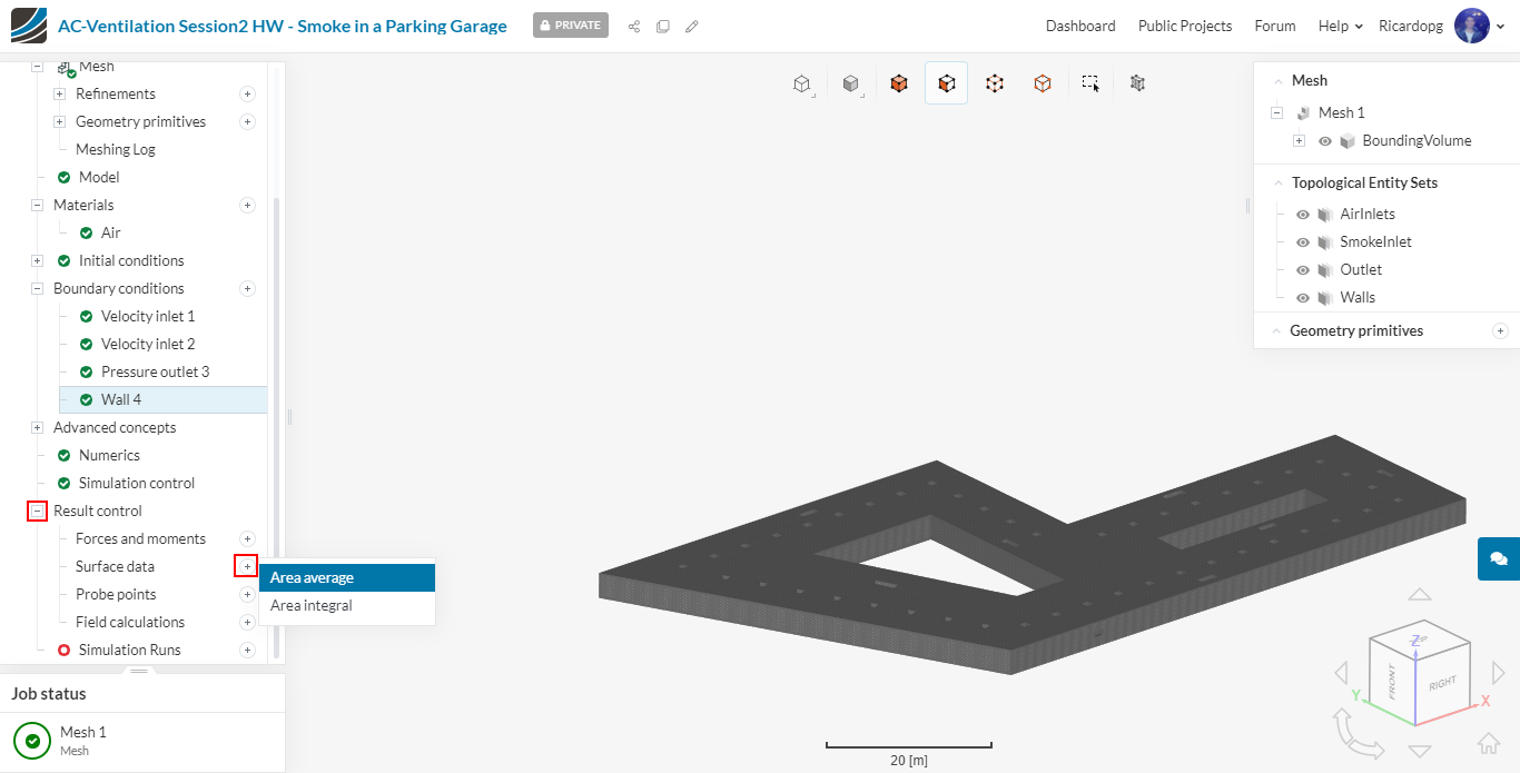
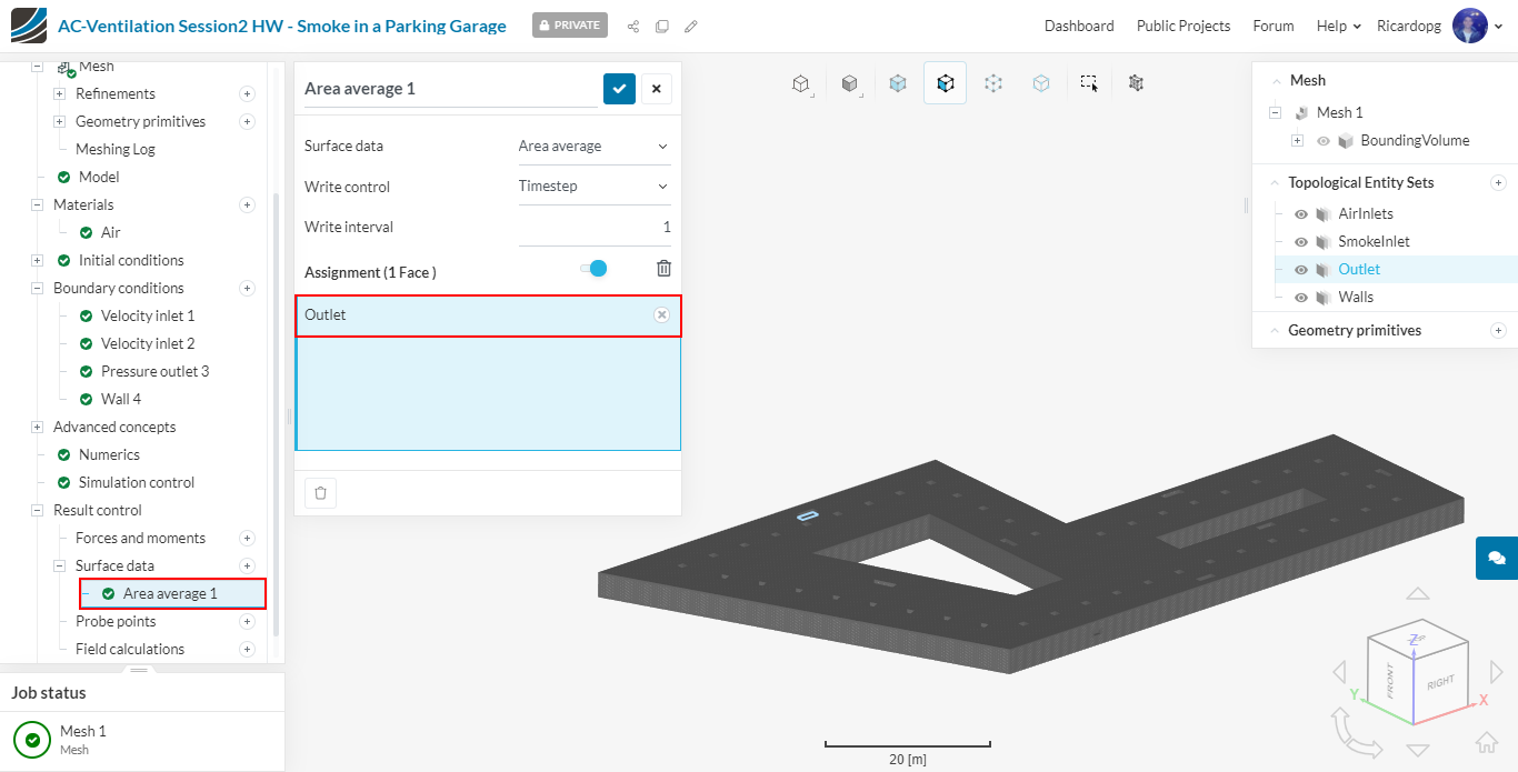
To help us assess convergence, let’s set a Result control . It will be an Area average at the Outlet:
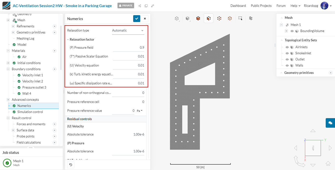
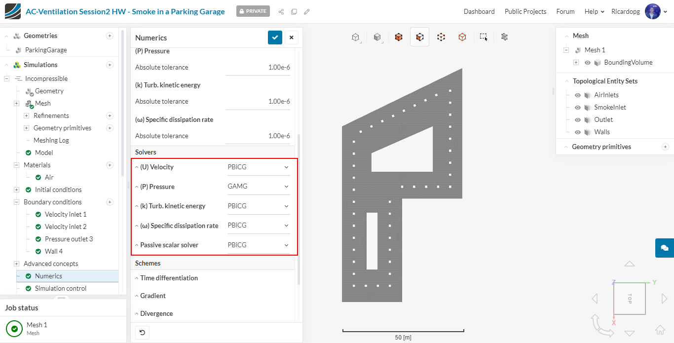
Under Numerics, make sure the Relaxation type is set to Automatic.
Still on Numerics, scroll a bit down to the Solvers section. Switch all solvers except for ( P ) Pressure to PBiCG:
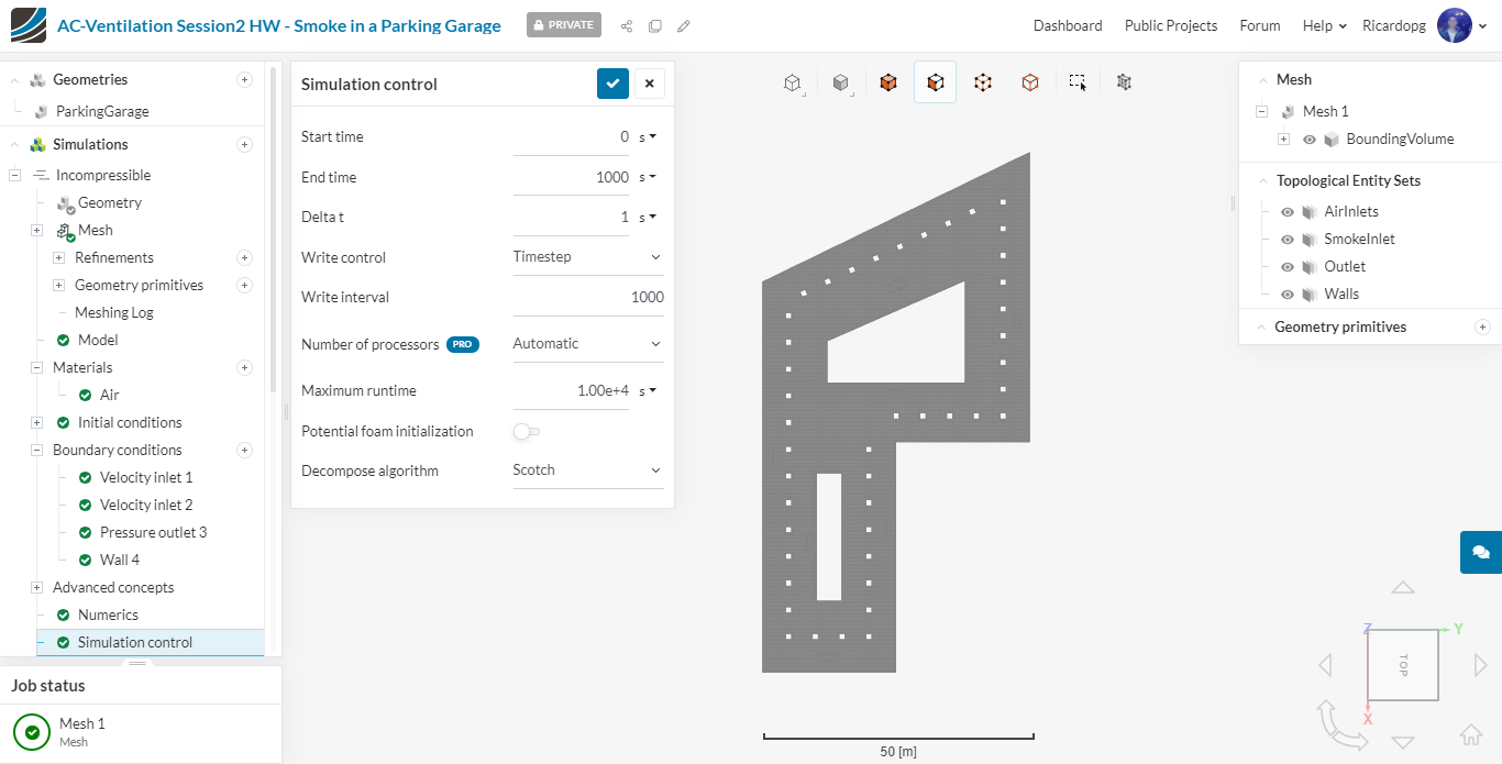
Simulation control remains as default.
You are now ready to run the simulation. Please click on Simulation Runs and Start the simulation.
Post-processing
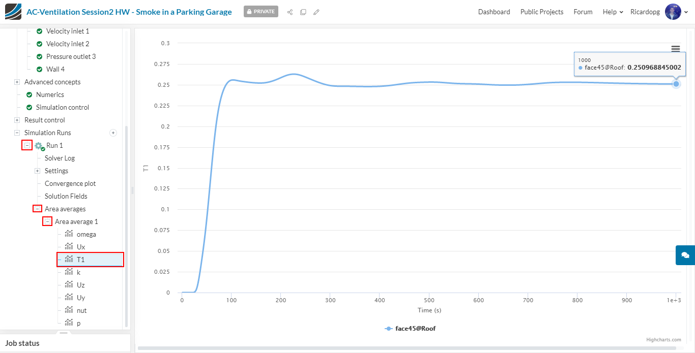
One good way to assess convergence of a passive scalar transport simulation is to monitor T1 levels (passive scalar concentration levels) at the outlet. T1 levels are converging to a value of 0.25.
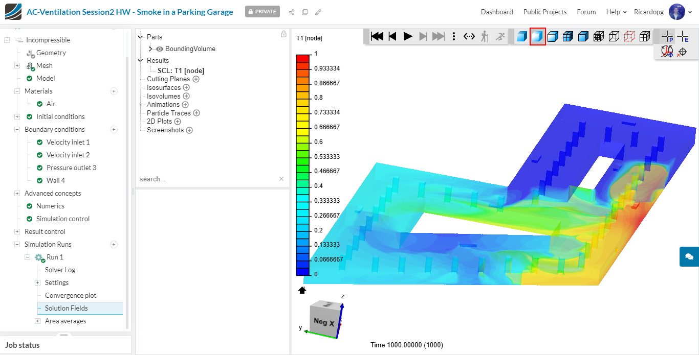
Now let’s head over to the post-processing environment, by clicking on Solution Fields.
Click on Results and select the field you want to plot (T1 for instance).
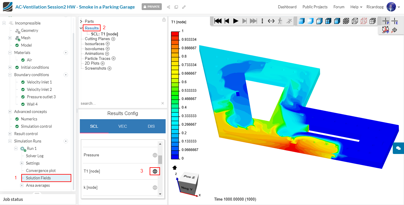
You can make the surfaces slightly transparent by clicking on the Transparent Surface button:
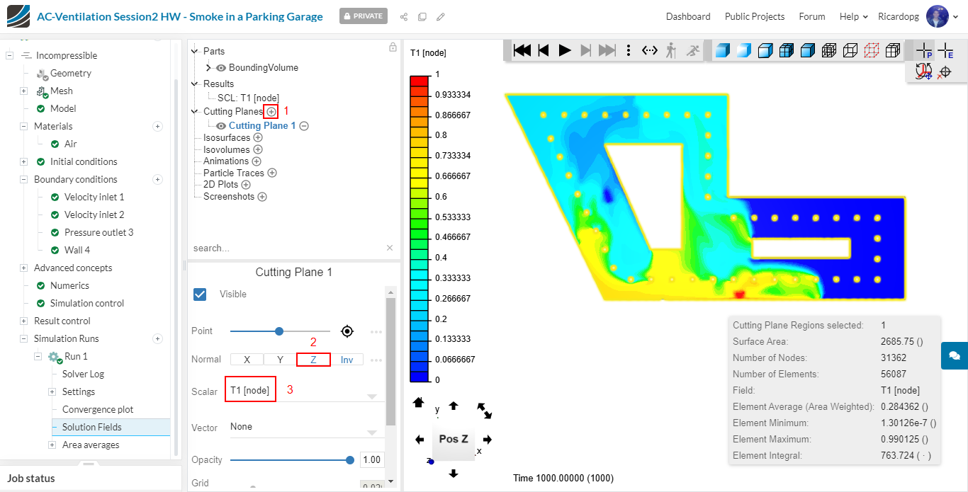
In the post-processing panel, locate Cutting Planes. Click on it to add one. Set the field T1 to plot smoke distribution.
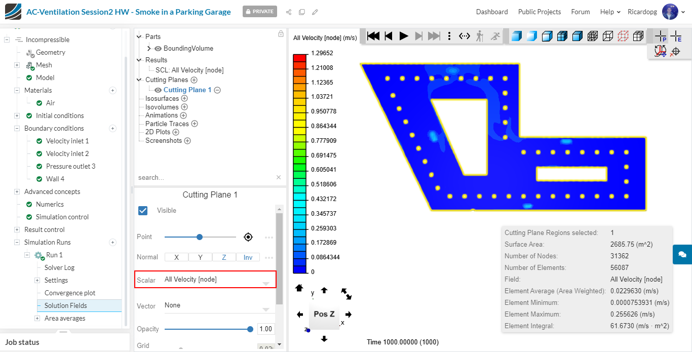
To plot velocity, change T1 for All Velocity:
Adjust the scale to make it more representative:
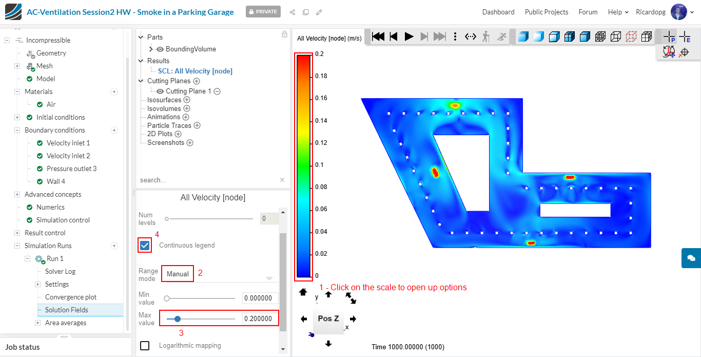
That’s all for the assignment! Feel free to post your questions and results for discussion.