Air Conditioning and Ventilation Webinar
Air Conditioning and Ventilation Workshop (Session 1) ― CFD for Data Center Cooling
Air-conditioning simulation of an office space
Import the project by clicking the link below.
Project Link: SimScale Login
Once the project is imported, the workbench is automatically opened. Then follow the steps below for setting up a convective heat transfer simulation .
Step-by-Step
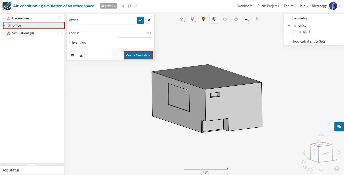
The first step is to create a simulation. Click on the geometry named office and then on Create Simulation.
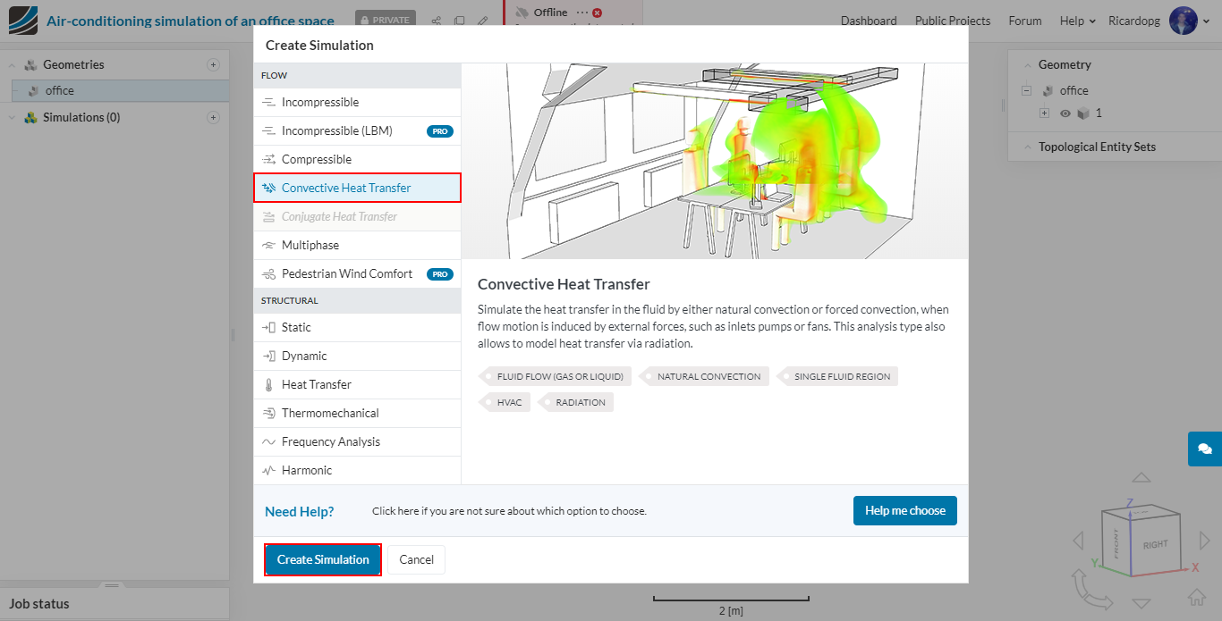
For the analysis type, select Convective heat transfer. Then click on the Create Simulation button.
The simulation tree can be seen in the panel to the left-hand side of your screen. Red entries in the tree have to be filled out in order to run simulations.
In the simulation tree, select the newly created Convective heat transfer simulation and adjust the configuration as shown:
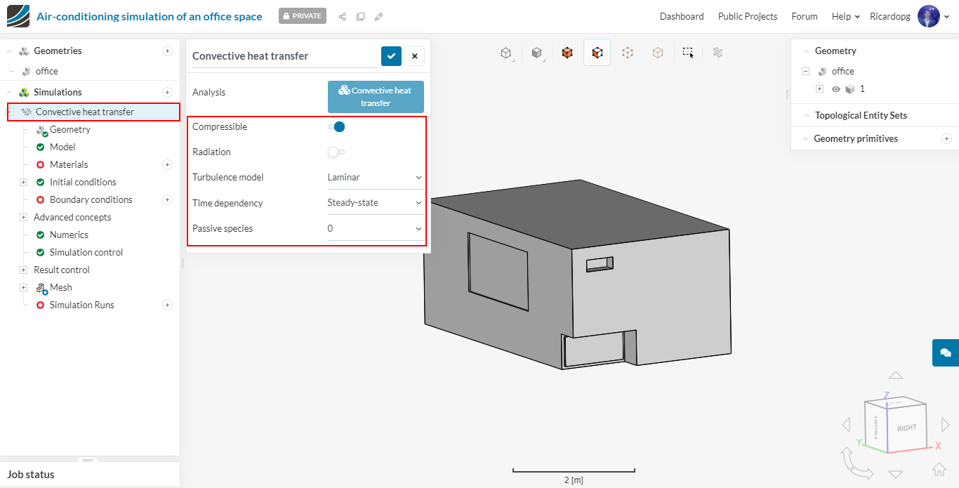
The Boussinesq approximation can be disabled or enabled by the Compressible on/off switch. Note that when Compressible is ON, the Boussinesq approximation is not used.
Meshing
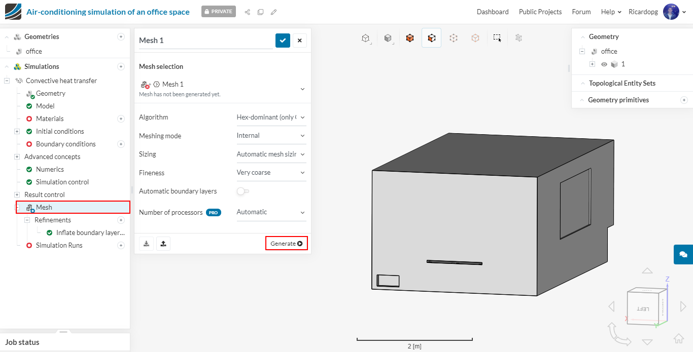
Navigate to Mesh in the simulation tree. Select the Algorithm type to be Hex-dominant (only CFD) and also change Fineness to Moderate. A boundary layer refinement will be set up in the next step, so please disable Automatic boundary layers.

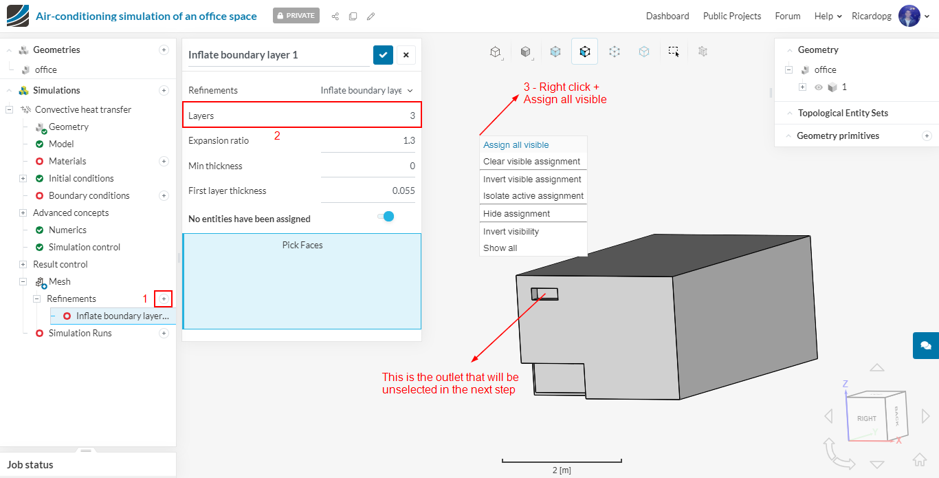
To create a mesh refinement, click on the + icon next to Refinements and select the desired type of refinement.
Layer addition is important to capture the flow phenomenon near the boundaries. Hence layers should be added to all the surfaces except the inlet and outlet. This can be done by selecting all surfaces and then unselecting the inlet and outlet boundaries, as shown in the following 2 images.
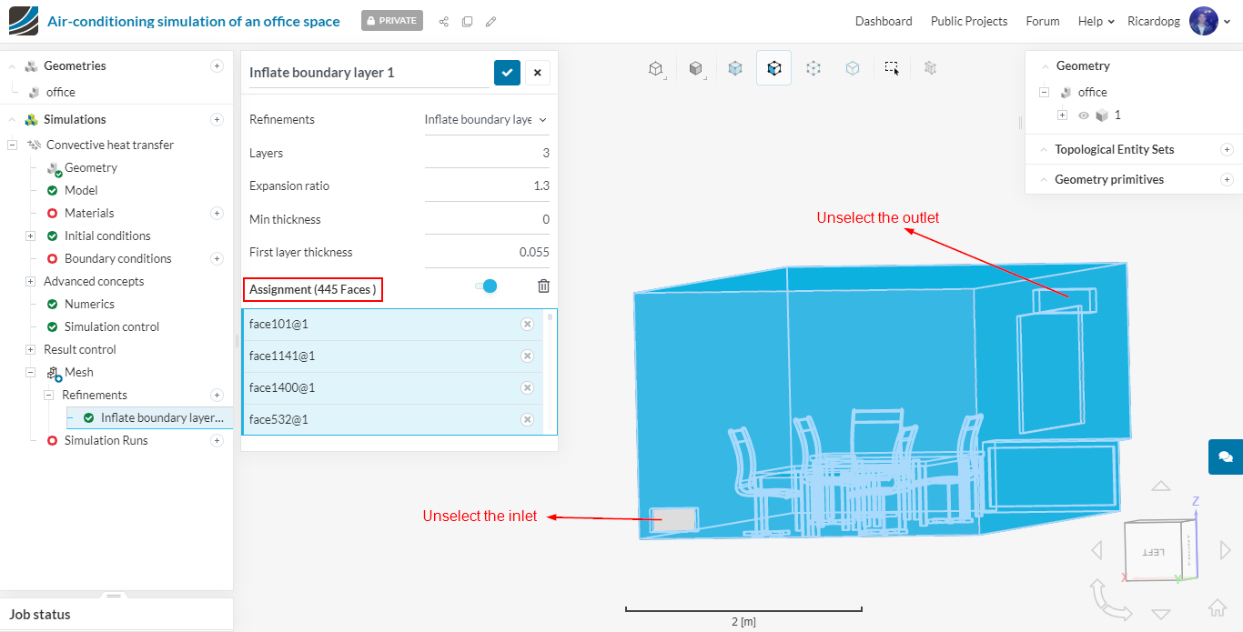
Make sure to check if 445 faces have been assigned. In case of doubt, notice that unselected faces are grey and assigned faces are blue.
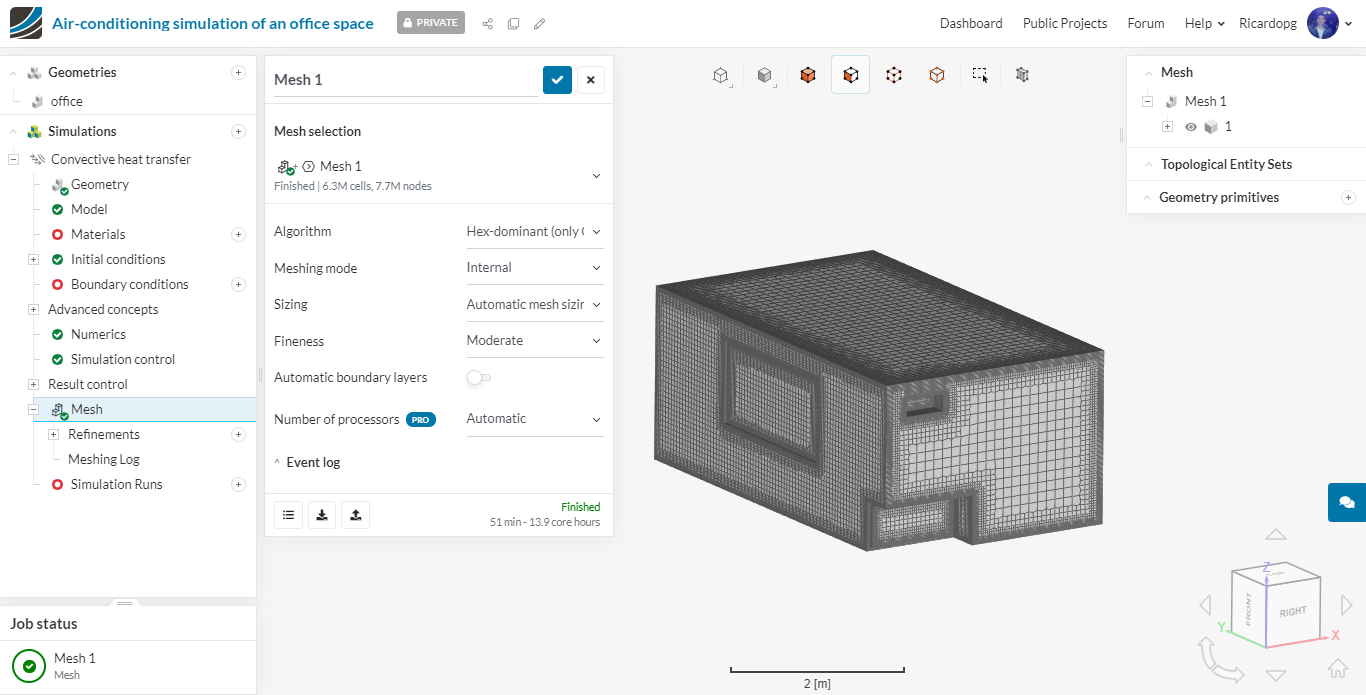
Now, in the simulation tree, head back to Mesh and click on the Generate button. You don’t have to worry with the number of processors that will be employed for this task, as SimScale automatically chooses the most appropriate number depending on the job size.
This mesh operation takes around 50 minutes to finish. It is possible to continue working on the set up while the mesh is being generated.
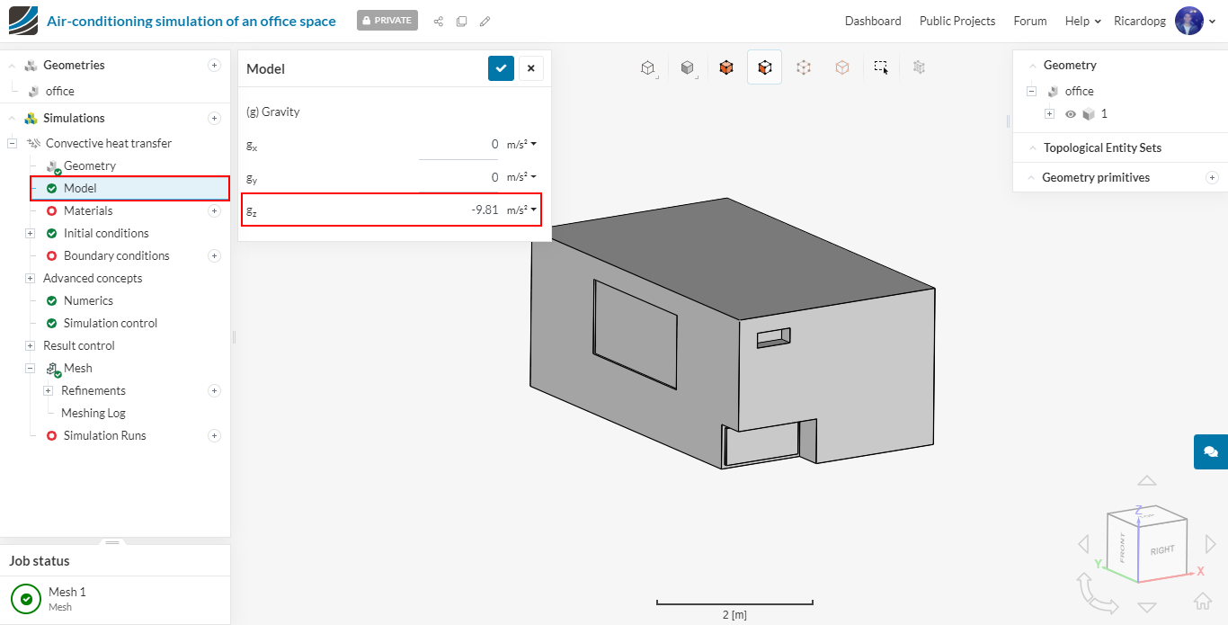
In the simulation tree, click on Model and enter -9.81 in the z direction:
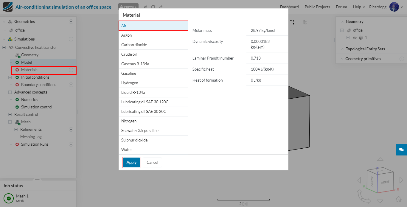
Now please select Materials. Choose Air and hit Apply.
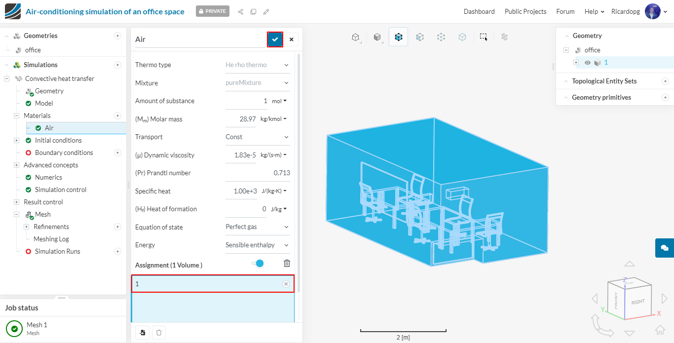
Air is automatically assigned to the flow region 1. Therefore, please click on the blue mark to save.
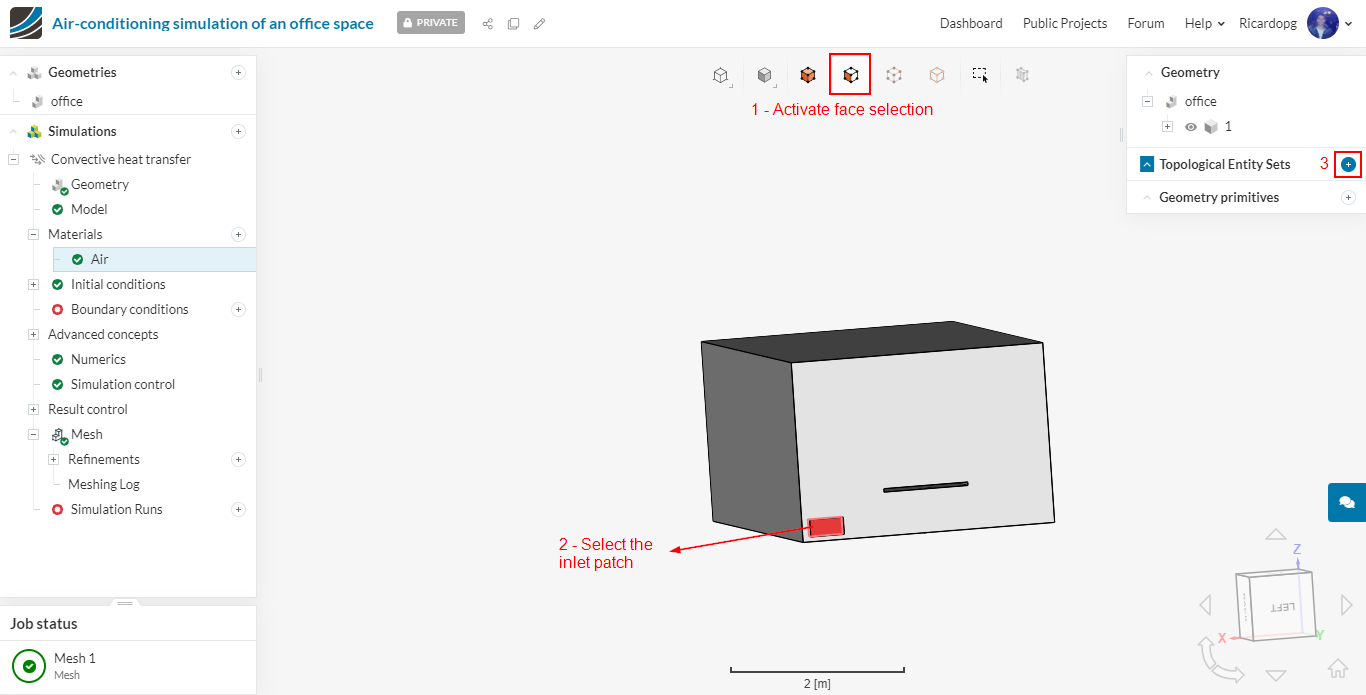
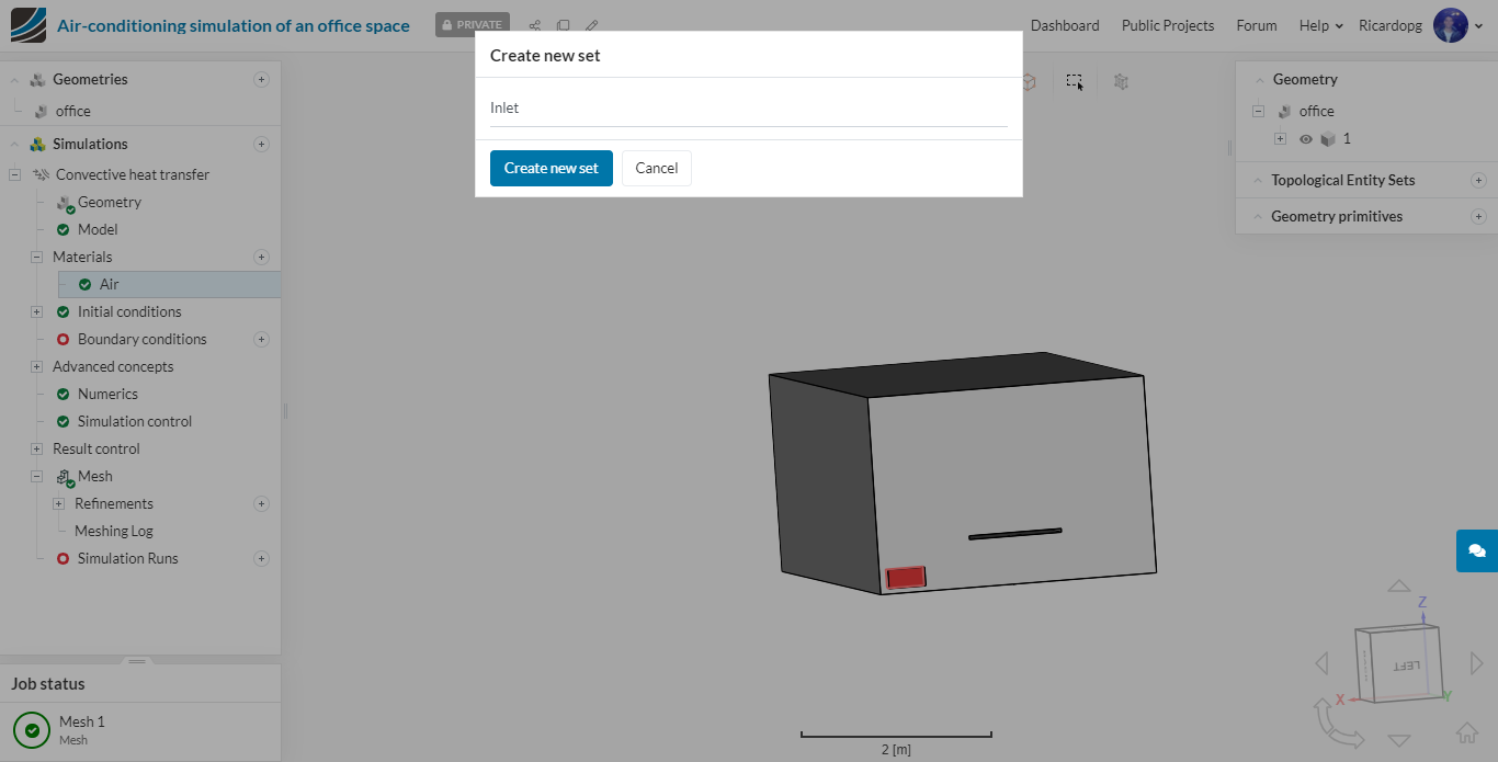
Let’s now create Topological Entity Sets which will help us to set boundary conditions later on. To create a new topological entity set:
- Select the face or faces that will constitute the new set;
- Click on the + icon next to Topological Entity Sets in the right-hand side of your screen;
- Name the topological entity set appropriately.
Creating a topological entity set for the Inlet:
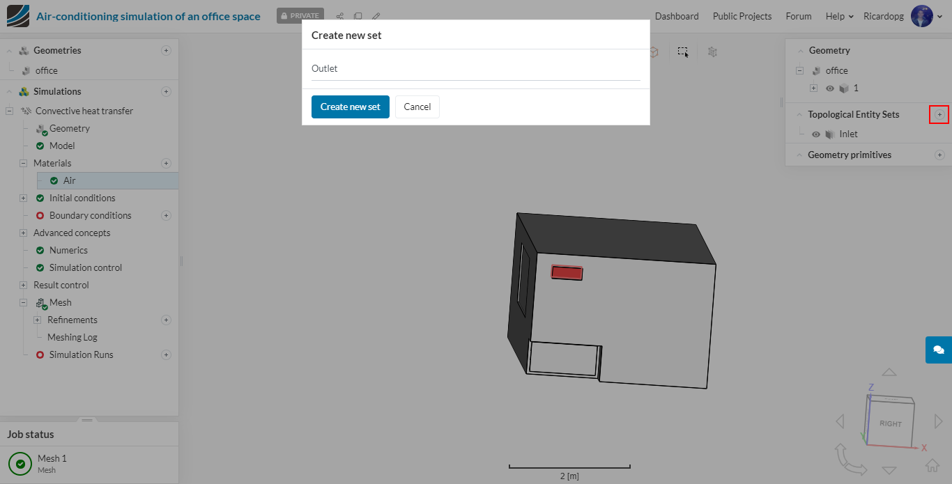
Similarly for the Outlet:
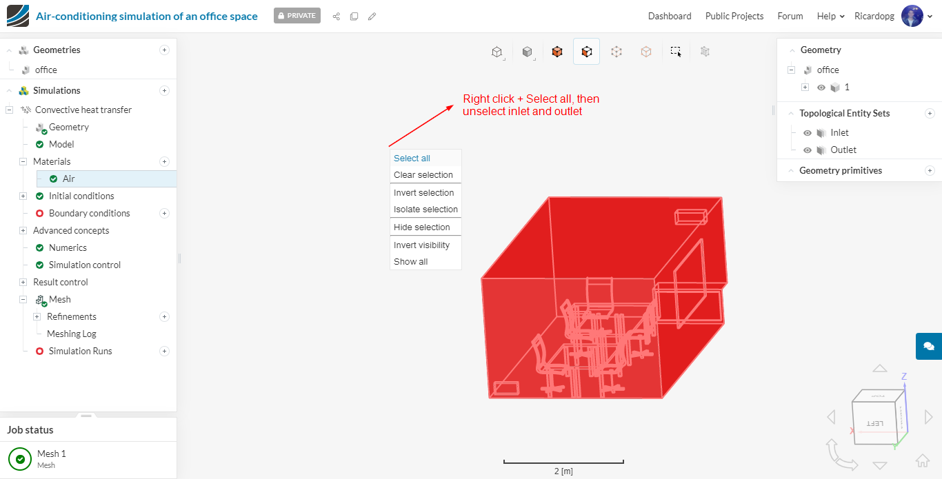
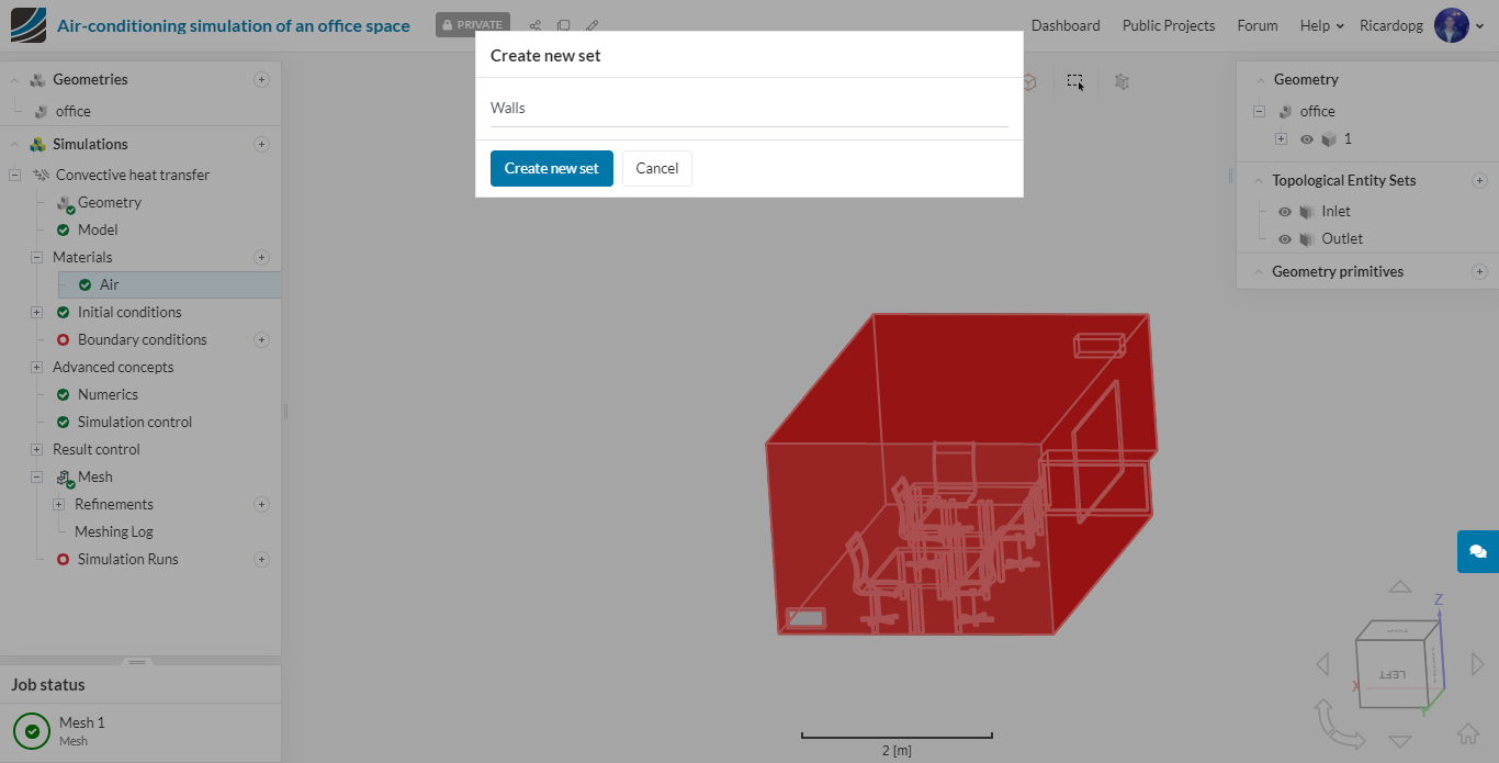
To create a Walls entity set, right click in the viewer and Select all faces, then unselect inlet and outlet:
Under Initial conditions from the tree, select (U) Velocity and enter a Uy value of -0.1 m/s . Then Save these settings

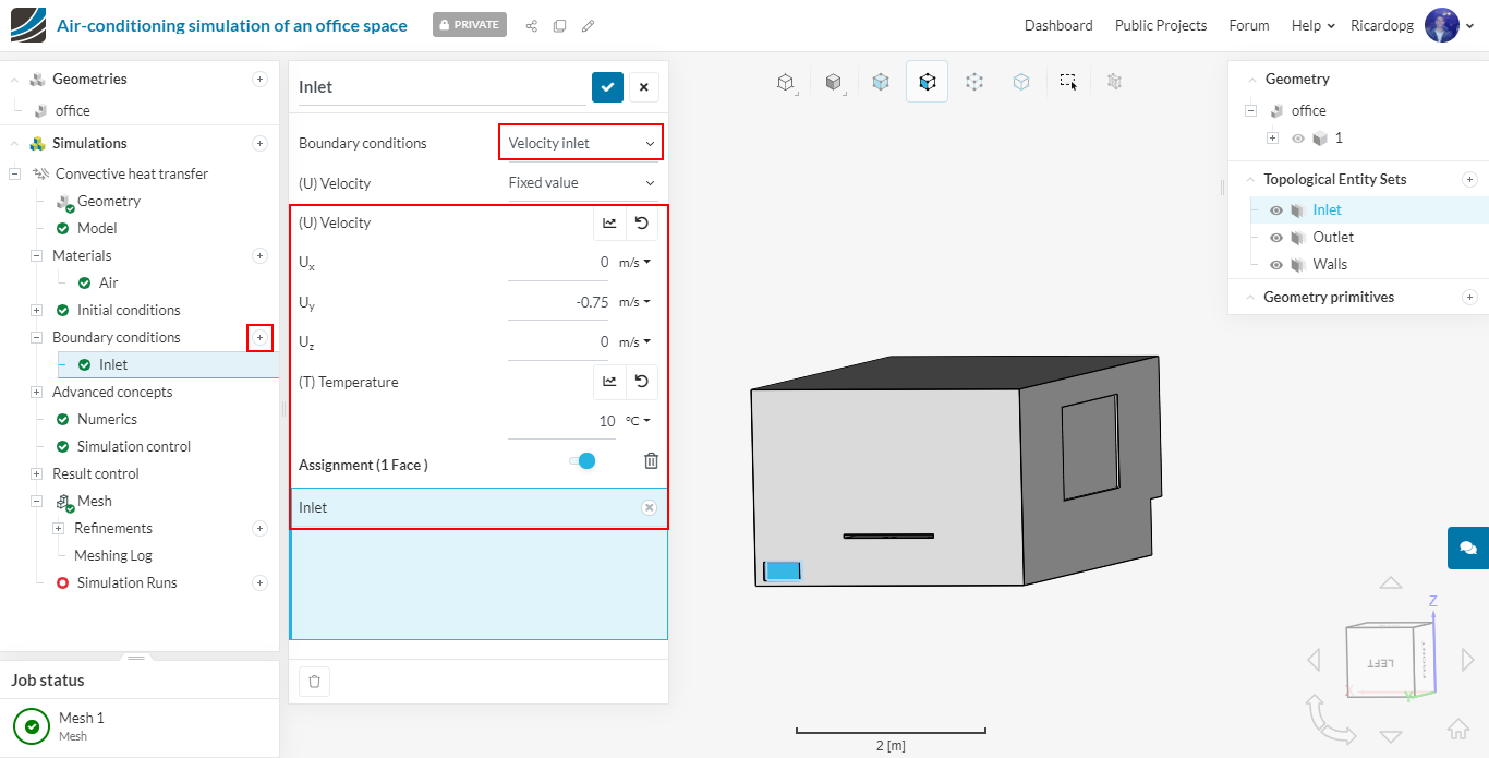
Heading over to Boundary conditions now, we will set up boundary conditions for the previously created topological entity sets. To create a new boundary condition, click on the + icon and select the appropriate type.
The Inlet boundary condition will be a Velocity inlet of -0.75 m/s in the y direction, with 10 Celsius temperature. Assign it to the Inlet entity set:
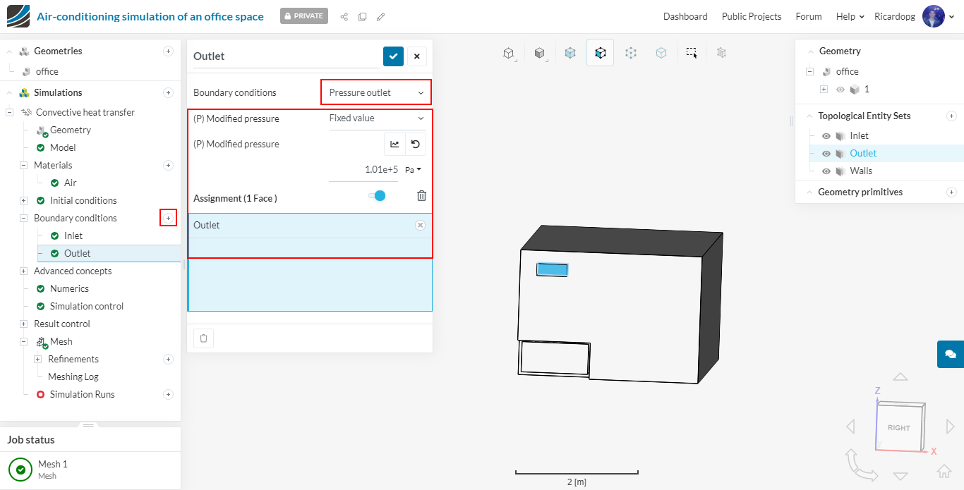
The Outlet is going to be a Pressure outlet condition:
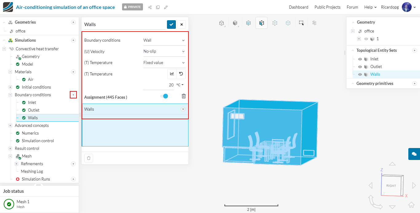
Finally, for the Walls entity set, select a Wall boundary condition with a fixed value of 20 Celsius assigned for the temperature.
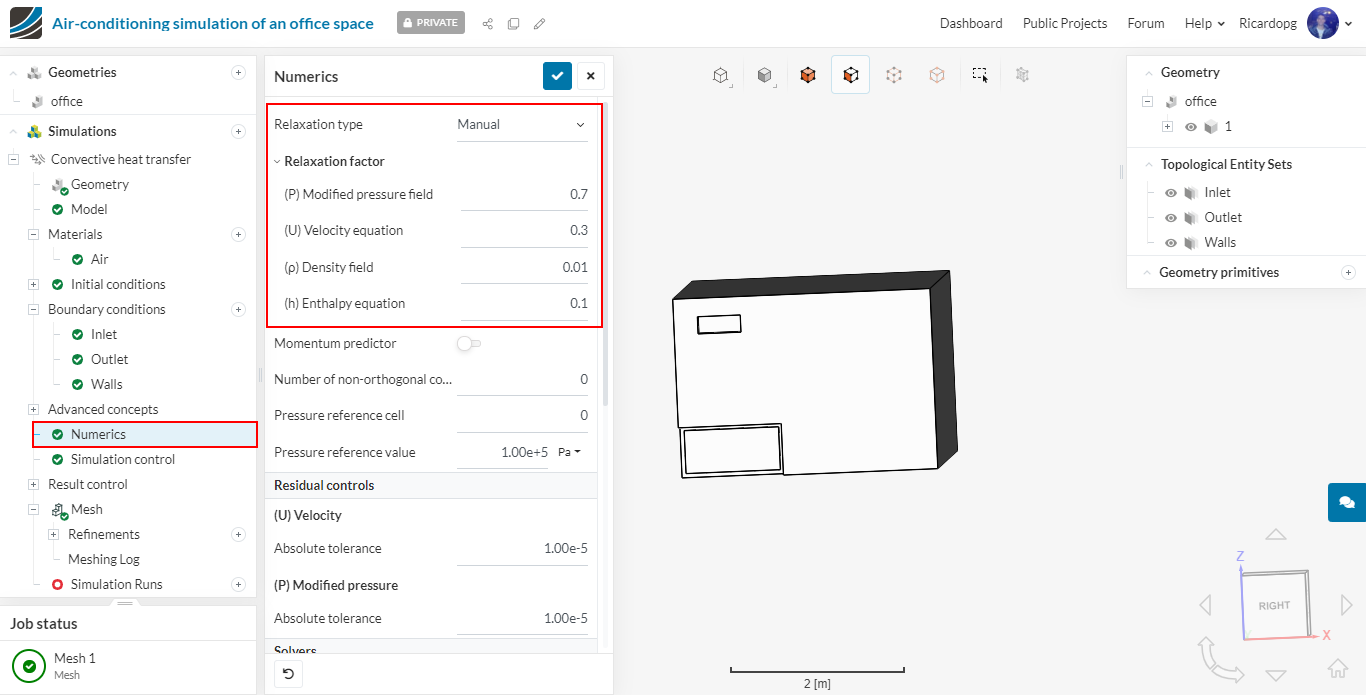
Under Numerics, change the Relaxation type to Manual:
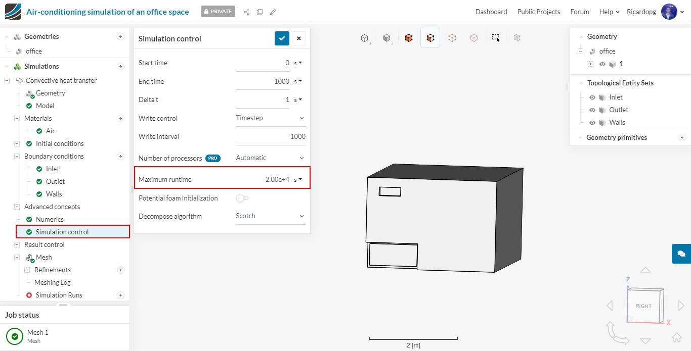
In Simulation control. Please change Maximum runtime to 20000 seconds.
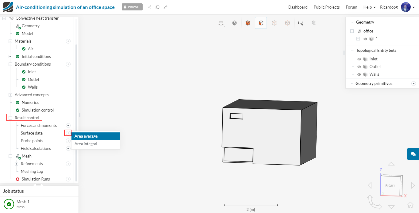
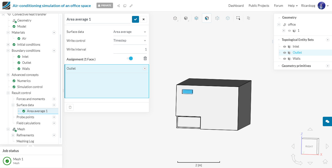
In order to allow us to better assess convergence, let’s set up an Area average Result control on the outlet surface:
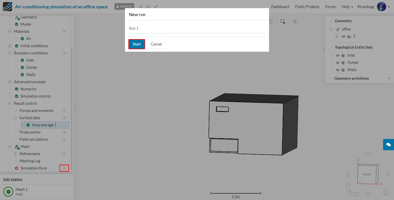
That’s it, now head over to Simulation Runs and hit Start.
Post-processing
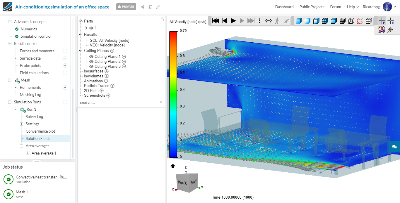
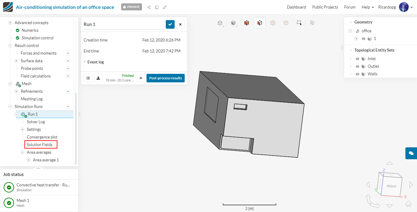
This simulation takes about 75 minutes to finish running. When it’s over, click on Solution Fields to go to the post-processing environment.
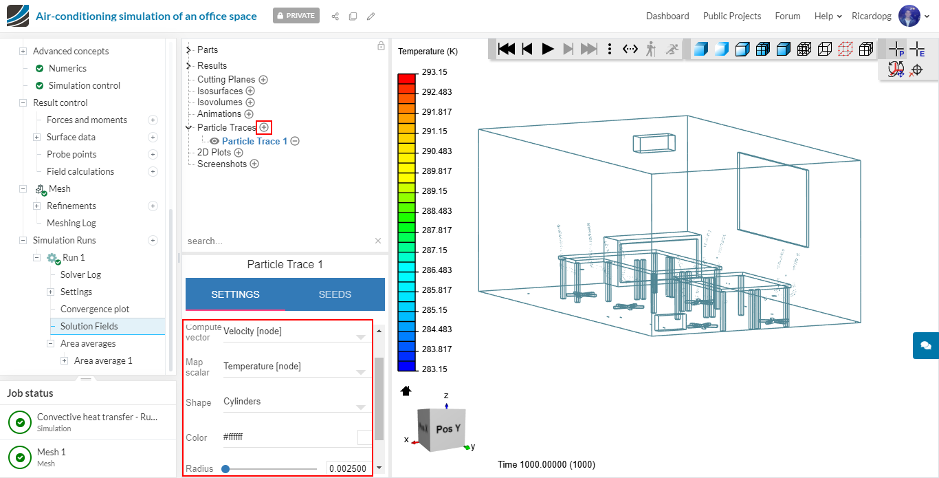
Multiple filters can be found in a panel towards the left-hand side of the screen. Click on Particle Traces to generate streamlines. In SETTINGS, change Compute vector to Velocity [node] and Map scalar to Temperature [node]. Also change the streamlines’ Radius to 0.0025:
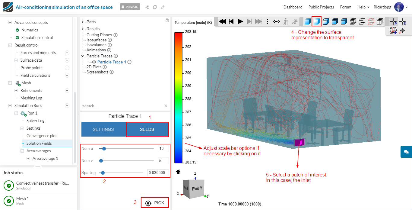
Now, in SEEDS, adjust the number of cells in u and v to 10 and 5, respectively. Spacing between the lines was set to 0.03. The surfaces representation was changed to Transparent surfaces to give it a nice effect. By clicking on PICK and then selecting a face of interest (usually inlet or outlet), the streamlines will be generated.
Now please delete the stream lines by right clicking on Particle Trace 1 and selecting Delete. We will proceed to creating some cutting planes on our geometry.
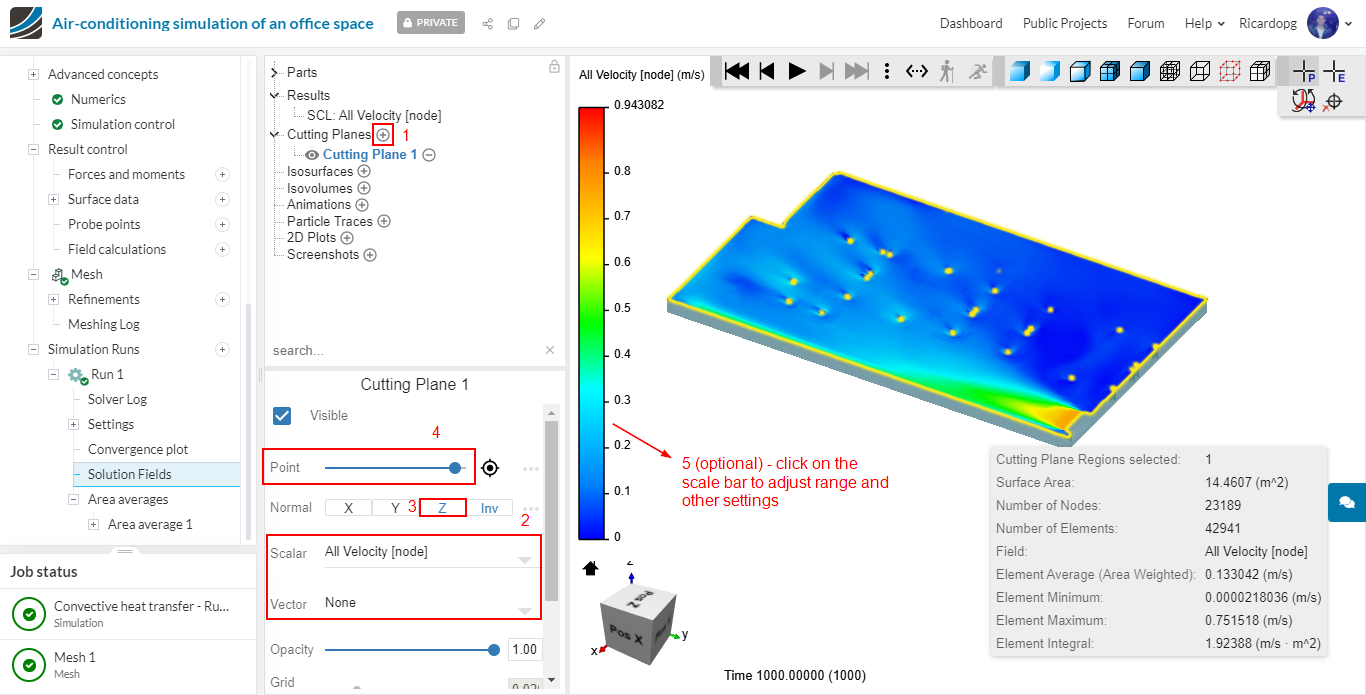
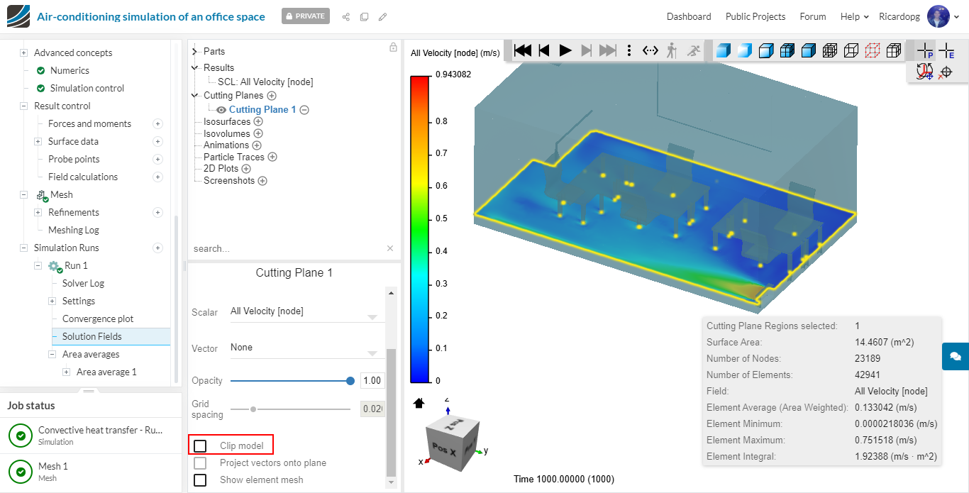
To add a cutting plane, click on the + icon next to Cutting Planes. The first one will be normal to the Z direction. Adjust the sliding bar next to Point to level it with the inlet:
Now scroll down the cutting plane settings and locate Clip model. It is enabled by default. Please disable it. Now the slice is still visible but it’s not clipping our model anymore:
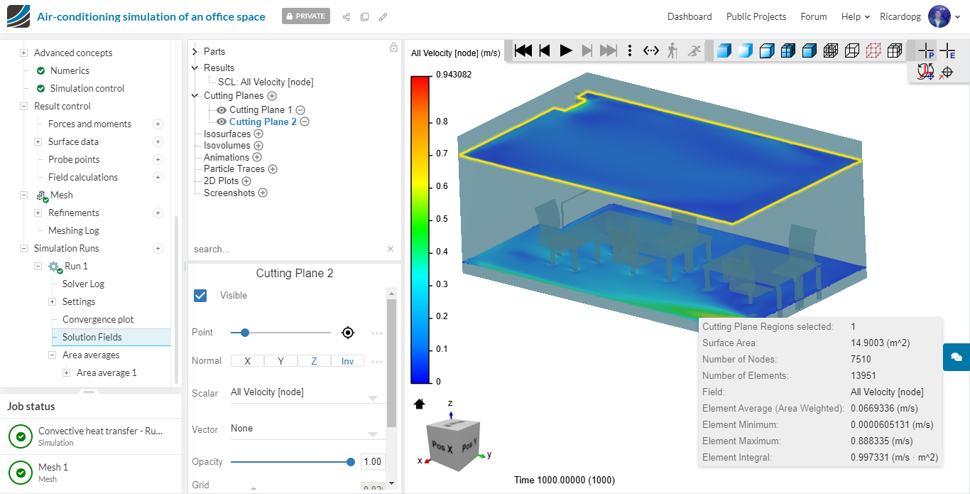
Now add another cutting plane and follow the same steps, but this time place it on the outlet level:
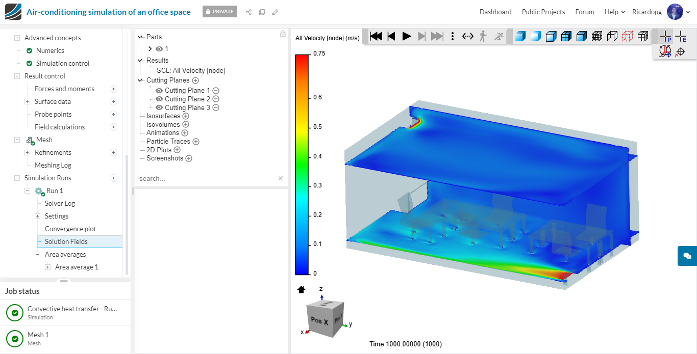
Make yet another cutting plane, this time normal to the X direction and place it so that it shows the outlet:
Now please go back to Cutting Plane 1 and select Velocity [node] to the Vector field. Velocity vectors will be plotted on the slice. Bigger vectors indicate higher velocities.
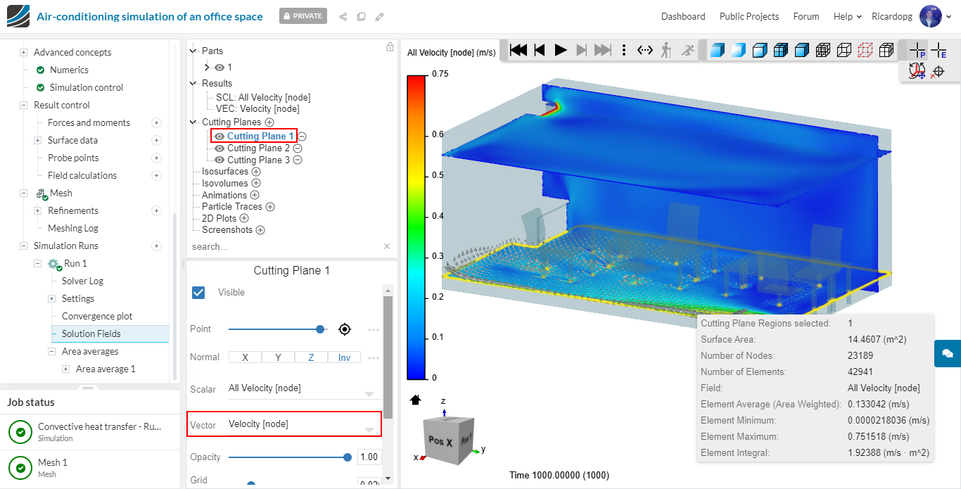
Repeat the process for the other 2 cutting planes: