Reproducing classic flow around a unit sphere

[pegacat]

Hi Folks,

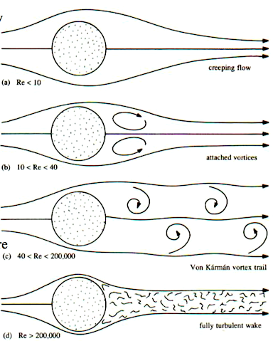
I’m trying to do some simulation work around small (1m-10m) airship drones. In order to calibrate things, I thought I’d try to run a series of flow simulations around a 1m “unit sphere” at different Reynolds numbers, in order to try to replicate the well known experimental results along the lines of:

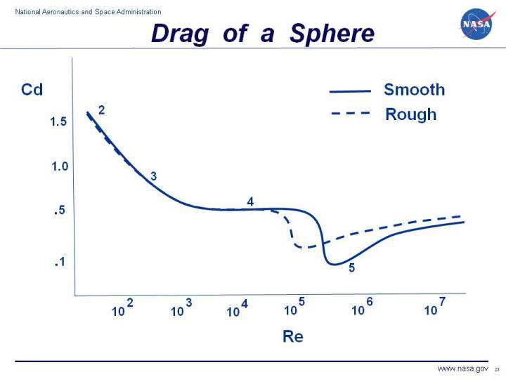
(I’m using Reynolds number as velocity * 1m * 67,567 - is this correct?)

However I’ve had a lot of trouble reproducing these results. In particular I was hoping to be able to reproduce the classic Cd = 0.5 plateau that spans from 103 to 105. To this end I set up a 1m sphere and ran sims with inlet speeds of 0.015 m/s through to 15 m/s, which (I think?) should roughly correspond to Reynolds numbers of 103 through to 106.

Unfortunately my results seem to be nowhere near the experimental results, so I suspect I’m setting up my BC badly!

Reynolds # ~= 1,000
sphere 1m radius: 0.015m/s - drag 0.000264 - Cd ~= 2.5 (k-omega SST)

Reynolds # ~= 10,000
sphere 1m radius: 0.15 m/s - drag 0.00619 - Cd = 0.58 (k-omega SST)
(sphere 1m radius: 0.15 m/s - drag 0.00383 - Cd = 0.36 ?? (LES Spalart - Allmaras) )

Reynolds # ~= 100,000
sphere 1m radius: 1.5 m/s - drag 0.366 - Cd = 0.345 (k-omega SST)

Reynolds # ~= 1,000,000
sphere 1m radius: 15 m/s - drag 32.26 - Cd = ~0.304 (k-omega SST)

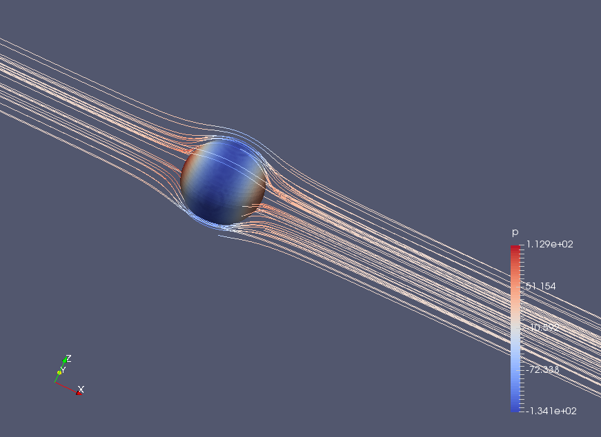
Any ideas on how I should proceed? I think my problem is lack of separation; when I look at the stream lines for all these simulations, they seem to wrap very closely around the back of the sphere; I don’t see any signs of the turbulence or eddies I would expect -

Boundary Conditions for all runs are:
Inlet velocity 0.015 - 15m/s
outlet pressure 0
walls - slip - zero gradient
sphere - no slip - zero gradient
material - ‘air’ from database

analysis type - incompressible - k-omega / transient / PIMPLE (tried LES Spalart - Allmaras once but didn’t seem any better).

Drag calculated in paraview by extracting the sphere as a block, generating normals, calculating normal_x * pressure and integrating…

Any advice gratefully accepted, I’m afraid I’m a complete newbie at this stuff, so most of my values were copied from one of the public car simulations :-)! I suspect I’m not setting things up to model turbulence correctly, as I don’t see any sign of it in the flow calculations, and many of the sphere models show a large ‘-ve’ drag on the rear of the sphere…

cheers,

   - Chris

[dheiny]

@pegacat,

nice simulation project! I’m very interested in the final results! It would be great if you could share them with us! We keep a set of published validation projects also here in the documentation, where this would be a great addition.

But now regarding the project, I guess you’re looking at this This site has moved to a new URL, right?

Without knowing your project in detail, the boundary condition setup makes sense to me.

For the general approach, I’d try to go with the “divide and conquer”: You’re already looking at Reynolds numbers in the turbulent regime, so we’d need to look closer to the values of k and Omega in the initial conditions (what did you choose here?). But also the mesh plays an important role, so this would also need attention. Therefore, how about you start with a laminar flow at low Reynolds numbers, where you can use a laminar solver. There you could validate that the mesh is fine enough (region behind the sphere refined etc.) and you get good agreement there before going into the turbulent flow regime where the turbulent quantities (k, Omega) need to be tuned.

In general, using transient solvers for that problems is I think the right choice.

Any chance that you share the project here via a public link? That way we could have a closer look at the setup.

Best,

David

[pegacat]

Hi David,

thanks so much for the response, and a good idea about trying laminar flow first - however I think for a sphere laminar flow only occurs at very, very low reynolds numbers (<10 according to wikipedia!) For my ‘1m sphere’ I think that corresponds to a velocity of 0.15mm / sec, which is very slow…? I guess if we slowed it down even further we might be able to get to the Stokes drag limit at Re<0.1, but I think for a 1m sphere it would be down to less than 0.00015mm / sec, and I’d start to worry about other types of error?

Anyway here’s a link to my project, and apologies if it’s something obvious, I’m fairly new to all this :-).

https://platform.simscale.com/?publiclink=5414c3c1-7a8d-4b0e-b0c3-1d79ca66e762

In particular, I steered away from messing with the ‘Numerics’ values, and just accepted the defaults - ditto for ‘k’ and ‘omega’. Likewise I’ve used a coarse grained simulation as I wanted to run it repeatedly with different velocities, and I figured that a sphere was simple enough geometry not to need anything too fancy (?). I didn’t use symmetry - I could have stuck it in the corner of two symmetric boundary conditions - basically because I wanted to test things out first and I wasn’t 100% sure how to set the symmetry conditions, and I wanted to minimise the number of things I could get wrong :-).

Thanks again for looking at this! I’m finding it all fascinating, and wondering if I need to blow up one of my meteorology balloons to 1m and take it for a run around the park with a strain gauge :-).

[Ali_Arafat]

Hi @pegacat,

Its interesting to see what you are working on. Well, in my experience its never easy to reproduce an experiment as a lot of things have to be checked before you jump onto the results.

To model flow separation ( or more specifically boundary layer separation ) the first most important thing is to resolve the turbulent boundary layer completely. So you have that setup correctly by using the boundary condition “sphere - no slip - zero gradient” . “zeroGradient” condition for ‘Wall treatment’ will compute the full boundary layer profile that is needed.

Next, It is important that for each Reynolds number your Y+ (y-plus) of the mesh should be between 0 and 1(at max 1.5) for correct physics when using “zeroGradient” .

So, Can you list the Y+ values for the meshes that you used for each Reynolds number ?

…because as the Reynold number increases , boundary layer thickness decreases, you will need different meshes for each Reynolds number so that the Y+ remains in the limit 0 to 1 or 1.5 . Otherwise your results would not be valid.

Another, thing is the size of the domain. It must be large enough so that the flow near sphere is not effected and that the disturbances are almost negligible at the boundaries. Generally the domain is larger for low velocities (Reynold number) and relatively smaller for high velocities.

Further, as David mentioned comes the concern of turbulence values and Mesh Independence studies which play a big role in achieving the right results.

I hope this helps.

Best,
Ali

[pegacat]

Hi Ali,

Thanks so much for the response! I’m reading up on Y+ values now and I now semi-understand them as a general measure of the mesh detail needed close to a wall, however I don’t quite understand how to calculate what they are; online calculators such as CFD Online - Y-Plus Wall Distance Estimation imply you pick a desired Y+ value and from that get the estimated wall distance? In which case my 15m/s case would appear to require a wall distance of 2.3e-5 for a Y+ of 1 at a Reynolds number of 1,000,000.

… which seems an impractically fine mesh?? I re-ran my simscale simulation with a ‘fine’ mesh of 574,000 elements, but at a first approximation it would seem to have a resolution of ~8cm, whereas the figure above seems to be asking for a cell size of 0.023mm??

I think I may have fundamentally misunderstood the limits of CFD - I had assumed that a unit sphere would be a relatively straight forward problem to model, but now it appears it is in fact quite difficult? In fact I don’t require strict physical correspondence, however I do want some confidence when comparing small airship bodies - and at the moment without being able to simulate any eddies at all the numbers I get for Cd seem suspect - the latest fine mesh simulation (another k-omega SST) gave me a drag Cd of 0.15 (half of the 0.3 value I got with a course mesh, which might actually be within range of the physical simulation (if it’s the other side of the dip), except that I see no sign of separation?

Unless I’m misinterpreting things? I attach a screenshot - there still seems to be an unwanted high pressure spot on the back :-/

[pegacat]

Hi Folks,

So with further reading, the answer seems to be that this isn’t really practical; between the range of velocities I’m looking at (~.1m/s to 15m/s) we have a number of different fluid flows regimes, each of which has different properties and requires a different mesh and analytic scheme - so in a sense I need to know the answer before I can model it, and would required a separate setup for each Re range as per the figure below.

(Figure from S. Vogel, Life in Moving Fluids, Princeton University Press, 1994)

… so I guess at this stage I’d be satisfied with just being able to model the fully turbulent, high reynolds number condition which is of most interest to me. If anyone has any hints as to how I can set up simscale to do this I’d be grateful; I’ve made a number of attempts at what I believe is a Reynolds number = 1,000,000 simulation for a 1m sphere traveling at 15m/s - this is around 30 knots, a speed at which I know there should be a significant turbulent wake - but as you can see from the image above (unless I’m massively misinterpreting things) the simulation is still showing what appears to me to be very low Re ‘creeping flow’.

For example, are the default values for k and omega satisfactory here, or should I tweak them?

cheers,

[Ali_Arafat]

Hi @pegacat,

I was wondering whether you managed to get the results you were looking for or not.

To help you out, here is some additional theory of what to expect for Re = 1e6. This was taken from free online MIT course lecture.
I will highlight some important things from page 73-74 below:

The first is as you already mentioned regarding the flow regime at Re=1e6. The thing to point out here is that you have a “Turbulent boundary layer” both upstream and uptill the separation point.

To model “boundary layer separation” accurately it is important NOT to use “wall functions” but to resolve the flow completely by setting the option to “set gradient to zero” in the wall boundary condition. For this Y+ of less than 1-1.5 must be ensured.

In this case separation takes place farther around toward the rear of the sphere, at a position about 120–130° from the front stagnation point. The wake becomes contracted compared to its size when the separation is laminar, and consequently the low pressure exerted on the surface of the sphere within the separation region acts over a smaller area. Also, the pressure itself in this region is not as low (Figure below).

Figure by MIT open course ware
.

So, try to do the following:

1- See if you get a similar normalised pressure profile on the cylinder as shown in figure above (the lower graph)
2- and check if you have flow separation behind the sphere by plotting the “wall shear stress” on the sphere.

Then you will be able to better decide which type of flow you are getting ( i.e low or high Re)
Also for Re = 1e6 you will get a lesser drag value than Re < 1e6. This is called “drag crisis”. Also mentioned in the document page 74.

As for the calculation of K and Omega in ‘Initial conditions’ use the values based on formulation given here " K-Omega formulation" . ( use second formula for Omega)

I Hope this helps.
Best,
Ali

[pegacat]

Thanks for this Ali!

Alas, I’m out of time for this exercise at the moment - the sphere exercise was to attempt calibration for both an ellipsoid and an annular airfoil; but I think even if I am successful with the sphere, it wouldn’t guarantee an accurate simulation for the airfoil, so I’ll need to return to physical testing.

Thank you so much for your help, and I’ve grabbed your references in the hope that I’ll get a chance to return to CFD in the new year.

cheers,

   - Chris

[dheiny]

@pegacat,

would it be possible that you make the unit sphere project public? That way other community members could finish the validation project. Would be a great addition to the set of validation projects.

Regarding physical testing: Generally I don’t think of simulation always as a method that can be used instead of physical testing for product development. Using them in combination can be very powerful. Having a simulation setup that was validated by physical testing allows you to run many more design variants than using physical testing alone. But I can understand that depending on the project time might be tight. You could think of creating also a public project for it to get some support from the community on it.

Just some ideas

Best,

David

[pegacat]

Hi David,

I’m not sure how to make it a proper public project, but I generated a public link to the project above? (or more recently: https://www.simscale.com/workbench?publiclink=b2b6ebf7-2851-4e6c-9f22-465651c0ba71)

…under ‘share’ I only see the option ‘generate public link’ or ‘invite to project’ - is this what you mean, or is there some other way to make it public? (I’m perfectly happy to do so, but since I don’t think I’ve got my initial conditions correct, it’s more likely to mislead people than help them!)

Anyway, thanks again to everyone for the pointers; I just wish I had the time to give this the attention it deserves!

cheers,

Chris

[dheiny]

Chris @pegacat, - to make it a public project, click on “Actions” on the project overview page, then “Edit project properties” (see screentshot below)

At the bottom of the project overview page, you’ll see the slider button “Visibility”. If you put that one to “Public” and hit the “Update project” page, everyone can see the project an create copies from it.

I think you’re almost there with this project, so I’ll see if we can get some community members involved to finish this project. @Ali_Arafat, @gholami - what do you think?

On a related note: Without a validation via physical testing, there’s probably never such a thing as “guaranteed accurate results”, but there are different methods to test your simulation results such as mesh independence tests, changing the order of your numerical schemes, checking on the behavior of integral physical quantities etc. . There are no resources yet in the documentation on this, but we probably should add a description of these methods to help in such situations.

Thanks for sharing your project!

Best,

David

[pegacat]

Hi David,

thank you! I’ve set it to public, please feel free to look around!

I’m not really looking for physically accurate results, just something ‘good enough’ to do comparative drag calculations with between different small airship shapes :-).

cheers,

Chris

[dheiny]

@pegacat - great, thanks for sharing! Let’s see if we can get this finished

[dheiny]

@pegacat - good news, @Ali_Arafat will soon start working on finishing your unit sphere project. We’ll keep you updated!

[pegacat]

That sounds grand - I’ll be very interested to see how someone with the right skills manages it :-).

I think it would also be a useful baseline for a certain class of flow problems as well…