Many conjugate heat transfer simulations include geometries that have very thin, detailed air gaps. These types of small channels can dramatically increase cell count in the domain, and can cause divergence issues due to poor mesh quality in the fluid domain. At times, time and effort can be saved by approximating the thin fluid gaps by a solid region with material properties of air. By doing this, convection is ignored and the only mode of heat transfer considered is conduction. Generally this is valid in thin sections, but as a region/gap gets larger, the convection effects become more dominant and this approach is no longer valid.
The Rayleigh number is a dimensionless number used to describe the relationship between buoyant and viscous forces in the domain. A Rayleigh # of ~1700 is a critical value at which values higher represent convection-dominant flow and values lower represent conduction-dominant flow. Below is the equation for Rayleigh number:
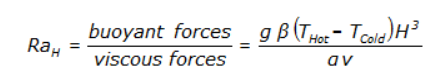
Where:
g = Gravity
Beta: thermal expansion coefficient (~1/323.15 for air)
a = thermal diffusivity of air
v = kinematic viscosity of air
T_h = localized hot temperature
T_c = localized cold temperature
I decided to generate test case to evaluate the Rayleigh # and validity of the ~1700 threshold. I ended up creating this natural convection electronics cooling project.
The geometry originated from a Raspberry Pi GrabCAD project.
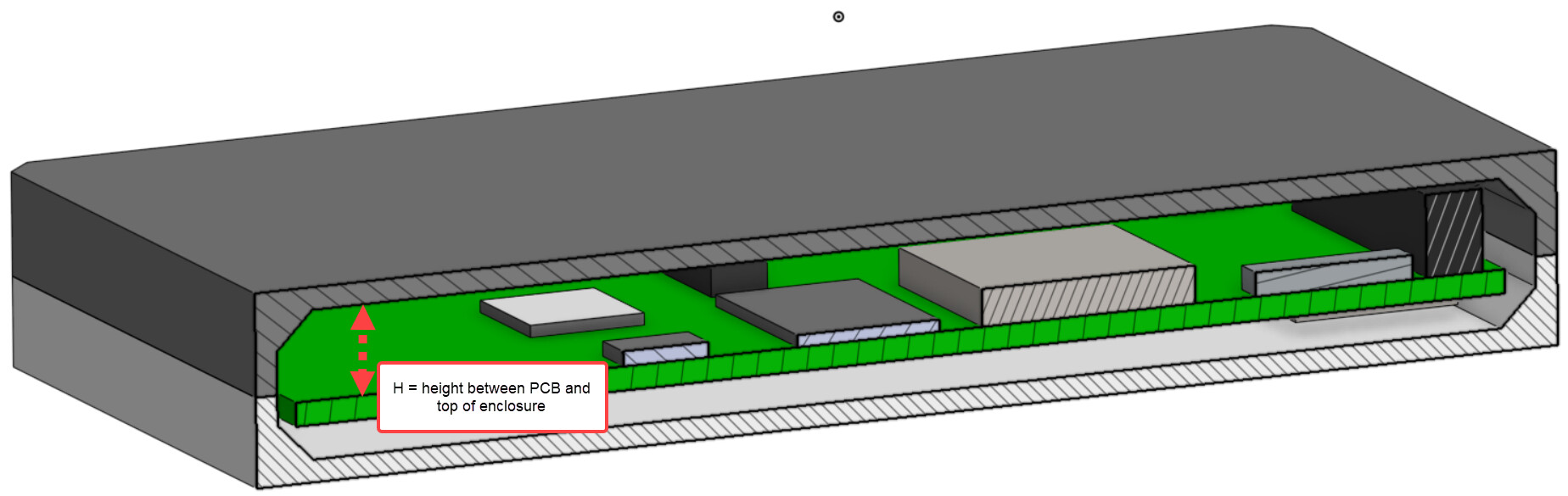
I parameterized the distance between the PCB and top of the electronics enclosure and considered heights of 6, 10, 14, and 18 mm.
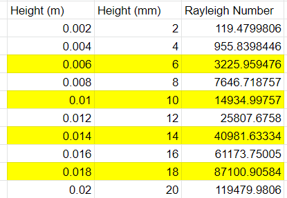
In the table above I show the calculated Rayleigh numbers. Rows in yellow highlight the distances I ran simulations at. Although the critical value of 1700 represent a gap height of 4.85 mm, I decided to try larger gaps as gaps less than that did not make a lot of sense in terms of enclosure design/packaging. For each distance listed I ran 2 simulations: 1 simulation only considered “solid air”/conduction in the enclosure and 1 simulation explicitly modeling the air as an ideal gas. Next, I plotted the difference in max chip temperature at each of the gaps:
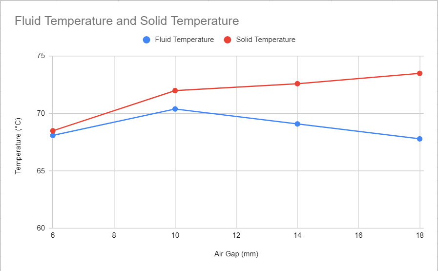
Interestingly enough, a gap of 6 mm (Ra = 3200) still showed good correlation between the 2 sets of results, with only about 0.5 degrees C in difference. 10 mm gap still showed good correlation with the solid air only over predicting temperature by about 1.5 degrees C. After 10 mm (Ra = 14,900) the correlation between solid air vs. ideal gas increased dramatically and it became invalid to use the solid air modeling approach.
A few final comments:
- Evaluating Ra requires knowing the localized high and low temperature at your gap; without test data this is not possible to get without running an initial simulation. Perhaps using Solid Air could save time with additional simulations beyond the first, or perhaps the user has an idea/intuition about appropriate values ahead of time.
- SimScale does not currently support temperature dependent thermal conductivity values; I chose to use a k value of air at 30 C, but temp dependent material properties could further improve correlation.
- “Solid Air” may be a best approach for initial “quick and dirty” simulations in which you want to avoid divergence or time consuming geometry defeaturing. Ultimately it may make sense to do a final run with fluid air.
- Using “solid air” will reduce run time because BL cells will not be included in the “solid air” and only 1 equation, conduction, will be solved for in those cellls.
Relevant links: