Hi! Just got a short question on your usual workflow.
Generally i simulate my cfd cases for 1000s. After that i export the csv data of the coefficients. I just average the steps 900-1000s to get my final drag/lift coefficients in numbers. How do you guys interpret the graphs?
Hello @mwipprecht , that’s a very good question in my opinion indeed. I assume you are talking about averaging the oscillating flow coefficients when the simulation type is set to steady-state, is that correct?
In this case, it’s best to ask the question whether the problem has a steady-state solution, or not first. By nature all problems will be transient, but some of them will have almost steady-state solutions as well. In case the problem is highly transient (seperation behind the wing, buffeting, etc.), flow coefficients may still oscillate while using steady-state approach even though I generate very fine mesh structure and use very accurate models.
If I’m confident that the problem should have a steady-state solution and my flow coefficients are still oscillating, I would check my mesh and simulation settings.
In either case, I followed the same workflow as you desribed though while generating aerodynamic databases for aircrafts. I had high seperation zones when the angle of attacks or side slip angles are relatively higher so I needed to average the flow coefficients using last 100 to 500 iterations. Then I was able to obtain nice and smooth lift/drag curves.
I’m curious about other users approach on this too so let’s see if there are further inputs here.
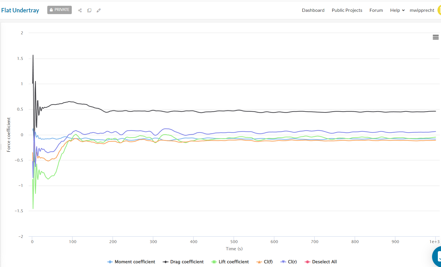
@kaany Yes, you understood my case. Its a steady-state sim, but for e.g. drag coefficient close to 600s is about ~0,43 and in the end its ~0,46
I averaged the last 100s, so my result is 0,448
also the lift coefficient is interesting. sometimes + somtimes negative, so i also averaged the last 100 steps. But is this really the best result ? I´m a little bit unsure about that.
Hello @mwipprecht ! Glad to see you have this case running effectively, I believe I helped you a bit with meshing last year (unless you picked this geometry up from that user).
Anyways…I just wanted to chime in a bit as I have some extensive industry experience in motorsport CFD. The approach you are taking to average the steady results over iterations is common in practice, and it is reasonable assuming your variation (std. deviation) is not too large compared to your expected accuracy. In fact, even in wind tunnels averaging of the forces and moments must be done to arrive at a single coefficient, as there is always some inherent instability in the flowfield and force/suspension apparatus.
For a RANS simulation on a vehicle like yours, CD variation of 0.5% is reasonable, so striking the average over one period cycle near convergence is fine. It is not uncommon for CL to take longer to converge and to have more eventual noise, mainly due to underbody fluctuations near the tires, rear diffuser, and front splitter/undertray (if applicable). When the overall CL is near zero (as in your case), this can be even more true as there isn’t a large amount of underbody pressure or suction to “force” a strong/steady solution.
I would suggest dumping snapshots of the upper and under body CP/pressure at various intervals along your simulation (say every 100-200 iter.) to see the sources of the noise. In these areas, improving the mesh quality via CAD cleanup or mesh refinements would help tighten up the CL value. After all, residuals are nothing more than remaining numerical error which manifests itself as unsteady behavior in a RANS simulation. This error is much harder to tease out in an unsteady simulation!
Keep us posted on your progress, so that others in the SimScale community can learn from your work!