The fixed coefficients porous media model is sometimes used, especially for compressible flows, to predict the amount of pressure drop that will take place due to the incoming flow.
The main objective of this article is to discuss the workflow to derive the alpha and beta coefficients based on experimental data. In our scenario, the “real life” geometry consists of a pipe with a perforated plate, partially blocking the flow.
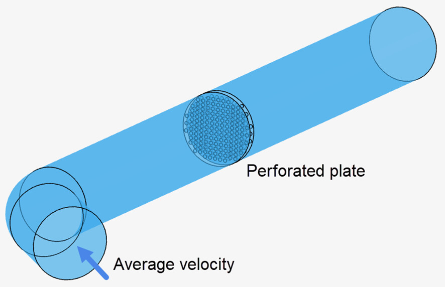
The fluid moves through the pipe at an average velocity, causing an additional pressure loss to occur as the fluid goes through the plate.
The following test data for Average velocity versus pressure drop through the perforated plate is available:
| Average Velocity (m/s) | Pressure Drop ( Pa ) |
|---|---|
| 0.5 | 1176 |
| 0.7 | 4620 |
| 1.0 | 10410 |
| 1.2 | 18460 |
| 1.5 | 28700 |
| 2 | 40920 |
Like many of the other porous media models (Darcy-Forchheimer, Pressure loss curve, etc.), the Fixed coefficients model is based on a polynomial approximation of the form Delta P = x.U + y.U^2.
More precisely, the formula below is used:
\Delta P = \alpha.p_{ref}.t.U + \beta.p_{ref}.t.U^2
Where:
- \Delta P (in Pascal) is the pressure loss experienced due to the porous media,
- ρ_{ref} is the density of the material (in case of incompressible flow) or the Reference pressure (in case of compressible flow), in kg/m3. The reference pressure is defined within the fixed coefficients window
- t is the thickness of the porous media in the flow direction (meters)
- α and β are the model coefficients, which are input in SimScale
Therefore, now we need to do a polynomial curve fitting of second order to obtain a correlation that looks like the formula above. This can be done in various ways, e.g. in MS Excel:
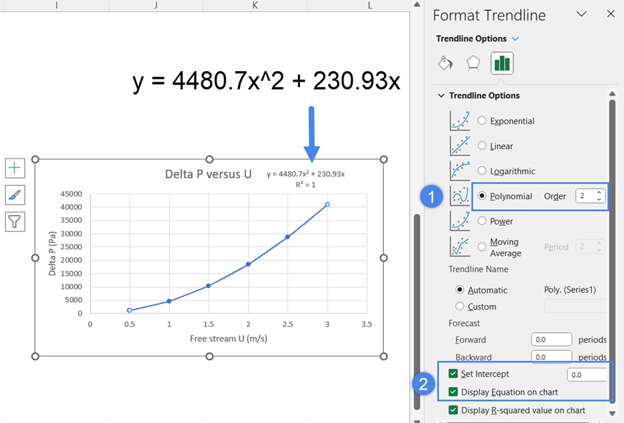
Once the correlation is extracted from the graph, it’s just a matter of comparing the two equations and obtaining the alpha and beta coefficients.
In this case, the perforated plate is 0.01 meters thick, and the density is 1000 kg/m3. Therefore:
β=4480.7/(ρ_{ref}.t)=4480.7/(1000*0.01)=448.07
α=230.93/(ρ_{ref}.t)=230.93/(1000*0.01)=23.093
These are the coefficients in the flow direction. In case of an isotropic porous medium, the same coefficients can be used in the other directions as well. If the flow perpendicular to the flow direction is blocked, then you can multiply the alpha and beta coefficients by 10-100 in the blocked directions.
This way, the user can run a simulation with a simplified porous media to account for the pressure drop through the complicated CAD geometry. As a reminder, the best practice is to have at least 5 cells across the thickness of the porous media in the flow direction.