Greetings to this awesome Forum!
As I have seen multiple questions about the topic of mesh independence and convergence of results against mesh refinement in FEA simulations, I would like to properly tackle it with a practical approach. Thus I will mix some basic concepts and an application example you can follow along, as a reference for your future cases.
1. Basic Concepts
In the Finite Elements Method (and other Galerkin’s method based numerical techniques), we approximate the solution fields (displacements, stresses, strains, temperature, etc) from a continuum volume using a mesh, which is composed of a finite number of points (called nodes)and the elements connecting them. The fields are computed at the nodes, based on differential equations that describe the physical behavior.
As a general rule, the quality of our approximation depends on the adequacy of the mesh to properly capture the variations in the fields of interest. Put simply, adequacy means that there is a sufficient amount of mesh nodes and that they are located in the right places, such that our approximation is similar enough to the physical field.
Mesh refinement is no more than the process of adding more nodes and elements to a mesh, and to locate them strategically in such places where they will improve our numerical approximation to the physical fields.
Having this in mind, let’s jump into a practical example.
2. Practical Example
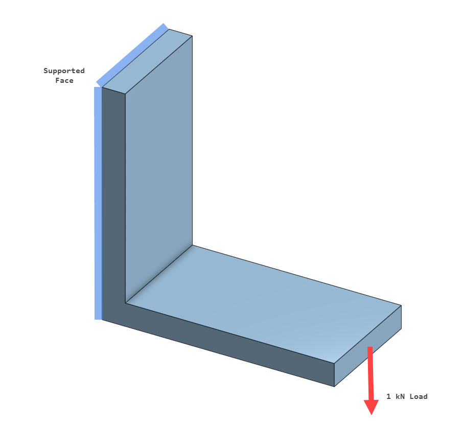
We will consider the case of a bracket under flexural action, as illustrated below:
The project with the geometry, simulation setup and results can be found in the following link:
You can find that we assigned:
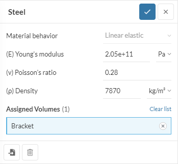
Steel material with default parameters:
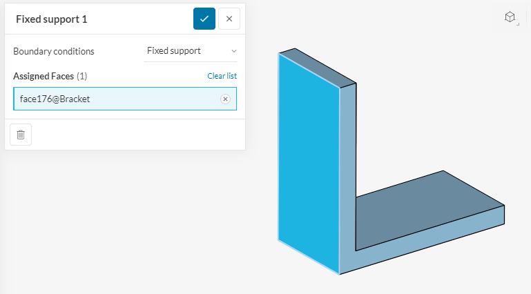
Fixed support condition to the back face:
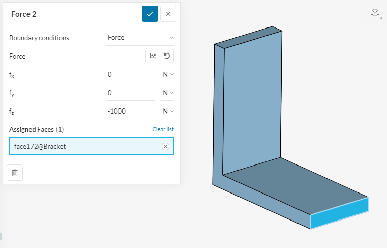
Force condition to the end face:
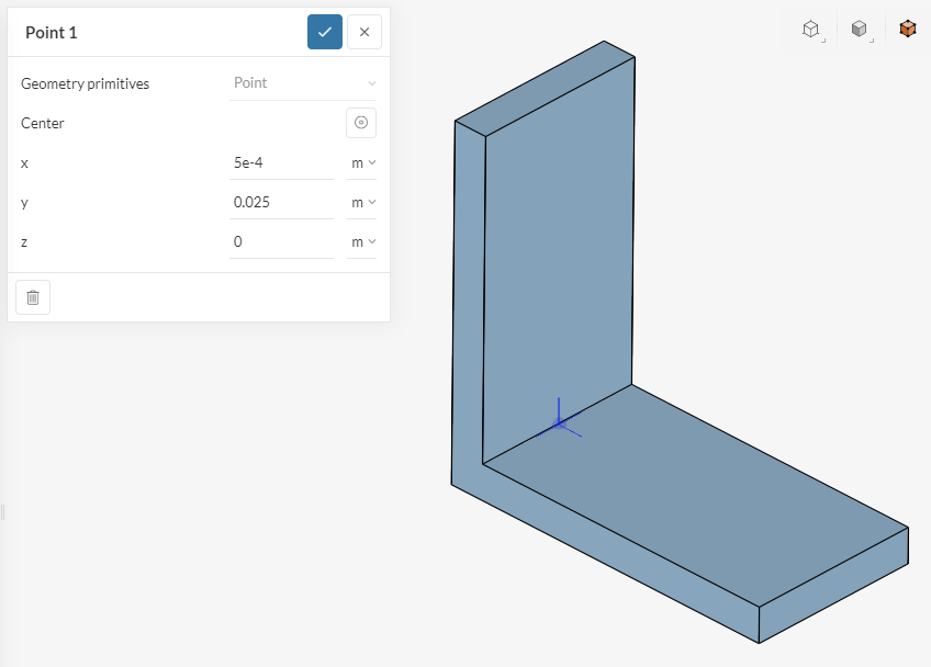
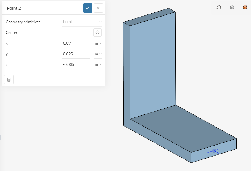
A very important aspect of a convergence study is to compare the results of different meshes at the exact same location. For this, we create a couple of result control items to retrieve the von Mises stress at the root of the corner (Point 1) and the displacement at the end face where the load is applied (Point 2).
Notice that the point at which we measure the stress is not on top of the edge: the reason for this is that, being a stress concentration point, the theoretical stress on the edge is infinite; thus, with mesh refinement the stress value would only increase, converging towards infinity. We pick a point a little to the side of the edge, to get a representative value.
3. Initial Mesh Setup and Results
Our base mesh targets 4 elements across the thickness of the thin walled part, which is a very good starting point (bare minimum would be 2). This is achieved by using manual mesh sizing and SimScale’s Standard meshing algorithm:
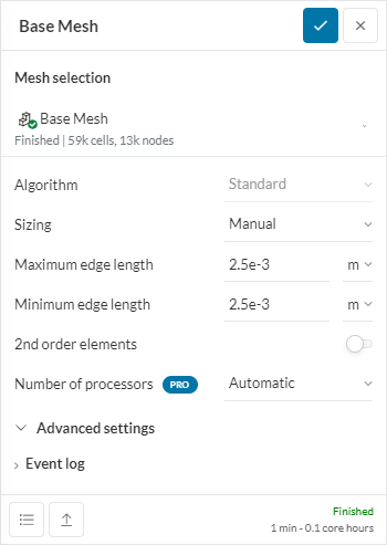
It can be seen that the thickness of the plate is 10 mm, and we specified a mesh sizing (equal maximum and minimum) of 2.5 mm. Here is the result (‘Base Mesh’ in the project):
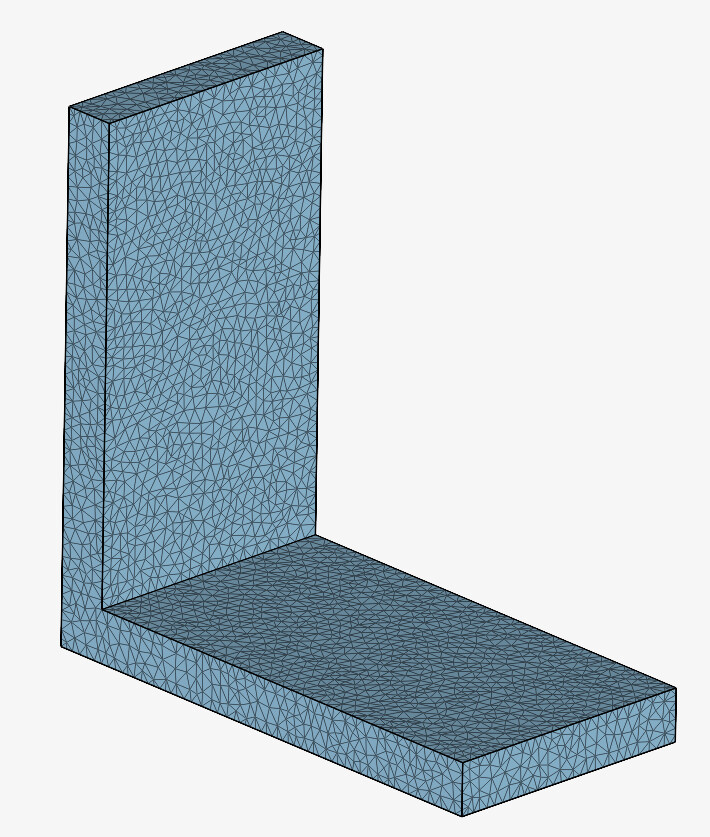
This looks like a very decent mesh (check the Mesh quality if you wish to see the nice Aspect ratios) so we run the simulation (run ‘Base Mesh’) and get the following results for displacement and stress:
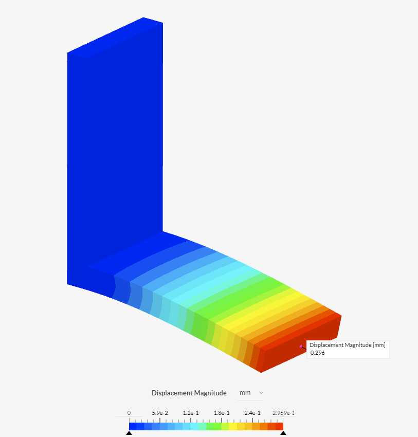

The point data yielded the following results:
- VSM: 83.920 MPa
- DZ: -0.296 mm
We can notice that a gradient of stress is formed at the inner corner, going from red to blue in the color representation in a distance of half a thickness. Also, notice how the gradient is coarsely captured, with jumps and jagged lines contouring the colors. This is how we identify that we need to refine the mesh in this area.
4. Mesh Refinement
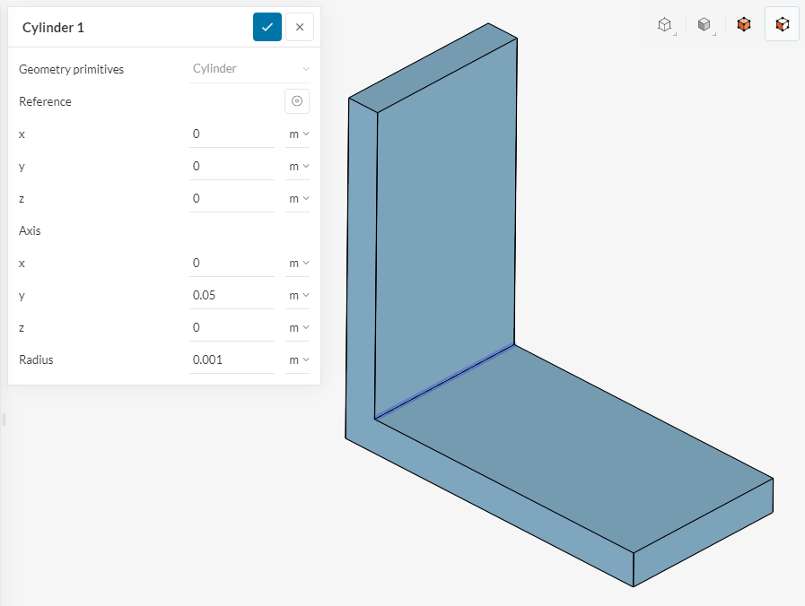
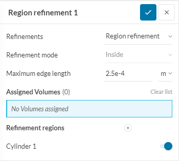
To refine the mesh in the identified region, we use a ‘Mesh refinement’ concept. For this , we create a cylinder that surrounds the inner corner:
As our base mesh length is 2.5 mm, we specify a refinement of 0.25 mm:
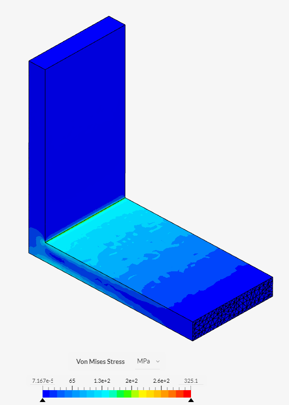
The point data yielded a rather big change in the stress with respect to our base result, and at the same time a small change in the deformation:
- VSM: 147.990 MPa
- DZ: -0.308 mm
If we have a look at the stress contour plot we can see that the gradient is better captured, with the red region being almost unnoticeable:
We repeat this refinement process by decreasing the mesh length on the refinement for until the variation in the results is small enough, in this case only one more iteration was necesary. The process is summarized in the table below:
| MESH | REFINEMENT LENGTH[mm] |
NODES | VMIS [MPA] |
VARIATION % |
DZ [mm] |
VARIATION % |
|---|---|---|---|---|---|---|
| Base Mesh | 2.5 | 13 049 | 83.920 | - | -0.296 | - |
| Refinement 1 | 0.25 | 71 398 | 147.990 | 76.3 % | -0.308 | 4.1 % |
| Refinement 2 | 0.1 | 425 657 | 140.583 | -5.0 % | -0.308 | 0.0 % |
We consider in this case that a variation of 5% is enough to consider the value converged, but in some cases a tighter tolerance can be necessary.
5. Conclusion
A detailed procedure on how to perform a mesh convergence (independence) analysis for FEA simulations using SimScale was showcased, including an example project.
We could find the influence of the mesh on stress and deformation results. Specially, we could see that deformation values converge much faster than stress values near concentration points.
If you are performing a similar study and need some assistance, feel free to post your case!